Article

Methodology and Application of Statistical Techniques to Evaluate the Reliability of Electrical Systems Based on the Use of High Variability Generation Sources

by
César Berna-Escriche
*,
Ángel Pérez-Navarro
,
Alberto Escrivá
,
Elías Hurtado
,
José Luis Muñoz-Cobo
and
María Cristina Moros
Instituto Universitario de Investigación en Ingeniería Energética of the Universitat Politècnica de València (UPV), Camino de Vera s/n, 46022 Valencia, Spain
*
Author to whom correspondence should be addressed.
Sustainability 2021, 13(18), 10098; https://doi.org/10.3390/su131810098
Submission received: 20 July 2021 / Revised: 2 September 2021 / Accepted: 6 September 2021 / Published: 9 September 2021
(This article belongs to the Special Issue Smartgrids and Microgrids Based on Renewable Sources)

Abstract

:
This study presents a new methodology, based on Monte-Carlo techniques to evaluate the reliability of a carbon-free electricity generation system based on renewable sources; it uses as inputs the variation of the electricity demand and the fluctuations in the renewable supply and provides the renewable system to be installed to guarantee a specific supply reliability level. Additionally, looking for a reduction of this renewable system, the methodology determines the improvements by the incorporation of nuclear power and electricity storage. The methodology is of general application, its implementation being possible under different contexts, such as different time horizons and different future energy scenarios, both for developing, emerging, and developed countries. The only requirement is to have a sufficient database from which to make predictions for future scenarios of electrical generation–demand balances. As an example of practical implementation, the electrical system reliability for the particular case of Spain in 2040 has been forecasted. When considering the fluctuations in solar and wind power contributions, very high values of the installed power from these renewable sources are needed to reach a high reliability of the system. These values decrease substantially if contributions from nuclear and storage technologies are included.

1. Introduction

The worldwide demand for primary energy grows continuously [1] and is covered in a high percentage, in the order of 80%, with fossil fuels [2]. This scenario implies a double problem. The first issue is the foreseeable depletion of these types of fuels [3], which would put into question the continuity of the electricity supply in a more or less near future and would have undoubted economic impacts for countries without fossil resources. The second issue, even more serious and in a shorter term, deals with the unacceptable growth of greenhouse gases emissions due to the utilization of these fossil fuels when the need is already to reduce these emissions as much as possible [4,5,6,7].
For several reasons—easiness to be used, necessity to integrate renewable sources in the energy scenario, reduction of end user emissions, etc.—electricity has a growing participation in the final energy consumption of all countries [8], expecting to exceed 30% in the medium term in many of them [9]. Nowadays, electricity generation is based on the use of fossil fuels in more than a 67% and is responsible for about 35% of the total CO2 emissions from the energy sector [2]. Therefore, improving electricity generation up to reach a zero-carbon scenario will reduce dependence on fossil fuels and eliminate GHG emissions in significant percentages, becoming an important element for a sustainable energy system [10,11]. To reach this goal of clean generation, the electricity generation system should be based on renewable sources [12,13]. Nevertheless, due to the lack of reliability of these sources, especially in the case of wind and photovoltaic systems [14,15,16], which are currently the dominant contributors, other non-carbon sources such as nuclear [17,18,19] should be considered. Moreover, the storage of the electricity excess, due to the decoupling between demand and production [20,21,22,23] in the case of renewable sources in the electricity generation, could be added to guarantee a full coverage of the demand at any time.
Due to all the aforementioned considerations, it is necessary to use calculation models to estimate both the demand and the generation of electricity in a zero-carbon scenario with high reliability. In this direction, computer models for energy system planning computer models are not a new tool to estimate long-term electricity system calculations. A huge number of researchers have carried out detailed analyses and reviews in recent years, all of them concentrating on energy system modelling tools [24,25,26,27,28,29,30,31,32,33,34]. In particular, many researchers have developed and used a large number of models; such optimization models can be classified into several groups. There is not a unique model classification, but a widely used classification differences between bottom-up and top-down models, other authors add a category, hybrid models [29,30,31], while others add another additional category, other assessment models [27]. Bottom-up models analyze the system components in detail, i.e., these models focus on the technological complexity of the energy field components. Therefore, bottom-up energy models usually do not take into account the interactions between the energy sector and the other sectors of the economy. Examples of bottom-up models could be MARKAL/TIMES [35,36], ESME [37] or MESSAGE [38] among others. Top-down models consider the energy system as part of a holistic economic system. This means that these models focus on analyzing the interactions between the different sectors of an economy rather than analyzing only energy technologies in depth. Examples of top-down models could be NEMS [39], ENPEP-BALANCE [40] or GEM-E3 [41]. Hybrid models try to overcome the limitations of both types of models by connecting both approaches. Thus, they combine model structures that take into account both technological and macroeconomic aspects. Hybrid model examples could be MARKAL-MACRO [42] and MESSAGE-MACRO [43]. The last group of models, the other assessment models, includes those that cannot be exactly qualified as energy models; in fact, they are macroeconomic models. However, despite being focused on the sustainability of the system in general, they contain an important energy component in their structures. Examples of this last group could be LEAP [44], IMAGE [45] and REMIND [46]. Other authors difference between ESOMs (energy system optimization models) and IAMs (integrated assessment models) families [32]. Both groups of models have many common points, but the main difference is that ESOMs focus on the long-term evolution of energy systems at the level of a group of countries with common links, country, region or even city, while IAMs take into account socio-economic modeling to analyze long-term interdisciplinary issues, usually of global scope. Examples ESOMs could be MARKAL/TIMES [35,36], ESME [37], TEMOA [47] or REMIX [48], while examples of the IAMs could be IMAGE [45], TIAM [49,50], WITCH [51] and REMIND [46].
In line with these forecast models, the current paper presents a new methodology to evaluate the reliability of a carbon-free electricity generation system based on renewable sources and to determine the nominal power to install to cover a specific demand as a function of the demand coverage reliability to be reached. Detailed simulations based on a Monte-Carlo method [52] allow for the determination of the nominal power of the renewable sources to be installed for different reliability levels. The implemented technique takes into account the daily variation of electricity demand profiles and the fluctuations in the renewable source generation, such as wind power and solar photovoltaic. Variations within one day and among days have been considered, both for generation sources and for demand profiles. Additionally, the methodology determines the improvement in reliability by the incorporation of nuclear power and/or electricity storage.
The paper is organized as follows: the current section has introduced the problem and the technical background to address its study; Section 2 details the developed methodology; in the Section 3, this methodology is applied to the case of Spain for the expected electricity scenario in 2040 [53], providing a practical lay out and application of the problem, displaying their results and interpretation; and finally, in Section 4, major conclusions on the methodology and on its application to Spain are detailed.

2. Methodology

To determine the renewable contribution to the electricity generation in a carbon-free situation, we can follow the IEA approach [54]. The total electricity demand is given by:
TED ( t ) = i = 1 5 ED ( i , t )
where ED ( i , t ) is the evolution of the demand from each sector: I = 1 (transport); 2 (industry); 3 (residential); 4 (services), and 5 (agriculture and fishing), being t the specific time considered.
This electricity demand is covered with contributions from the different primary energy sources:
TED ( t ) = j = 1 5 PE ( j , t ) ρ j
where PE ( j , t ) is the evolution of the contribution from each primary energy source: j = 1 (coal); 2 (oil); 3 (natural gas); 4 (nuclear), and 5 (renewable + hydro), and ρ j represents the efficiency, or capacity factor as it is usually referred, of the electricity generation process when using that particular primary energy source.
CO2 emissions from the electricity generation process will be due to the use of the fossil sources in this process. They are given by:
TEM ( t ) = j   = 1 3 PE ( j , t ) e j  
with e j being the specific emissivity, in tons of CO2 emitted for each oil equivalent ton of the primary source j used in the electricity generation process.
The decay of these fossil contributions, in a scenario looking for zero-carbon emissions in the electricity generation, should follow the assumed evolution of the CO2 emissions. So, starting from the values at a particular year t 0 ( t 0 = 2016 in the last available version of the IEA database [55]), we can deduce:
PE ( j , t ) =   PE ( j , t 0 ) · TEM ( t ) TEM ( t 0 )
With the condition to be null for the year t = T f , when the electricity generation should be carbon free, so:
TEM ( T f ) = 0   and   PE ( j , T f ) = 0   for   j   = 1 , 2 , 3
The requirement for renewable energy contribution in that carbon free scenario is given by:
PE ( 5 , T f ) = 1 ρ 5   TED ( T f )
and its evolution to reach the carbon-free situation:
PE ( 5 , t ) = 1 ρ 5 [ TED ( t ) ρ 4 · PE ( 4 , t ) j   = 1 3 ρ j · PE ( j , t ) ]
where PE ( 4 , t ) represents the contribution from nuclear energy to electricity generation that, initially considered as null in T f , could nevertheless be needed to assure a complete reliability of the electricity supply with a lower contribution from renewable sources.
Equations (1) and (6) are usually implemented to deduce the annual requirements in electricity and the total renewable energy contributions for its fulfillment, respectively. Nevertheless, a higher time resolution is needed to deduce the reliability of the electrical system. A 100% reliability requirement for a zero-carbon scenario implies the capability of the installed renewable system to provide the needed energy contributions to fulfill the electricity demand. The use of annual averaged generation values is possible for sources that have low variability or low specific importance in the electricity generation mix, such as: cogeneration, waste, biomass, etc. However, this is not the case for solar photovoltaic and wind energies, whose time dependences are very high [56] and uncorrelated with the electricity demand, while they are responsible for higher contributions to renewable electricity generation [14]. Therefore, to determine the reliability of the electricity supply in a zero-carbon scenario, an energy balance should be made with high time resolution. This total electricity balance (TEB) is given by:
TEB ( t i ) = [ k   = 1 n CF k · PE ( 5 , k , t i ) ] TED ( t i )     0
where CF k · PE ( 5 , k , t i ) is the electricity provided by the k-th renewable generation source at the time t i , and TED ( t i ) is the electricity demand at that time t i .
There are two different ways to consider the contribution of the k-th renewable source, dependent on its time availability. For the case of the above-mentioned fully available sources, their contribution can be estimated as its total electric energy generation capacity PE ( 5 , k , t i ) multiplied by its electric generation efficiency, ρ k . For the variable energy renewable sources, as photovoltaic and wind systems, a more elaborated way to estimate their production must be developed.

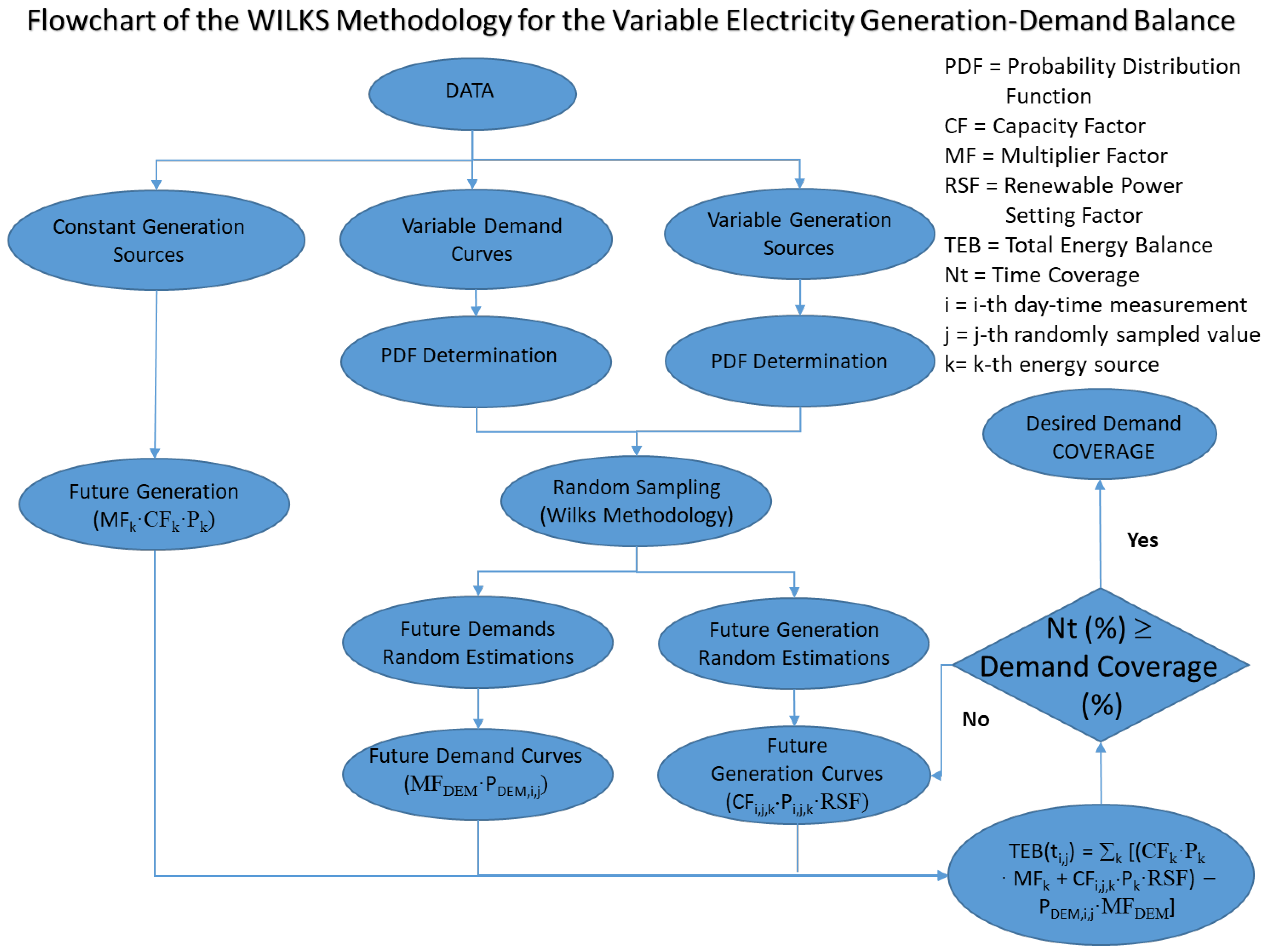
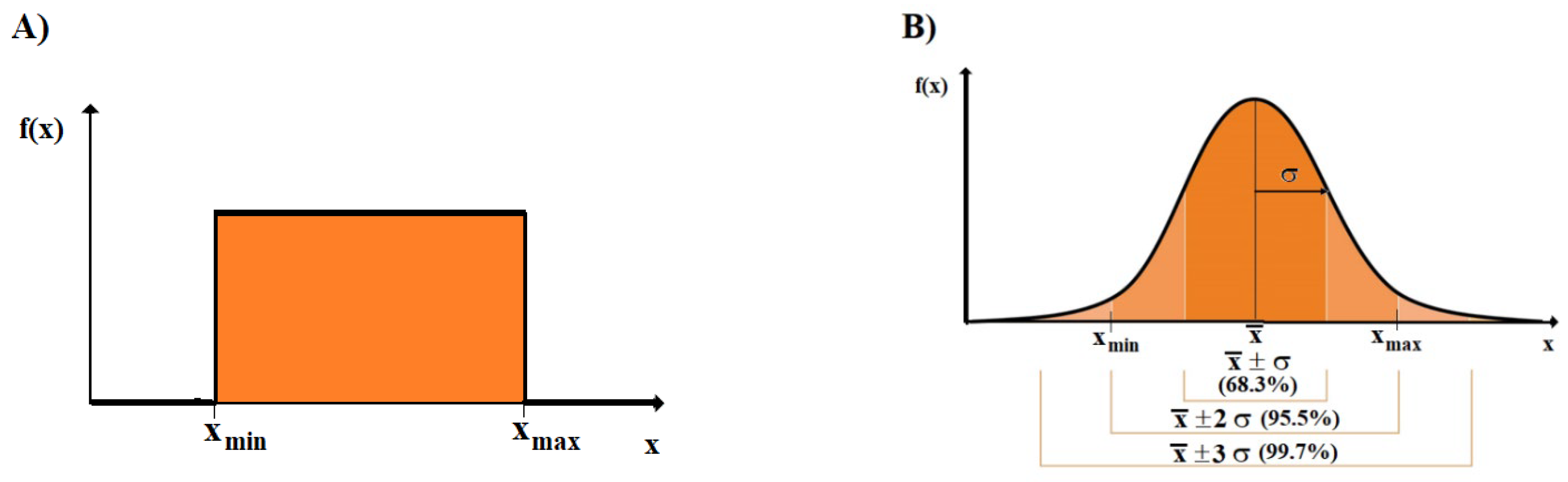
2.1. Statistical Analysis of the Electricity Balance

A possible method for the evaluation of the electricity supply reliability using variable generation sources is the application of a statistical analysis to the existing databases for renewable generation and electricity demand. On this first approach, averaged values are calculated for each one of the time points of the day covered by the database, consequently, the intra-daily variations of these magnitudes along a typical or averaged day are considered.
Using this approach, we can deduce the averaged nominal power of wind and solar photovoltaic sources needed to cover an averaged electricity demand for a particular year in the future. The procedure includes several steps. First, the available historical database for electricity generation and demand should be collected. Second, the extrapolation to a particular time in the future should be addressed. For the electricity demand, daily averaged values deduced from the available database must be obtained and the future demand profile is obtained by applying a multiplier factor to this averaged curve. For the renewable sources, two different groups are considered: low and high variable electricity generation sources. For low variation renewable sources, such as: biomass, hydraulic, cogeneration, residual wastages, etc., the future contributions to electricity generation are obtained by multiplying the calculated mean database values by a multiplier factor. Finally, for the high variable sources, as it is the case for wind and solar PV, an iterative process determines future estimations. The seed value to start the iteration procedure could be the total installed power obtained from a simple electricity balance analysis, which considers a daily equilibrium between electricity generation and demand. Iterations, increasing the renewable power levels, are carried out up to the point in which the electricity balance is positive at all times, reaching, in this case, a 100% supply reliability. Lower reliability values could be accepted if international electricity exchanges to cover electricity shortages are considered.
The expression of the total energy balance at each time measurement point, Equation (8), must be slightly modified to consider the contribution of each renewable source and to estimate demand and generation forecasts:
TEB ( t i ) = k (   CF k · P k · MF k + CF i , k · P k · RSF )   P DEM , i · MF DEM
in which MFk is the multiplying factor of the low variable renewable sources, CFk is a constant capacity factor of each low variability source and CFi,k is a variable capacity factor of each high variability source at each time point, Pk is the currently installed power of each source, RSF is the setting factor of the iterative process for the high variable sources. Finally, the future demand forecast is estimated through the last term of Equation (8), which has been rewritten to consider demand forecast; PDEM,i is the current power demanded at each time; and MFDEM is the multiplier factor for future calculations.
To have the capability to cover the demand, this balance must be zero or positive all the time or during the desired time percentage to reach the degree of demand coverage. Then, defining Nt as the time coverage percentage in which this energy balance is zero or positive:
Nt ( % ) = i Nt i ( TEB   ( t i ) 0 ) i Nt i   · 100
Nti (TEB(ti) ≥ 0) being equal to 1 if TEB (ti) is positive or zero and 0 if negative, ∑ Nti is the total number of measurement points.
Consequently, the iterative process (carried out through the increase of RSF) finishes when Nt(%) reaches 100% reliability or when the desired demand coverage is reached.

2.2. Monte-Carlo Optimization of the Electricity Balance

Nevertheless, the above-described approach does not consider the possible decoupling between electricity demand and variable renewable generation, despite the fact that this effect could seriously compromise the supply reliability. In fact, while the demand profile could be in the high-value zone of its probability distribution function (PDF) for a particular day or period of time, wind and/or photovoltaic production could be in a lower-profile region. Consequently, in this hypothetical situation, the demand would be far from being met, although on average it would be fully covered. Therefore, a more detailed analysis taking into account these possibilities led to the development a stochastic approach that could be addressed by using a Monte-Carlo simulation method. Then, under these conditions, not only intra-daily variations have to be considered, but also the inter-daily ones, in such a way that all variables are randomly sampled covering the whole range of values in their PDF. The Wilks methodology has been followed [57,58] for the Monte-Carlo analysis in this study.
Figure 1 displays a flowchart of the methodology followed to carry out this Monte-Carlo analysis. The major difference with the statistical approach resides in the use of a random sampling for the variables following a PDF with a high daily variability, i.e., electricity demand, solar photovoltaic and wind generation. In particular, 59 random combinations of values for these three variables were used. This choice is justified because the output variable under study, the electricity generation–demand balance, has only a one-side interval restriction to meet (electric balance has to be zero or positive, not comprised between two values) and the coverage and confidence intervals obtained with this number of combinations allows for a 95 × 95% confidence and coverage percentages [57,58]. The multi-variable analysis approach of the Wilks formula obtained by Wald [59,60] could also have being used with the same number of random combinations, as this methodology needs the same number of random simulations than Wilk’s for one-side interval output variable.
In this Monte-Carlo approach, an important factor is the estimation of the PDF followed by each variable. Then, the application of the methodology begins with the estimation from the historical database of the PDF followed by each variable. To determine the PDF followed by the different variables, several goodness-of-fit tests have been performed for the data; in particular, the Kolmogorov–Smirnov test has been used to estimate the best fit PDF. In the case that normal is the best-fit PDF, complementary tests such as Chi-square, Shapiro–Wilk statistic and Z-value for both skewness and kurtosis have been performed to reaffirm that the distribution of this variable is compatible with the normal distribution. Uniform and normal are considered to be the most common PDFs found for the different variables. In the case of a uniform PDF, only the minimum (xmin) and maximum (xmax) values allowed to the variable have to be determined (Figure 2A). For a normal PDF, the mean and variance have to be determined, but also the desired coverage, which usually is 95%, then the minimum and maximum values are determined as displayed in Figure 2B.
Random sampling of Wilks’ methodology consists of 59 random combinations of groups of values for all variables involved in the electric energy balance at all database measurement points. Since all databases have a temporary resolution (number of daily measurement points, Figure 3A), a random sampling should theoretically be carried out for each one of these points. Each sampling should independently follow the variable PDF at each measurement point (Figure 3B displays a variable following different Gaussian PDFs for each time data point). However, an “independent random sampling” for each daily measurement point (Figure 3C) is not an appropriate estimation because there could be a very large variation between sampled values of two adjacent points of a variable. In the extreme case, it would be possible to change from maximum to minimum values of a variable between two adjacent measurement points, having the variable a very pronounced saw-tooth shape (Figure 3D), a condition that would be almost impossible to happen in reality.
Consequently, instead of this unrealistic situation, what has been carried out is a “single random sampling”, i.e., only one sampling consisting of 59 random combinations of values for all the considered variables (Figure 4). However, by proceeding in this way, one database point has to be chosen, for instance, the one with a greater dispersion among all the daily resolution points, the point for which the random sampling is carried out (Figure 4A), after which the extrapolation of the 59 sampled values has to be carried out to the remaining time points. For each sampled point, the upper and lower tails are estimated (Figure 4B). In all cases, the allocation of the upper and lower tails of the PDF would be maintained among all the daily temporary database resolution (Figure 4C), i.e., it could be said that the whole averaged curve of each variable is shifted to include the sampled point but considering the PDF followed by each point (Figure 4D).
The way in which each random value would be extrapolated to each time data point depends on the PDF followed by each variable: in most cases, normal or uniform PDFs. For a uniform PDF, given a sampling value, as the interval limits are known, it is easy to extrapolate for the remaining data time points; it is only needed to keep constant the relative tail length (percentage of values above and below the sampled value). For the case of a normal PDF, given a sampling value, the parameters characterizing the normal PDF (mean and standard deviation) are known. Therefore, the allocation of its upper and lower tails can be maintained constant for the remaining time points. For this, the simplest way will be the conversion of the normal followed by each variable at the selected temporal data point to the standard normal, i.e., for the selected point, the transformation Y = X μ σ will be applied, so that Y will follow an N(0,1). Then, this value will be kept constant for all time data points. Therefore, finally, by undoing this transformation, the values of the remaining points with the particular values of their PDF and keeping the same lower-upper tails as the initial point will be obtained. In summary, the curves followed for each of the 59 shortlists of sampled values are estimated; the averaged curves are shifted to include the sampled points. As a result, the electricity balance can be calculated for each group of curves.
From this point, the procedure is similar to the one described in the previous section, with the only difference being that the total energy balance is extended to the 59 sets of randomly sampled variable values of the Wilk’s methodology. The 59 electric energy balances are carried out, the balance of balances, has to cover the demand at the desired degree (for instance, at a 99% or all the time). The total energy balance for each time measurement point and for each sampled value is:
TEB ( t i , j ) = k (   CF k · P k · MF k + CF i , j , k · P k · RSF )   P DEM , i , j · MF DEM
in which CFi,j,k is the capacity factor of each high variability source at each time point for each sampled value and PDEM,i,j is the current power demanded at each time and for each sampled value.
In order to cover the demand, this balance has to be higher or equal to zero during all the time or during the desired time percentage. Then, defining Nt as the time percentage in which this energy balance is positive:
Nt ( % ) = i , j Nt i , j ( TEB   ( t i , j ) 0 ) i , j Nt i , j · 100
As for the statistical analysis, the iterative process (carried out through the increase in RSF) also finishes when Nt(%) reaches 100% demand coverage or when the desired reliability is reached. To start the iteration procedure, the same seed values than in the previous case would be used; of course, in this first step, the averaged generation–demand balance only covers a percentage of the demand. Then, as explained in the previous method, an iterative process is carried out to improve this balance—a process that finishes when a positive final electric generation–demand balance is achieved for every time interval, or when a lower electric energy coverage percentage is reached, considering that international exchanges could cover the time period in which demand is not fully covered.
In order to reduce the requirements on renewable sources, the methodology also considers the possibility to include in the electricity generation scenario other non-carbon sources, as is the case for nuclear energy and, given the decoupling between generation and demand, also the possibility of electricity storage in order to reduce the amount of electricity excess.

3. Results and Discussion

In this section, the development of the methodology applied to a particular case is carried out. Specifically, the definition and approach of the problem is presented, together with the necessary information to arrive at the most accurate predictions possible, so that, finally, the results obtained are exposed and their subsequent discussion. In particular, the application of the previously developed methodology to the specific case of Spain has been carried out, aiming to estimate the needed renewable power to install in order to reach a full reliability electricity supply in a zero-carbon scenario.
Although the methodology has been applied to forecast the particular case of Spain in 2040, this methodology is of general application. So, it is possible to implement the described method under different contexts, such as different detail degrees of the available information, of time horizons and of future energy scenarios, both for developing, emerging, and developed countries. The only requirement is to have a sufficient database from which to make predictions for future scenarios of electrical generation–demand balances, in such a way that the carried-out calculations have a sufficiently solid starting point, and consequently, the reached conclusions are consistent enough too.
Concentrating on the example of the methodology application, apart from the economic crisis period (2008–2013), there has been a continuous increase in the electricity demand in Spain, mainly from the industrial, residential, and service sectors, as can be deduced from Figure 5 obtained using the IEA database [55]. Figure 6 shows the data for total electricity demand and the fraction that electricity represents in the total consumption of final energy and their lineal extrapolation up to the year 2040. The obtained results indicate an increase in the contribution of electricity up to 32% with a demand of electricity of about 30 Mtoe (3.49⋅102 TWh), a factor 3 over the values in 1990.
Contributions from each primary energy source to electricity generation [55] are shown in Figure 7. Using the specific emissivity of the fossil fuel detailed at Table 1, and the amount of each fossil fuel contribution to electricity generation, we can deduce the CO2 emissions in this generation process. Total emissions and its exponential extrapolation up to zero carbon emissions in 2040 are plotted at Figure 8.
Using Equation (4), we can calculate the amount of each fossil fuel contribution and its evolution up to be null in 2040. The results are plotted in Figure 9; applying Equation (7), the required amount of renewable energy is deduced and displayed in Figure 10. The contribution of primary energy sources to the electricity generation are calculated assuming a nuclear shutdown of all the nuclear plants in Spain for the year 2025.
Assuming the values in Table 2 for the generation efficiency and the number of annual operation hours at the nominal power of the different generation systems, we can deduce the required nominal power of these systems for the evolution of the generation process up to reach zero carbon emissions in 2040 (Figure 11).
The values displayed at Figure 11 are only a first approach to the needed nominal power of the renewable electricity generation system, because only mean annual values of the energy generation sources are used (only averaged capacity factor for several generation sources are considered). To determine a more realistic estimation of that power, the methodologies described in the previous section are applied. In this section, the application of the previously developed methodology to the case of Spain, looking for a zero-emission scenario in the year 2040, is carried out. REE data for February 2017 have been used and three different distributions between wind and solar photovoltaic contributions to the total installed renewable power are considered: 40–60%, 50–50% and 60–40%, respectively.

3.1. Statistical Approach

Using the REE data [61], the PDF followed by each variable has been obtained and, using them, the two analyzed models based on a statistical approach have been addressed. The first of them only uses the PDFs averaged values, while in the second model, using the Monte-Carlo Wilks methodology, PDF averaged values and their standard deviations are used.

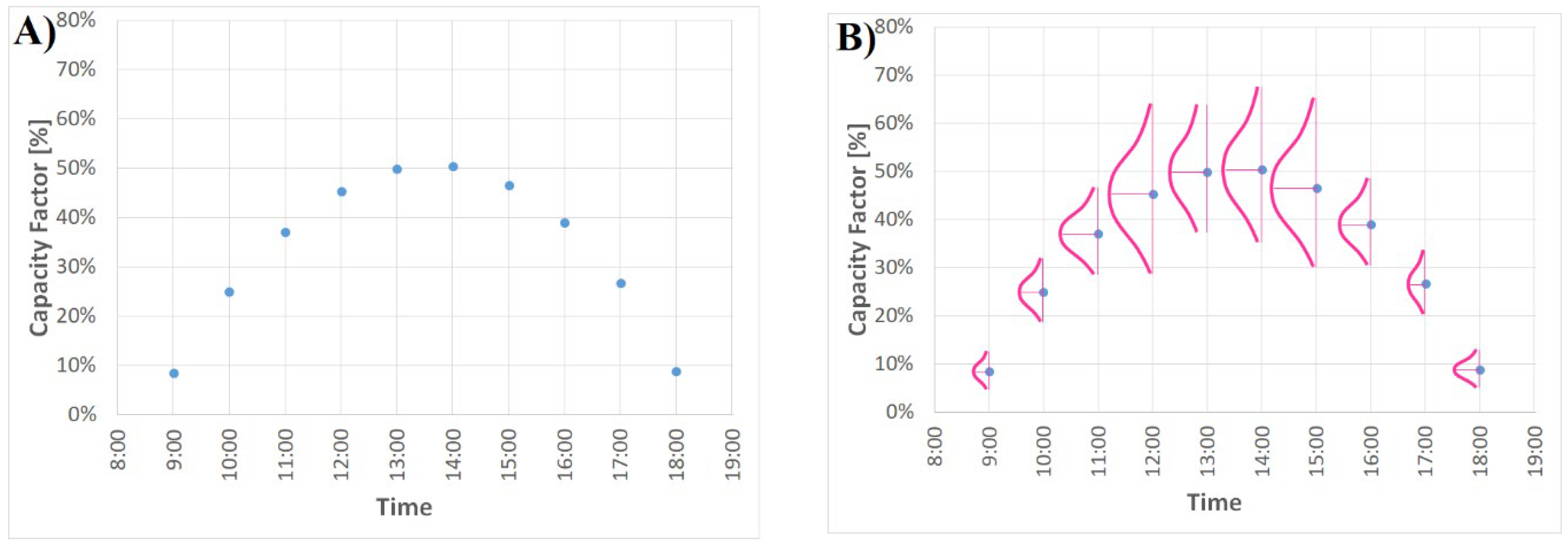
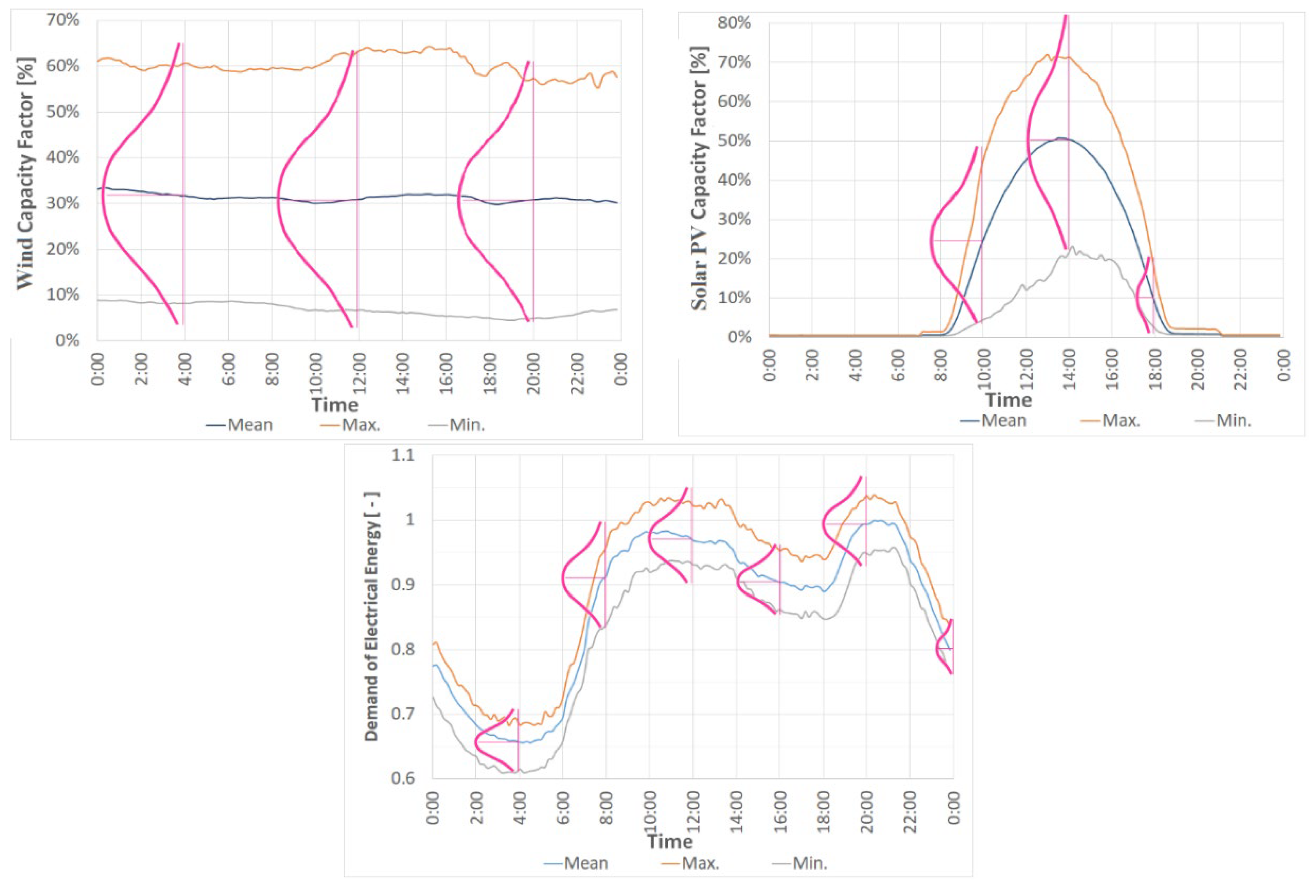
3.1.1. Data Analysis

REE data for each variable with daily variation (demand, wind and solar photovoltaic) has been analyzed and their PDFs have been calculated. As the REE data have a resolution time of 10 minutes, then 144 time data points per variable and day are available. Consequently, 144 different PDFs per variable can be obtained. All of them have turned out to be normal distributions, whose mean and standard deviation values are summarized in Table 3. Figure 12 displays the mean, maximum and minimum values along the day and, superimposed, several PDFs for specific time values. Along the complete study, we are assuming that these PDFs maintain the same structure up to 2040.
For the other variables (which include the rest of renewable energies, such as hydraulic, cogeneration or residual wastages), their estimations have been carried out by using the mean values of the current generation and the assumption of a multiplying factor to consider future increases in 2040. Table 4 details the characteristics of the renewable sources and the assumed values in 2040.

3.1.2. Daily Averaged Approach

Considering the intra-daily variations in the electricity generation and demand, the procedure described in Section 2.1 has been performed. The obtained results, after the iterative process, are shown in Figure 13. The total renewable power needed to cover the demand with a reliability of 99% for the three considered renewable distribution between wind and photovoltaic sources are 191.1, 222.4 and 268.6 GW, respectively.

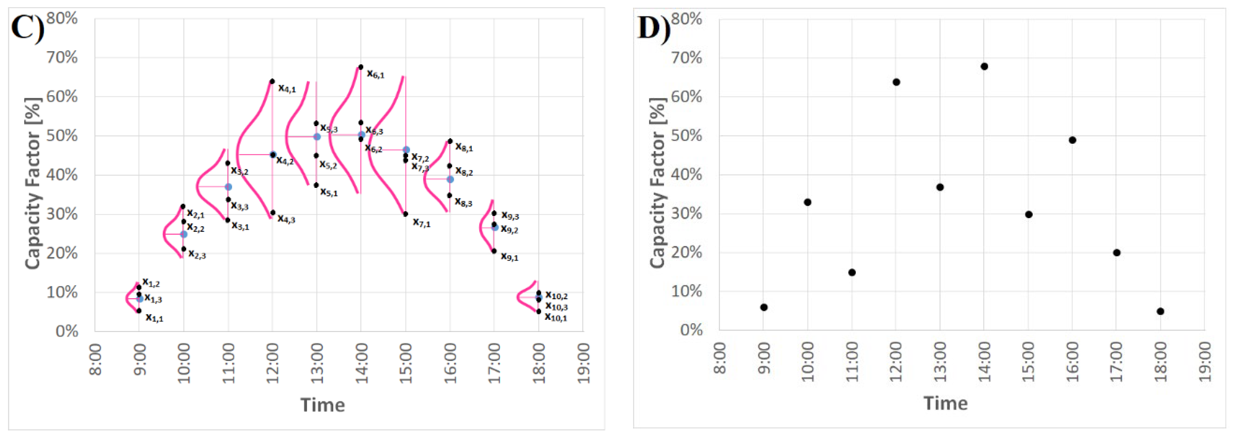
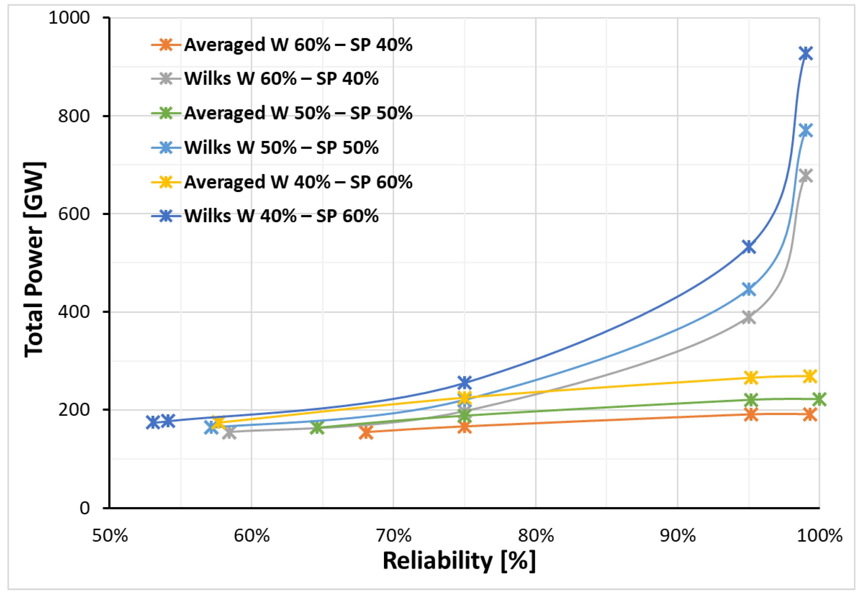
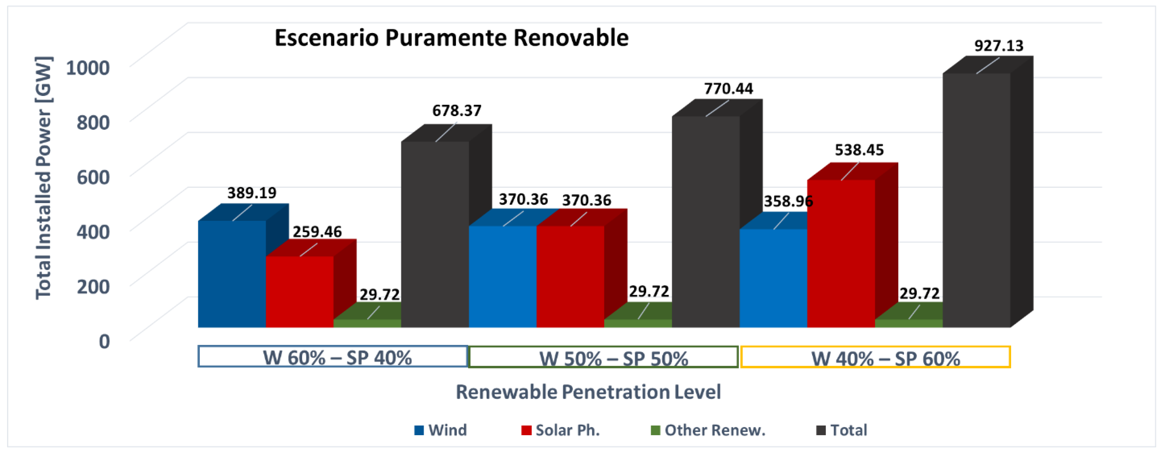
3.1.3. Monte-Carlo Approach

Using Monte-Carlo techniques, in particular, the Wilks’ approach, the procedure described in Section 2.2 is carried out. As in the previous approach, an additional study has been carried out for the three possible scenarios of wind and solar photovoltaic distribution levels. Final electricity balances are shown in Figure 14 for the three scenarios.
The results of the two statistical analysis models for different demand coverage are displayed in Figure 15. Significant increases in the needed power are obtained when the most accurate approach, the Monte-Carlo method, is used. As shown in Table 5 and Figure 15 and Figure 16, total installed powers between 700 and 900 GW are needed to cover the electric demand for all the three renewable penetration level scenarios. In the case under study, the differences in the total installed power between the consideration of an averaged day and the Monte-Carlo analysis to carry out the calculations led to a factor higher than 3 in the power requirements for reliabilities approaching 100% of the time demand coverage.

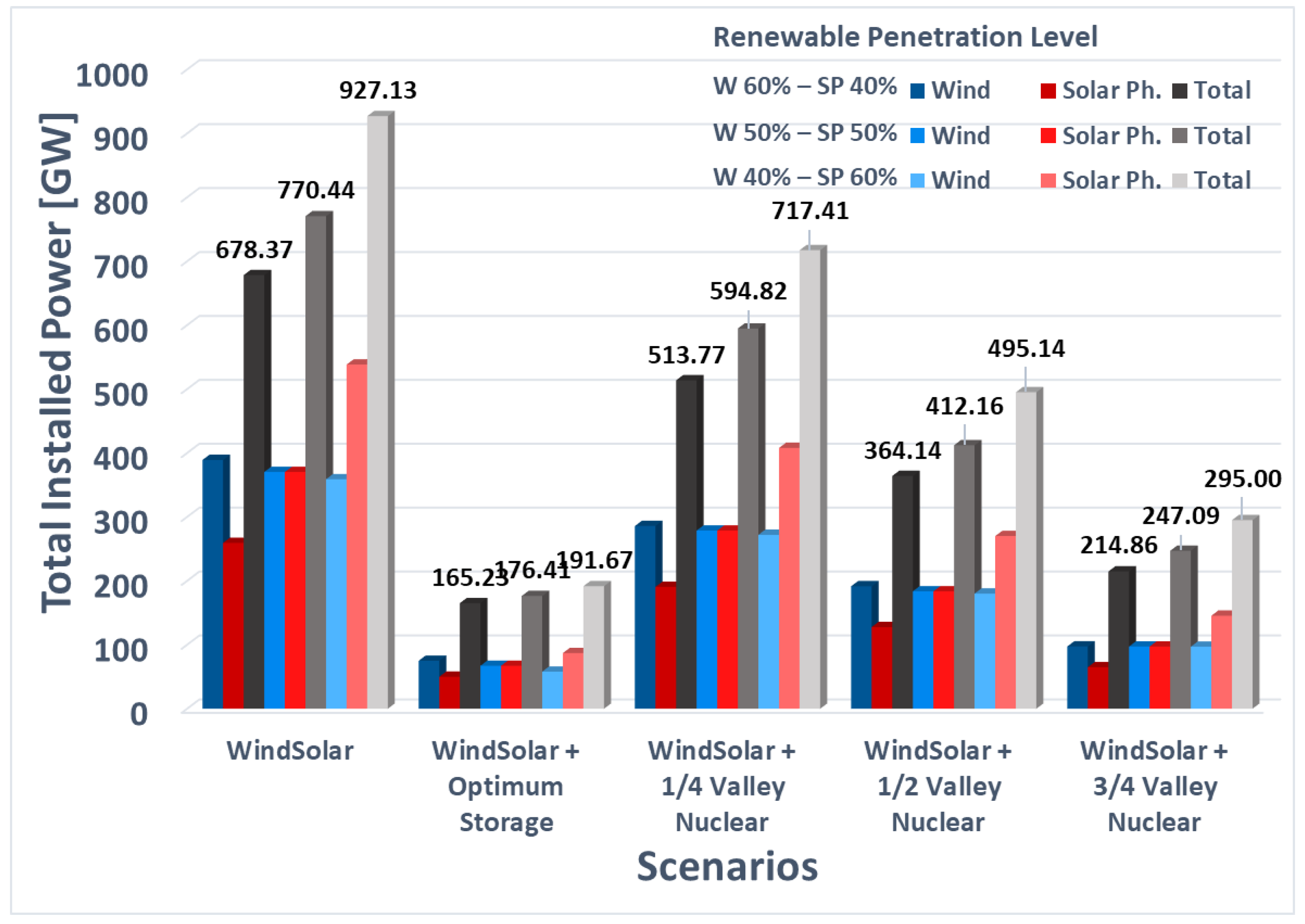
3.2. Additional Strategies Based on Nuclear Energy and Electricity Storage

Considering that the electricity demand prediction for Spain in 2040 is about 3.49⋅102 TWh, as shown at Figure 6, a total installed power of 40 GW to cover this demand would be required, assuming a constant demand curve over time. Consequently, using only renewable energies, the Monte-Carlo results indicate the need for an increase in the order of a factor of 20 over this initial value. Then, in order to make a future renewable scenario with zero CO2 emissions in the electricity generation possible, the renewable energies should be supported by other non-polluting generation options. One possible strategy is the use of nuclear energy, which is being used in Spain at this moment. With a total installed power of 7.6 GWs and a capacity factor of 93.4% (data of REE for 2017 [61]), it has a value that is approximately a quarter of the valley demand estimated for the year 2040. The second strategy could be the storage of the electricity generation excess; currently there is in Spain a total power installed of 5 GW, mostly as pumping storage power plants. The pumping storage is not the only way to take advantage of the excess of electricity generation. The use of mega-batteries could be another possible way in the near future, or the use as distributed storage of the large fleet of electric vehicles, which is also expected in the near future, or even other storage technologies that can appear or become worthwhile in the considered 20 year time horizon.
Summarized results of the analyzed scenarios using Monte-Carlo’s approach and including nuclear power and electricity storage are displayed in Figure 17, Figure 18 and Figure 19. This Monte-Carlo approach is the most accurate, since it takes into account the variations for both generation and demand along time, considering their fluctuations between days and within a day. In these three figures, the pure renewable scenario has been also displayed in order to have a reference value. Results for renewable generation, plus the current nuclear installed power and its double and triple values, which approximately coincide with a quarter, half, and three quarters of the valley demand previsions for 2040, are displayed in Figure 17. Similarly, the renewable generation plus current, double, and quadruple of the installed storage capacity are displayed in Figure 18. Finally, Figure 19 shows the combined use of nuclear and storage strategies to reduce renewable power requirements to be installed.
The maintenance of Spain nuclear power, 7.6 GW, shows an important reduction of about 200 GW of the total installed renewable power needed to cover the growing demand. By doubling or tripling this nuclear power, significant additional reductions would be reached, as shown in Figure 17.
Another possible strategy would be the development of storage technologies, as shown in Figure 18. During the whole storage process, an efficiency of 80% has been considered for all possible storage technologies (20% losses during pumping-turbine processes in pumping stations, loading–storage–discharge in battery storage, or in any other storage technology). The existing 5 GW of storage power capacity would lead to significant reductions in renewable power needed to cover the demand. Reductions from about 925 to 250 GW would be reached. The amounts would have additional reductions, to about 175 GW, if the storage power capacity was increased up to 20 GW.
The combined use of renewable energies supported by both technologies—nuclear generation and storage technologies—would lead to even better achievements, as displayed in Figure 19. The renewable power to install reaches values of approximately 180 GW for the current nuclear power and storage capacity. Achieving even higher reductions, up to approximately 100 GW of total installed power, when increasing the nuclear installed power by a factor of 3 and the storage capacity by a factor of 4.
The influence in the total installed power when considering the different nuclear generation and storage powers capacities is summarized in Figure 20. As mentioned above, the use of storage technologies is necessary when having important contributions of variable renewables energies, because unacceptable values of installed power are required. Reductions from about 700 or 900 GW, depending on the renewable penetration scenario, to approximately 200 GW with only a few GWs of storage capacity. Even higher reductions, when maintaining or increasing the currently installed nuclear power, are achieved at approximately a rate of 5 GW of total power needed per installed GW of nuclear generation power.

3.3. Dependency between Scenarios and Energy Wastages

Another drawback of the pure renewable scenario, which has not been mentioned up to this moment, is the enormous amount of energy wasted (Table 6 and Figure 21, Figure 22 and Figure 23). The three pure renewable levels indicate that, using only renewable energies to cover the demand, a huge amount of energy per day is lost; the unused energy is mainly concentrated in the central day hours, in which the generation exceeds the demand, fundamentally due to the solar photovoltaic contribution (Figure 13, Figure 14, Figure 15 and Figure 16). The wasted electric energy for the pure renewable scenario is between 3.2 and 3.9 TWh depending on the renewable component scenario. The highest value belongs to the W 40% – SP 60% renewable penetration scenario, while the lowest corresponds to the W 60% –SP 40%. These values could be significantly reduced, simply by maintaining the installed nuclear generation power, by approximately a factor of 2. Meanwhile, the current storage capacity reduces the wasted energy by about a factor of 4. All these values would have additional reductions if the current capacities of both technologies would be increased, reaching a factor of about 30 when tripling the current nuclear power and quadrupling the current storage capacity.

4. Conclusions

Throughout the last decades, and even today, in most countries, the growing worldwide energy demand has been and is mainly covered with fossil fuels. This is a scenario that fundamentally lays out a double problem: the unavoidable depletion of fossil fuel reserves and, even more relevant, an unacceptable growth of greenhouse gases emissions. Focusing on electricity, this source has a growing participation in the final energy consumption; consequently, achieving zero emissions in electricity generation is a must for a sustainable energy system. This study has developed a methodology capable of evaluating the reliability of any possible scenario, particularly a carbon-free electricity generation system based on renewable sources. A methodology, which is in turn based on Monte-Carlo sampling, has been presented; in particular, the Wilks methodology has been used to simulate different scenarios for electricity generation and evaluate their reliability to cover the electricity demand. The intra and inter daily variation of electricity demand profiles and these fluctuations in the renewable sources, particularly wind and solar photovoltaic, have been considered. Finally, using all these considerations, the nominal renewable power to be installed in order to cover the demand can be estimated.
As an example of practical application, the developed methodology has been applied to forecast the electricity generation–demand balance in Spain for the year 2040, extrapolating the data from February 2017. The implementation of a pure renewable scenario would lead to unacceptable values of the total power to be installed, depending on the distribution of the wind and solar photovoltaic generation, in the assumed scenario between approximately 700 GW and more than 900 GW. These are huge values considering that the yearly averaged forecasted demand is about 40 GW with peaks of approximately 50–55 GW. Evidently, this enormous amount of renewable power needed to cover the demand with full reliability is not a realistic quantity to install and, additionally, this installed power would lead to a massive amount of wasted energy in many day periods. In particular, this shortcoming would be accentuated during some of the central day hours, specifically when solar photovoltaic would be at its production peak and demand would not be close to its maximum value. Consequently, other generation technologies must be explored. One suitable approach would be the use of nuclear energy and storage technologies in combination with renewable generation. This solution reduces significantly the required renewable power. In particular, maintaining the currently installed power of nuclear energy in Spain, the renewable power to be installed is reduced in about 200 GW. The total power is reduced to about 200–250 GW, depending on the renewable penetration distribution, if the current installed storage capacity is maintained. The joint use of both technologies—nuclear and storage—would lead to about 150 GW, with the currently existent power capacities. The quantity that would reach less than 100 GW with 22GW of nuclear power installed and the currently installed storage capacity would be 5 GW. In addition, the vast amount of energy lost would reduce drastically, from around 3–4 TWh of the pure renewable scenario to close to 0.1–0.2 TWh with the upgraded nuclear and storage capacities.
In conclusion, two remarks can be drawn from the application of the methodology to foresee the electricity balance in Spain for the year 2040, remarks that could also be applied to a greater or lesser extent to any other country. The strong commitment to implement a purely renewable electric energy generation mix would lead to two major drawbacks. The first is the need to install unaffordable power values to cover the electric demand. The second is the enormous energy wastages. Consequently, alternative generation sources meeting the conditions of zero CO2 emissions have to be added. An appropriate approach would be the use of nuclear generation energy and storage technologies in combination with renewable generation. This solution, maintaining the condition of zero carbon emissions, would significantly reduce the renewable power to be installed and, at the same time, the energy wastage would also be significantly reduced.
Finally, it should be emphasized that the application of the developed methodology is only an example. Although the predictions will probably be acceptably good, to predict any future annual balance, and consequently to determine the power to be installed to cover it, not only one month should be analyzed. Instead, at least the data from a typical winter month and a summer month, and probably even a typical autumn and spring month should be analyzed as well. Ultimately, for a better forecast, it probably would be convenient to analyze the data for each month of a year, so that the power to be installed would be the maximum of these minimum powers required to cover the demand in any of them. To conclude, it is possible to implement the described Monte-Carlo methodology under different contexts, such as developing, emerging, and developed countries, for different detail degrees of the available information, time horizons and/or future energy scenarios. The only requirement is to have a sufficient database from which to make predictions for future scenarios of electrical generation–demand balances. Otherwise, the corresponding assumptions must be assumed, with the risk of arriving at not so accurate predictions.

Author Contributions

Conceptualization, Á.P.-N. and C.B.-E.; methodology, C.B.-E. and J.L.M.-C.; software, A.E. and C.B.-E.; validation, Á.P.-N., J.L.M.-C., E.H. and M.C.M.; formal analysis, E.H. and M.C.M.; investigation, C.B.-E., A.E. and E.H.; resources, A.E. and Á.P.-N.; data: A.E. and C.B.-E.; writing—original draft preparation, Á.P.-N. and C.B.-E.; writing—review and editing, A.E., E.H. and M.C.M.; results interpretation, all authors. All authors have read and agreed to the published version of the manuscript.

Funding

This research received no external funding.

Institutional Review Board Statement

Not applicable.

Informed Consent Statement

Not applicable.

Conflicts of Interest

The authors declare no conflict of interest.

References

  1. International Energy Agency, 2018. World Energy Outlook 2018. Summary Executive. Available online: https://webstore.iea.org/download/summary/190?fileName=English-WEO-2018-ES.pdf (accessed on 11 February 2019).
  2. British Petroleum, 2019. BP Energy Outlook 2019. British Petroleum. Available online: https://www.bp.com/content/dam/bp/business-sites/en/global/corporate/pdfs/energy-economics/energy-outlook/bp-energy-outlook-2019.pdf (accessed on 3 February 2021).
  3. Whiting, K.; Carmona, L.G.; Sousa, T. A review of the use of exergy to evaluate the sustainability of fossil fuels and non-fuel mineral depletion. Renew. Sust. Energ. Rev 2017, 76, 202–211. [Google Scholar] [CrossRef]
  4. IPCC. Renewable Energy Sources and Climate Change Mitigation: Special Report of the Intergovernmental Panel on Climate Change; Cambridge University Press: Cambridge, UK, 2012; ISBN 978-1-107-60710-1. [Google Scholar]
  5. PBL Netherlands Environmental Assessment Agency. 2017. Growth in Global Greenhouse Gas Emissions Resumed in 2017. Available online: https://www.pbl.nl/en/news/newsitems/2018/growth-in-global-greenhouse-gas-emissions-resumed-in-2017 (accessed on 28 January 2021).
  6. Jiang, X.; Guan, D. Determinants of global CO2 emissions growth. Appl. Energy 2016, 184, 1132–1141. [Google Scholar] [CrossRef] [Green Version]
  7. Henriques, S.T.; Borowiecki, K.J. The drivers of long-run CO2 emissions in Europe, North America and Japan since 1800. Energy Policy 2017, 101, 537–549. [Google Scholar] [CrossRef]
  8. Zhao, W.; Cao, Y.; Miao, B.; Wang, K.; Wei, Y.-M. Impacts of shifting China’s final energy consumption to electricity on CO2 emission reduction. Energy Econ. 2018, 71, 359–369. [Google Scholar] [CrossRef]
  9. European Commission. Strategic Energy Technology (SET) Plan; European Commission: Luxembourg, 2017; ISBN 978-92-79-74277-4. [Google Scholar]
  10. Zaman, K.; Moemen, M.A. Energy consumption, carbon dioxide emissions and economic development: Evaluating alternative and plausible environmental hypothesis for sustainable growth. Renew. Sust. Energ. Rev. 2017, 74, 1119–1130. [Google Scholar] [CrossRef]
  11. Sun, X.; Zhang, B.; Tang, X.; McLellan, B.C.; Höök, M. Sustainable energy transitions in China: Renewable options and impacts on the electricity system. Energies 2016, 9, 980. [Google Scholar] [CrossRef] [Green Version]
  12. De Llano Paz, F.; Calvo-Silvosa, A.; Iglesias Antelo, S.; Soares, I. The European low-carbon mix for 2030: The role of renewable energy sources in an environmentally and socially efficient approach. Renew. Sust. Energ. Rev. 2015, 48, 49–61. [Google Scholar] [CrossRef]
  13. Cirstea, S.; Cirstea, A.; Steluta Martis, C.; Fülöp, T.M. Current situation and future perspectives of the romanian renewable energy. Energies 2018, 11, 3289. [Google Scholar] [CrossRef] [Green Version]
  14. Huber, M.; Dimkova, D.; Hamacher, T. Integration of wind and solar power in Europe: Assessment of flexibility requirements. Energy 2014, 69, 236–246. [Google Scholar] [CrossRef] [Green Version]
  15. Belderbos, A.; Delarue, E. Accounting for flexibility in power system planning with renewables. Int. J. Electr. Power Energy Syst. 2015, 71, 33–41. [Google Scholar] [CrossRef] [Green Version]
  16. Ndawula, M.B.; Djokic, S.Z.; Hernando-Gil, I. Reliability enhancement in power networks under uncertainty from distributed energy resources. Energies 2019, 12, 531. [Google Scholar] [CrossRef] [Green Version]
  17. Hong, S.; Bradshaw, C.J.A.; Brook, B.W. Global zero-carbon energy pathways using viable mixes of nuclear and renewables. Appl. Energy 2015, 143, 451–459. [Google Scholar] [CrossRef]
  18. Cany, C.; Mansilla, C.; Mathonnière, G.; da Costa, P. Nuclear contribution to the penetration of variable renewable energy sources in a French decarbonized power mix. Energy 2018, 150, 544–555. [Google Scholar] [CrossRef]
  19. Suman, S. Hybrid nuclear-renewable energy systems: A review. J. Clean. Prod. 2018, 181, 166–177. [Google Scholar] [CrossRef]
  20. Mohamad, F.; Teh, J.; Lai, C.-M.; Chen, L.-R. Development of energy storage systems for power network reliability: A review. Energies 2018, 11, 2278. [Google Scholar] [CrossRef] [Green Version]
  21. Lazkano, I.; Nφstbakken, L.; Pelli, M. From fossil fuels to renewables: The role of electricity storage. Eur. Econ. Rev. 2017, 99, 113–129. [Google Scholar] [CrossRef] [Green Version]
  22. McPherson, M.; Johnson, N.; Strubegger, M. The role of electricity storage and hydrogen technologies in enabling global low-carbon energy transitions. Appl. Energy 2018, 216, 649–661. [Google Scholar] [CrossRef]
  23. Kharel, S.; Shabani, B. Hydrogen as a long-term large-scale energy storage solution to support renewables. Energies 2018, 11, 2825. [Google Scholar] [CrossRef] [Green Version]
  24. Bhattacharyya, S.C.; Timilsina, G.R. A review of energy system models. Int. J. Energy Sect. Manag. 2010, 4, 494–518. [Google Scholar] [CrossRef]
  25. Amorim, F.; Pina, A.; Gerbelová, H.; da Silva Pereira, P.; Vasconcelos, J.; Martins, V. Electricity decarbonisation pathways for 2050 in Portugal: A TIMES (The Integrated MARKAL-EFOM System) based approach in closed versus open systems modelling. Energy 2014, 69, 104–112. [Google Scholar] [CrossRef] [Green Version]
  26. Lund, H.; Østergaard, P.A.; Connolly, D.; Mathiesen, B.V. Smart energy and smart energy systems. Energy 2017, 137, 556–565. [Google Scholar] [CrossRef]
  27. Splitter, N.; Gladkikh, G.; Diemer, A.; Davidsdottir, B. Understanding the current energy paradigm and energy system models for more sustainable energy system development. Energies 2019, 12, 1584. [Google Scholar] [CrossRef] [Green Version]
  28. Ringkφb, H.-K.; Haugan, P.M.; Solbrekke, I.M. A review of modelling tols for energy and electricity systems with large shares of variable renewables. Renew. Sustain. Energy Rev. 2018, 96, 440–459. [Google Scholar]
  29. Lopion, P.; Markewitz, P.; Robinius, M.; Stolten, D. A review of current challenges and trends in energy systems modeling. Renew. Sustain. Energy Rev. 2018, 96, 156–166. [Google Scholar] [CrossRef]
  30. Yue, X.; Pye, S.; DeCarolis, J.; Li, F.G.N.; Rogan, F.; Gallachóir, B.Ó. A review of approaches to uncertainty assessment in energy system optimization models. Energy Strategy Rev. 2018, 21, 204–217. [Google Scholar] [CrossRef]
  31. Hall, L.M.H.; Buckley, A.R. A review of energy systems models in the UK: Prevalent usage and categorisation. Appl. Energy 2016, 169, 607–628. [Google Scholar] [CrossRef] [Green Version]
  32. Collins, S.; Deane, J.P.; Ponceletd, K.; Panos, E.; Pietzcker, R.C.; Delarued, E.; Pádraig Ó Gallachóir, B. Integrating short term variations of the power system into integrated energy system models: A methodological review. Renew. Sustain. Energy Rev. 2017, 76, 839–856. [Google Scholar] [CrossRef] [Green Version]
  33. Das, A.; Halder, A.; Mazumder, R.; Kumar, V.; Parikh, J.; Parikh, K.S. Bangladesh power supply scenarios on renewables and electricity import. Energy 2018, 155, 651–667. [Google Scholar] [CrossRef]
  34. Mirjat, N.H.; Uqaili, M.A.; Harijan, K.; Das Walasai, G.; Mondal, A.H.; Sahin, H. Long-term electricity demand forecast and supply side scenarios for Pakistan (2015e2050): A LEAP model application for policy analysis. Energy 2018, 165, 512–526. [Google Scholar] [CrossRef]
  35. Loulou, R.; Goldstein, G.; Noble, K. Documentation for the MARKAL Family of Models. 2004. Available online: http://www.etsap.org/tools.htm (accessed on 18 February 2019).
  36. Loulou, R.; Remne, U.; Kanudia, A.; Lehtila, A.; Goldstein, G. Documentation for the TIMES Model: Part III; IEA Energy Technology Systems Analysis Programme (ETSAP). 2016. Available online: http://www.ieaetsap.org/web/Documentation.asp (accessed on 18 February 2019).
  37. Heaton, C. Modelling Low-carbon Energy System Designs with the ETI ESME Model; Energy Technologies Institute: Loughborough, UK, 2014. [Google Scholar]
  38. Messner, S.; Strubegger, M. User’s Guide for MESSAGE III; IIASA: Laxenburg, Austria, 1995. [Google Scholar]
  39. Capros, P.; van Regemorter, D.; Paroussos, L.; Karkatsoulis, P.; Fragkiadakis, C.; Tsani, S. GEM-E3 Model Documentation; Publications Office of the European Union: Luxembourg, 2013. [Google Scholar]
  40. Energy and Power Evaluation Program. (ENPEP-BALANCE)—Brief Model Overview—Version 2.25; Argonne: Argonne National Laboratory, Center for Energy, Environmental, and Economic Systems Analysis (CEEESA): Lemont, IL, USA, 2008. [Google Scholar]
  41. EIA. Assumptions to the Annual Energy Outlook 2017; EIA: Paris, France, 2017. [Google Scholar]
  42. Strachan, N.; Kannan, R. Hybrid modelling of long-term carbon reduction scenarios for the UK. Energy Econ. 2008, 30, 2947–2963. [Google Scholar] [CrossRef]
  43. Messner, S.; Schrattenholzer, L. MESSAGE-MACRO: Linking an energy supply model with a macroeconomic module and solving it iteratively. Energy 2000, 25, 267–282. [Google Scholar] [CrossRef] [Green Version]
  44. SEI. LEAP: Low Emissions Analysis Platform. 2008. Available online: sei.org (accessed on 2 September 2021).
  45. Stehfest, E.; van Vuuren, D.; Bouwman, L.; Kram, T. Integrated Assessment of Global Environmental Change with IMAGE 3.0: Model Description and Policy Applications; Netherlands Environmental Assessment Agency (PBL): The Hauge, Netherlands, 2014; ISBN 978-94-91506-71-0. [Google Scholar]
  46. Klein, D.; Mouratiadou, I.; Pietzcker, R.; Piontek, F.; Roming, N. Description of the REMIND Model; Potsdam Institute for Climate Impact Research: Potsdam, Germany, 2017. [Google Scholar]
  47. Hunter, K.; Sreepathi, S.; DeCarolis, J. F Modeling for insight using tools for energy model optimization and analysis (Temoa). Energy Econ. 2013, 40, 339–349. [Google Scholar] [CrossRef]
  48. Scholz, Y.; Gils, H.C.; Pietzcker, R. Application of a high-detail energy system model to derive power sector characteristics at high wind and solar shares. Energy Econ. 2016, 64, 568–582. [Google Scholar] [CrossRef] [Green Version]
  49. ETSAP. ETSAP-TIAM Download. 2016. Available online: iea-etsap.org (accessed on 2 September 2021).
  50. UCL. 2016. Available online: https://www.ucl.ac.uk/energy-models/models/tiam-ucl/#etsap-tiam (accessed on 2 September 2021).
  51. Bosetti, V.; Massetti, E.; Tavoni, M. The WITCH model: Structure, Baseline, Solutions; FEEM Working paper No. 10.2007 and CMCC Research Paper Series No. 07; FEEM: Milano, Italy, 2007. [Google Scholar]
  52. Mordechai, S. Applications of Monte Carlo Method in Science and Engineering; IntechOpen Limited: London, UK, 2011; ISBN 978-953-307-691-1. [Google Scholar]
  53. Estrategia Energética Española a Medio y Largo Plazo; Club Español de la Energía: Madrid, Spain, 2015.
  54. International Energy Agency. Projections: Energy Policies of IEA Countries. 2017. Available online: http://www.iea.org/statistics/topics/energybalances/ (accessed on 24 February 2021).
  55. International Energy Agency. 2018. Available online: https://www.iea.org/statistics/?country=SPAIN&year=2016&category=Energy%20supply&indicator=TPESbySource&mode=table&dataTable=BALANCES (accessed on 1 February 2021).
  56. Graabak, I.; Korpas, M. Variability characteristics of european wind and solar power resources—A review. Energies 2016, 9, 449. [Google Scholar] [CrossRef] [Green Version]
  57. Wilk, S.S. Determination of sample sizes for setting tolerance limits. Ann. Math. Stat. 1941, 12, 91–96. [Google Scholar] [CrossRef]
  58. Glaeser, H. GRS method for uncertainty and sensitivity evaluation of code results and applications. Sci. Technol. Nucl. Install. Vol. 2008, Article ID 798901, 1–7. [Google Scholar] [CrossRef] [Green Version]
  59. Guba, A.; Makai, M.; Pál, L. Statistical aspects of best estimate method—I. Reliab. Eng. Syst. Saf. 2003, 80, 217–232. [Google Scholar] [CrossRef]
  60. Nutt, W.T.; Wallis, G.B. Evaluation of nuclear safety from the outputs of computer codes in the presence of uncertainties. Reliab. Eng. Syst. Saf. 2004, 83, 57–77. [Google Scholar]
  61. Red Eléctrica de España (REE), Sistema de Información del Operador del Sistema (ESIOS). Available online: ttps://www.esios.ree.es/es (accessed on 1 February 2021).
Figure 1. Flowchart of the Wilks’ statistical procedure for the electricity balance determination.
Sustainability 13 10098 g001
Figure 2. Characterization of the most possible PDFs followed by the variables: (A) Uniform; (B) Normal.
Sustainability 13 10098 g002
Figure 3. Random sampling of a hypothetical variable with Normal PDF: (A) Database averaged values; (B) PDFs followed by the variable at each time data point; (C) Three possible set of variable values of the 59 “Independent random combinations”; (D) First set of randomly sampled variable values.
Sustainability 13 10098 g003aSustainability 13 10098 g003b
Figure 4. Monte-Carlo “single” sampling procedure of a hypothetical variable with a uniform PDF: (A) 59 values of the random sampling of a time data point; (B) determination of the upper and lower tails for one sampled data; (C) conservation of tail sizes for all daily database points, i.e., all points placed at the same percentile than the sampled one; (D) values of one “single” random sampled for all time data points.
Sustainability 13 10098 g004aSustainability 13 10098 g004b
Figure 5. Spain sectors electricity demand.
Sustainability 13 10098 g005
Figure 6. Spain electricity demand evolution.
Sustainability 13 10098 g006
Figure 7. Contributions to electricity generation.
Sustainability 13 10098 g007
Figure 8. CO2 emissions in electricity generation.
Sustainability 13 10098 g008
Figure 9. Evolution of fossil contributions.
Sustainability 13 10098 g009
Figure 10. Primary energy sources contributions.
Sustainability 13 10098 g010
Figure 11. Power of the different generation systems.
Sustainability 13 10098 g011
Figure 12. Estimation of wind, solar photovoltaic and demand curves for 2040 in Spain.
Sustainability 13 10098 g012
Figure 13. Final iteration results for the evolution of electricity balance for the three renewable penetration levels.
Sustainability 13 10098 g013
Figure 14. Electric energy balance of the Wilks’ random sampling methodology for the three renewable penetration scenarios with a demand coverage of 99%.
Sustainability 13 10098 g014
Figure 15. Renewable power to install for different supply reliability levels.
Sustainability 13 10098 g015
Figure 16. Total renewable power requirements for the three renewable distribution levels when Monte-Carlo methodology is considered.
Sustainability 13 10098 g016
Figure 17. Results for scenarios combining renewable and nuclear systems.
Sustainability 13 10098 g017
Figure 18. Results for scenarios combining renewable and storage systems.
Sustainability 13 10098 g018
Figure 19. Results for scenarios combining renewable, nuclear and storage systems.
Sustainability 13 10098 g019
Figure 20. Total installed power as function of storage capacity for the considered nuclear generation powers.
Sustainability 13 10098 g020
Figure 21. Wasted electrical energy depending on the generation MIX (pure renewable, renewable with support of nuclear and/or storage) for the W 40% – SP 60% renewable penetration scenario.
Sustainability 13 10098 g021
Figure 22. Wasted electrical energy wasted depending on the generation MIX (pure renewable, renewable with support of nuclear and/or storage) for the W 50% – SP 50% renewable penetration scenario.
Sustainability 13 10098 g022
Figure 23. Wasted electrical energy wasted depending on the generation MIX (pure renewable, renewable with support of nuclear and/or storage) for the W 60%–SP 40% renewable penetration scenario.
Sustainability 13 10098 g023
Table 1. Fossil fuel emissivity.
SourceCO2 Emissivity (kt/ktoe)CO2 Emissivity (g/kWh)
Coal5.4464.43
Oil3.2275.15
Natural gas2.4206.36
Table 2. Efficiency and operation periods of the different electricity generation systems.
Primary SourceGeneration
Efficiency (%)
Annual Number of Operation Hours (h)
Coal406000
Oil356000
Natural gas606000
Nuclear358500
Renewable802200
Table 3. Parameters of electricity demand, wind, and photovoltaic generation PDF distributions.
VariablePDFParameters 1
MeanStandard Deviation
WindNormal0.33410.1577
Solar PhotovoltaicNormal0.50830.1454
DemandNormal10.0236
1 The demand PDF has been normalized in such a way that their mean was the unity, while for wind and solar photovoltaic generation, the capacity factor has been used to characterize the mean value of their PDFs.
Table 4. Summary of the remaining renewable energy source characteristics.
February 2017Year 2040
Energy SourceInstalled Power (GW)Capacity Factor (CF)Multiplier Factor (MF)Installed Power (GW)
Hydraulic 116.90.2151.118.6
Cogeneration and Residuals6.540.5541.59.81
Rest of Renewables0.8520.5181.51.28
1 The CF of the hydraulic energy has been obtained from a 2012–2016 historical database of REE (pumped storage was not included).
Table 5. Power to install for a 99% supply reliability.
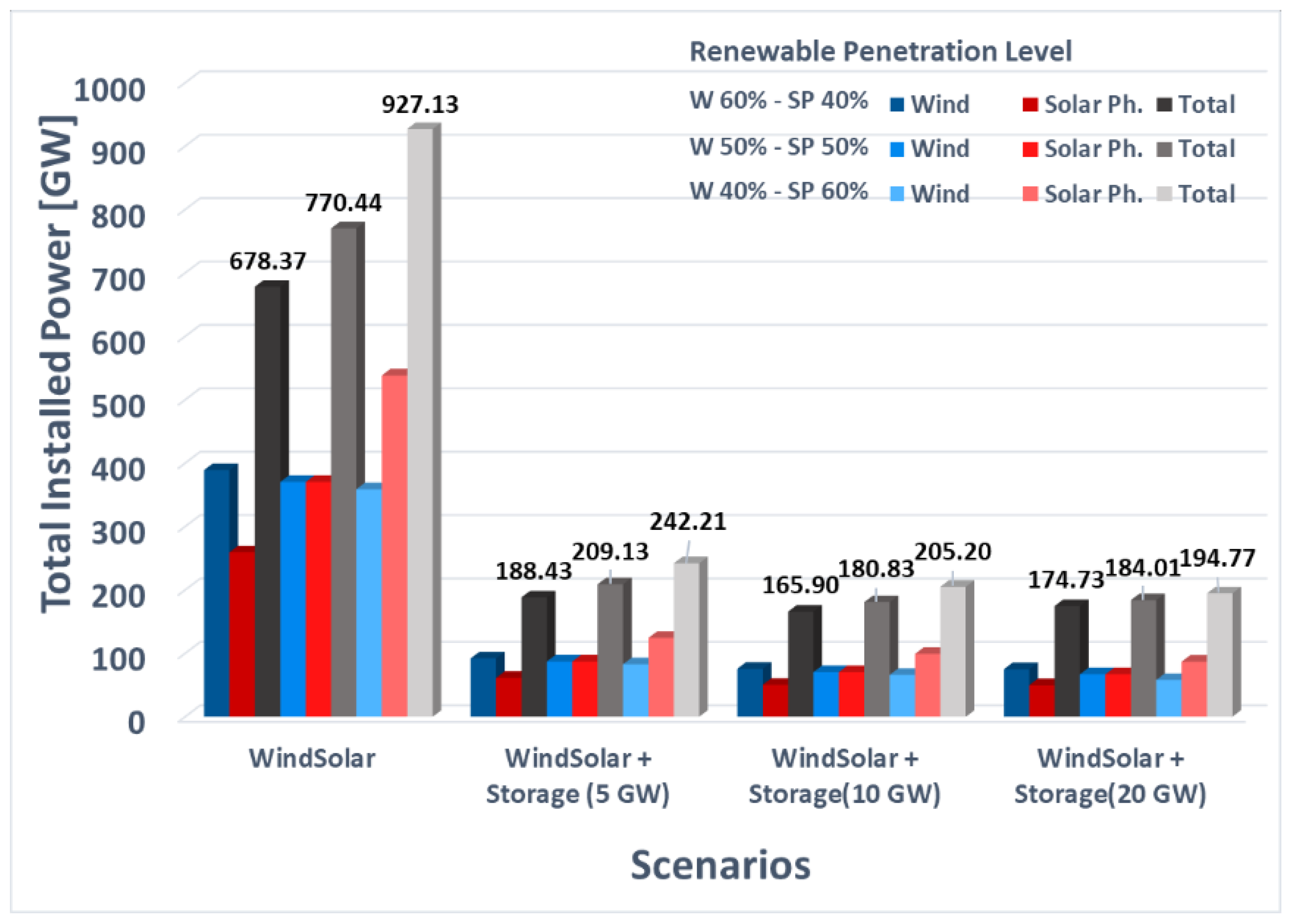
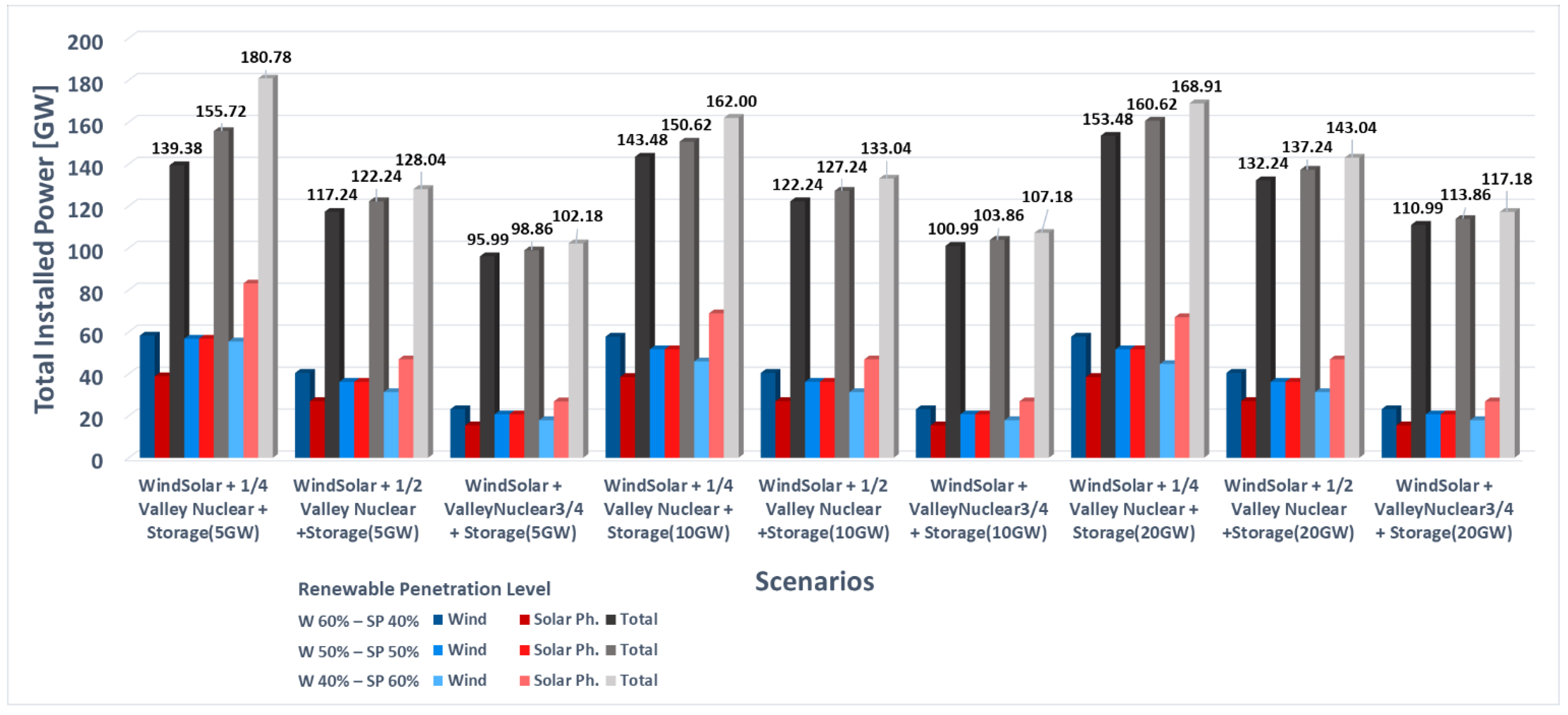
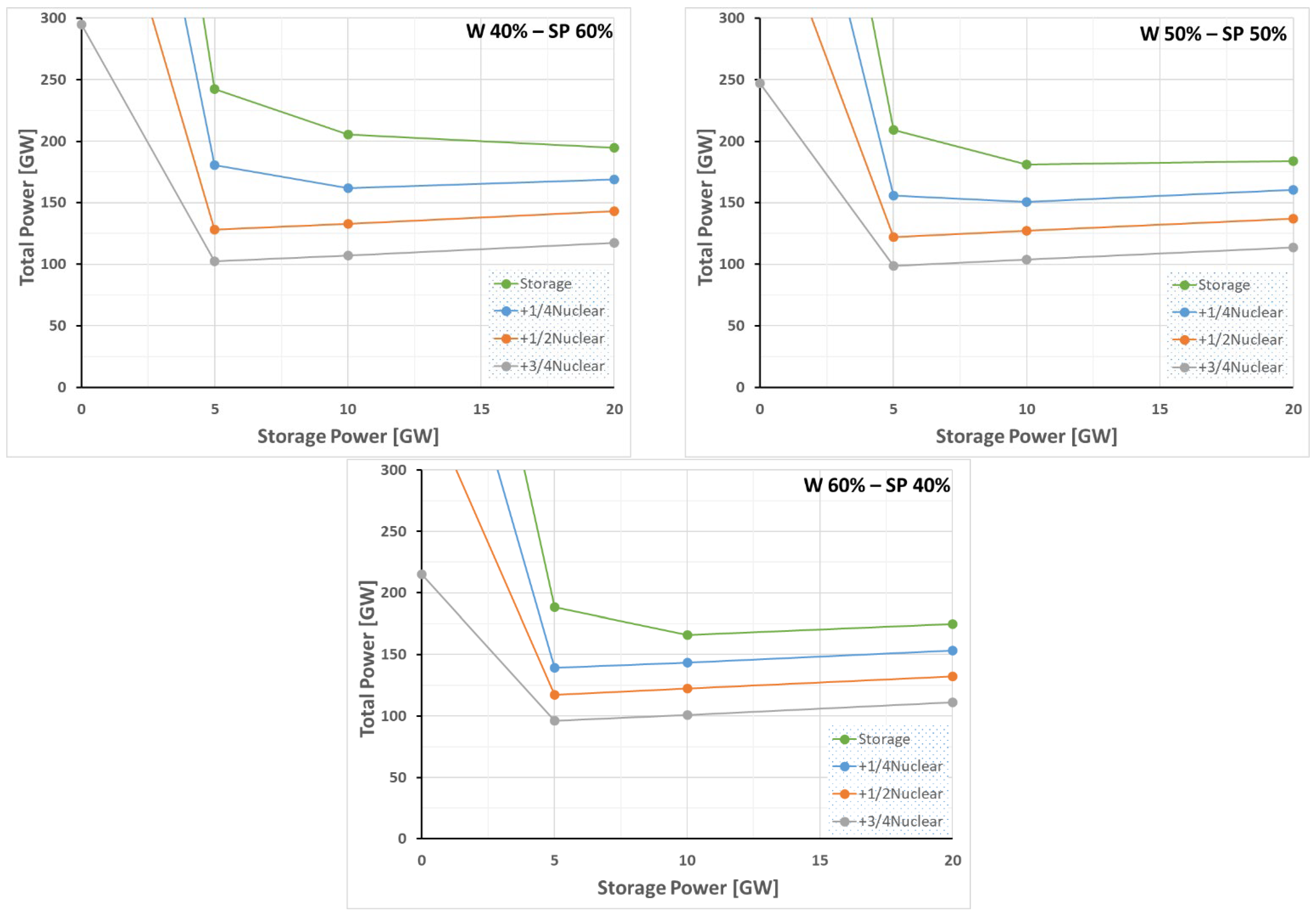
Power (GW) for each Renewable Penetration Level
(Wind-Solar Photovoltaic in %)
W 40%–SP 60%W 50%–SP 50%W 60%–SP 40%
Monthly Averaged 1174.8164.0154.7
Daily Averaged268.6222.4191.1
Monte-Carlo927.1770.4678.4
1 Equilibrium in the monthly averaged balance between generation and demand (constant generation and demand, only the capacity factor of each generation source is considered), extrapolation of REE’s February 2017 data to year 2040.
Table 6. Summary of wasted electricity values depending on the renewable penetration and generation scenarios (pure renewable, renewable with support of nuclear and/or storage).
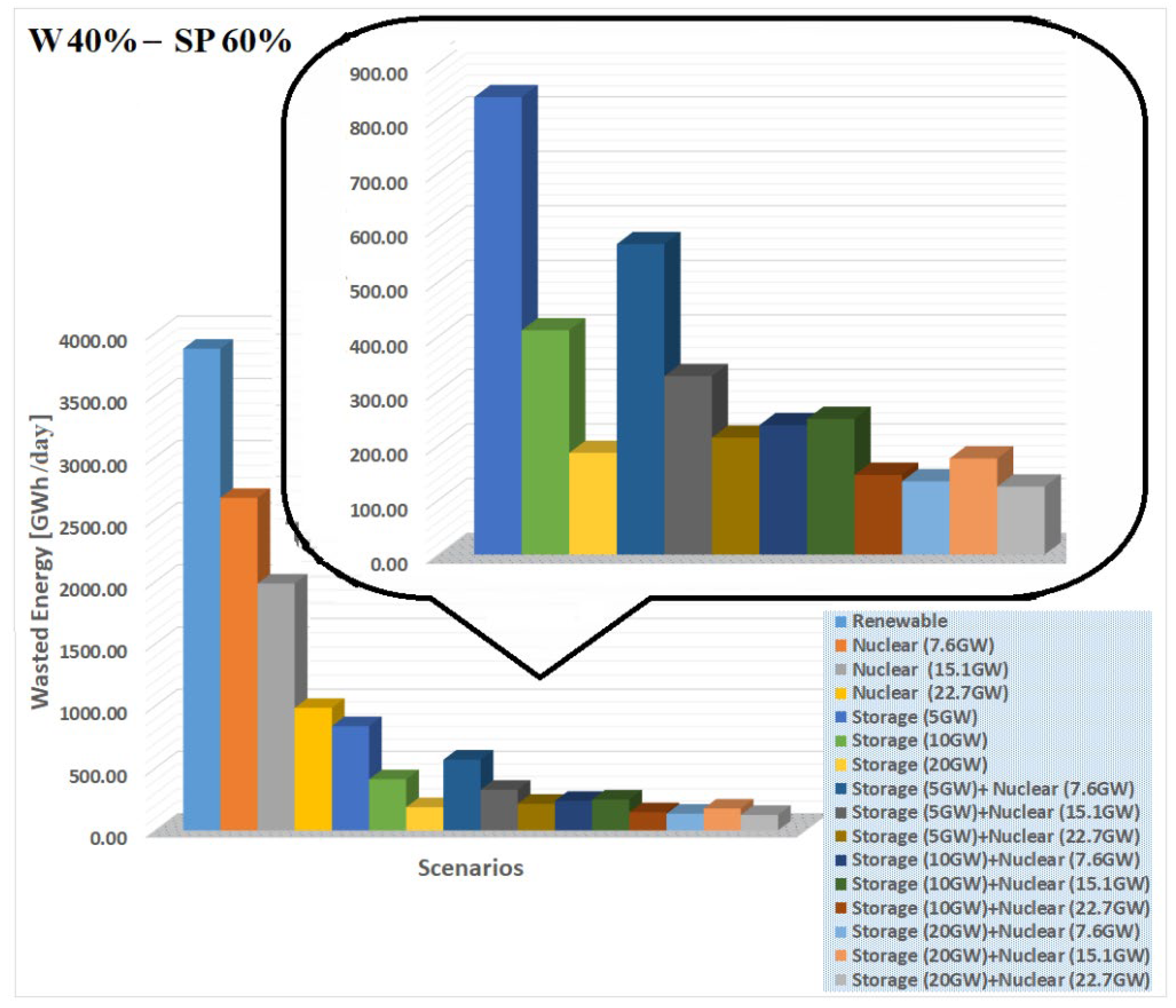
Daily Wasted Energy (GWh) for Each Renewable
Penetration Level (Wind-Solar Photovoltaic in %)
W 40%–SP 60%W 50%–SP 50%W 60%–SP 40%
Pure Renewable387334253216
Plus NuclearCurrent Power267325972570
Upgrading x 2198517311609
Upgrading x 4985947920
Plus StorageCurrent Storage839666579
Upgrading x 2411296247
Upgrading x 4186175173
Plus
Nuclear and Storage
Current Values569521507
Storage upgrading x 2237303398
Storage upgrading x 4134209286
Nuclear upgrading x 2327321323
Plus Storage upgrading x 2249239239
Plus Storage upgrading x 4176170169
Nuclear upgrading x 3214264311
Plus Storage upgrading x 2146184221
Plus Storage upgrading x 4125151174
Publisher’s Note: MDPI stays neutral with regard to jurisdictional claims in published maps and institutional affiliations.

