An Energy-Fraud Detection-System Capable of Distinguishing Frauds from Other Energy Flow Anomalies in an Urban Environment

Abstract

Energy fraud detection bears significantly on urban ecology. Reduced losses and power consumption would affect carbon dioxide emissions and reduce thermal pollution. Fraud detection also provides another layer of urban socio-economic correlation heatmapping and improves city energy distribution. This paper describes a novel algorithm of energy fraud detection, utilizing energy and energy consumption specialized knowledge poured into AI front-end. The proposed algorithm improves fraud detection’s accuracy and reduces the false positive rate, as well as reducing the preliminary required training dataset. The paper also introduces a holistic algorithm, specifying the major phenomena that disguises as energy fraud or affects it. Consequently, a mathematical foundation for energy fraud detection for the proposed algorithm is presented. The results show that a unique pattern is obtained during fraud, which is independent of a reference non-fraud pattern of the same customer. The theory is implemented on real data taken from smart metering systems and validated in real life scenarios.

1. Introduction

Electricity and energy (including water, gas) fraud detection is an intriguing subject which has gained a high level of interest in recent years. Energy fraud detection is important for urban ecology and not only for supplier’s finance; the reduction of energy losses results in less generation. Less energy generation and transportation mean a reduction in carbon dioxide emissions, and better urban energy grids planning in the wide sense: electricity, water and gas. The research presented herein is implemented on electricity data but can be suitable to gas and water data with replacement of the training datasets. According to a recent annual document regarding smart metering benchmarks published in December 2019 [1], the detection of electricity technical and non-technical losses results in vast operational benefit. The report indicates that, in Europe, 7.5% of energy is lost in the distribution grid due to technical and non-technical losses, and an additional 7.5% of losses are encountered in the transmission grid. According to the survey in [2], electricity fraud results in 89.3 billion dollars of loss annually, 58.7 billion dollars of which are in the emerging markets. According to a report published in October 2017 by the Council of European Energy Regulators (CEER) [3], the distribution losses due to technical and non-technical losses are in the range of 1% (in Iceland) up to 14% (in Malta), and, on average, are 7.5%. According to an earlier work by T. B. Smith from United Arab Emirates (UAE) [4], the losses in the Western Europe Transmission and Distribution (T&D) grid were about 7.56% in the year 2000. The numbers reach as high as 14.6% in Africa, and an average of 16.2% worldwide [4]. The cost-savings upon operation of fraud detection mechanisms are significant [4]. Existing algorithms for fraud detection are usually operating on electric energy load-profile data. These data are periodic with a quarter-hourly up to hourly registration of energy consumption in that period. These data are attained by a smart meter and may represent one of four quadrants: active energy and reactive energy, where each can be either import or export. The common theme of most, if not all, fraud-detection technologies is feature generation, whether human or automatic, that enables distinguishing between fraud and non-fraud. This survey presents meta-families of anomaly detectors which, within themselves, include a large family of architectures. A key component to many of the presented architectures is the autoencoder. An autoencoder performs some operation over the data called $\widehat{P}$. The next operation performed is inverse operation ${\widehat{P}}^{-1}$. The network over the data is the identity operator $\widehat{I}={\widehat{P}}^{-1}° \widehat{P}$. Hence, the outliers are excluded from the dataset. Reducing the “only normal” items from the entire dataset is the “outlier dataset”. Autoencoder implementations exist in various machine learning architectures, and they are the first meta-architecture in fraud detection. The second meta-architecture in fraud detection is the classifier between fraud/no-fraud. This requires a preliminary feature generation module to enable distinguishing between the two clusters. A work on cascading of Convolutional Neural Networks (CNN) and Gate Recurrent Unit (GRU) was performed by U. Ali et al. [5]. The cascaded CNN-GRU algorithm reaches an average of 87% detection without the Manta Ray Foraging Optimization (MRFO) back-propagation algorithm, and up to 91% with MRFO. CNN and GRU are both deep learning algorithms and therefore require large amounts of load-profile data, and a large fraud detection dataset. A survey by Guo et al. [6] covers classical machine learning classifiers, such as a support vector machine (SVM). Ullah Shoaib et al. use, again, the CNN-GRU network, this time with the Particle Swarm Optimization (PSO) back-propagation optimization algorithm [7]. The work performed by Kim et al. [8] is, again, investigating a dual cascaded CNN-LSTM (Long Short-Term Memory) network, and near-global weight optimization back-propagation algorithm. The work by Kim et al. [9] implements the Generative Adversary Network (GAN) for anomaly detection through an auto-encoder. Korba et al. [10] implemented an electricity fraud detection algorithm using “Support Vector Machine” (SVM) which requires feature generation and is used occasionally as a classifier. The SVM increases the features that dimensional space variables count, thereby making fraud/non-fraud clusters further away and easier to classify. Yue et al. implemented a cascade of nonlinear classifier decision trees and SVM [11]. Tumen et al. implemented the LSTM fraud detection algorithm [12], which excels the anomaly detector but does not automatically generate features [12]; therefore, there is a data selection module which attempts to select some data. Ahmed et al. [13] implemented two algorithms that handle the issue that fraud data are imbalanced data. The authors use Python imbalance handling library SMOTEENN which performs oversampling by the SMOTE function and cleaning using ENN: “synthetic minority oversampling technique with edited nearest neighbor” [14]. The SMOTE is a technique for data augmentation for the minority and was invented by Nitesh Kawla. William Eberle et al. [15] simply implemented a neural multi-layer perceptron (MLP) as an anomaly detector. Mishra et al. [16] published a study with a cascaded two levels of classifiers, Decision Tree (DT) and “Support Vector Machine” (SVM), acting as an anomaly detector. Another work implementing CNN is by Zhou et al. [17], utilizing the features generated by preliminary convolution layers into an anomaly detector. Another method is implemented by Zhao et al. [18] with CNN-RF, RF means random forest. Here, again, the minimal pre-processing of measuring distance is performed for anomaly enhancement, then it is inserted into the CNN and then into the RF. It is important to notice that the initial dataset is imbalanced, and, via the SMOTE algorithm, it becomes balanced. A comparative work by Wang et al. [19] developed the concept of an unsupervised autoencoder-based ensemble method for anomaly detection. The performance of various autoencoder types and training schemes is compared there. In the work, methods are developed for performance quantitative evaluation of fraud detection algorithms. Work performed by Duarte et al. [20] computed human generated features which tend to be entire-data collaborative. This time-series data are injected into simple AI structures, such as Pearson correlation heatmap, and obtain a distinction between normal and abnormal images. The innovation here is in feature generation and less in artificial intelligence architecture; however, it is important in the sense of the possibility of visualizing fraud simply by generating load-profile data collaborative features. Another comparative work by Hatziargyriou et al. [21] presents a fine categorization of electricity fraud detection algorithms. This work is an in-depth review, providing insights into the entire volume of fraud detection implemented methods and their classification. According to this work, the machine learning is categorized into “data oriented”, “network oriented” and a hybrid of both methods. Data oriented is based on feature generation and imbalanced data balancing algorithms. Network oriented methods require the use of power grid data (network topology network measurements). The insights of this work are too wide to describe in a literature review. The work by Joshi et al. [22] cascades the SMOTE imbalanced data balancing technique to a secondary layer of the Principal-Component-Analysis (PCA) method. PCA is a matrix transform, reducing high-order-dimensional space dimensionality into the desired dimensions count, thereby excluding the dataset members located outside the main clusters. These are called the outliers. KPCA (Kernel Principal Component Analysis) is the kind used in that paper as a feature extractor. Almost no works were performed on reducing false positive detection, yet the general approach of reducing false positive in frauds is studied systematically in fraud accounting [23]. There, the conclusion is to use a different algorithm, and not to use the fraud-detection algorithm positives the same way. Electricity fraud detection reduction of false positives is discussed in [24]. When speaking of suitability also to industrial premises, there are not only conventional grids, but also second-generation power components, such as a loss-free resistors [25] and gyrators [26].

The works described above present a wide spectrum of methods. Three gaps can be identified in descending importance, and they are all correlated to the question of: how robust shall an algorithm really be in field conditions? The first proposed gap is the need to define features that reflect “energy consumption expert knowledge” and “entire data collaborative” and redirect the training by the clustering AI core as improved training in the sense of training time, accuracy and requiring less data. The second gap is the practice of the algorithm in field conditions within a utility company. The potential answer is that there is a set of non-fraud anomalies that appear to be fraud [27,28] and, in order to reduce the fraud false positive, it is required to know how to separate them from the cases suspected as fraud in the office level. Another issue of this work is to present this as a matter of conditional probabilities and confidence level computation prior to sending qualified fraud detection personnel to the field. Identifying these anomalies and pointing out algorithmically how to filter them is the second gap and the proposed solution. The third and last gap follows in order of importance. At infancy stage not too many verified frauds, and role of additive clustering models shall be investigated [29]. A question has arisen as to what the internal mechanism is of the algorithm proposed herein, and whether the other algorithms in other works encounter the same anomaly phenomena in a similar way. Could that be answered on a theoretical computational ground? The comprehension of the fraud signature in high-order dimensional space and through 3D principal component analysis (PCA) transform shall be inspected through a series of “vector space and linear algebra and statistics” theorems. The research shall investigate what is the comprehension of the suggested features capability to distinguish between fraud and non-fraud. For the proposed solution, there is a pattern that repeats itself in all solution sub-spaces. Is it likely that other algorithms encounter the same phenomena reported in this work? Other anomalies that reside in a closer location in high-order dimensional space, therefore, look similar to fraud. Returning to the issue of conditional probabilities, the algorithm’s holistic nature is a requirement drawn in light of its operation in the field. The mathematical foundation (issue 3) is necessary in order to comprehend the physics of the suggested solution, and to investigate what is the likelihood of other algorithms to experience the same phenomena encountered by the research group. With regard to the dataset, there are internationally published datasets. Due to un-tagging of non-fraud cases in “fraud detection datasets”, only through trial and verification at a local utility company can an algorithm be trained to distinguish between anomaly cases. This paper uses extensively a local utility company anonymous tagged training dataset. A local distributed system operator (DSO) testing dataset of two-hundred meters was established and suspected frauds were tested in the field, while some frauds were emulated on real meters in the field, such as magnetic tampering, phase disconnects and phase reversal. The algorithm is dynamic and iterative, as the algorithm starts to work, more cases are verified, and the training ‘fraud tagged’ dataset becomes available. Another issue is the ability to detect fraud when there is no reference of non-fraud behavior concerning the suspected customer. A notification of other anomalies that are more differentiated are: (I) defected data in the smart metering data chain from meter to data warehouse. This problem is demonstrated by the paper as crucial through examples given. It is almost certain that it prevails in other electricity fraud detection algorithms. A “data mismatch in the smart metering information chain”, “detector and allocator” sub-algorithm of the electricity fraud-detection shall be briefly presented. Without it, the data mismatch show as an anomaly and may be accidentally identified as suspected fraud. (II) The second type of grid anomalies that are not fraud are related to preventive-maintenance and cyber intrusion detection, and these should also be presented; there are nations that are occasionally cyber attacked. Consequently, in a previous work by this group [30], a reference is presented, and it is assumed differentiated herein that these anomalies are separated. (III) There are several methods of electricity fraud such as: magnetic tampering, phase reverse and phase disconnect or consumption biasing the phase. It is advantageous that the algorithm may work as a classifier of tampering types and not only as an anomaly detector. The sixth gap identified is the current-state modularity of the algorithm for future enhancement. There are several additional future information sources that modify the false positive accuracy.

There are training data and datasets such as for example [31,32].

In this paper, we will show a new method for electricity fraud detection at the entry to the premises. The method is based on electricity fraud-detection by a generation of a new set of strong energy-consumption trend “data collaborative signature” features. These features exceed the following set of “differentiating load-profile value from average” works. These rules constitute the preprocessing layer. The paper shall describe three groups of rules, ensuring that each is “collaborating the entire load-profile periodic data” electrically and statistically, proving a panoramic electricity business view of the customer profile. In addition, the paper shall include the development of a theory of electricity fraud-detection specific to the proposed algorithm and universal to all algorithms. Gaps (1)–(6) presented above are all addressed using a single theme. The proposal uses only load-profile data. The algorithm generated 256 statistical parameters, providing the customer panoramic view of fraud/non-fraud speaking. The AI is sophisticated enough, using a correlation heatmap to fraud/no-fraud, in order to reject 156 parameters, leaving only the meaningful data. Computation cost is low: 5–10 min over a single processor, with up to five years of historic load-profile. In order to obtain high accuracy, the proposed algorithm uses a fraud detection data-augmentation assisting algorithm. The low computation cost enables personalized training, because a single server may train over 50,000 customers/year.

2. Materials and Methods

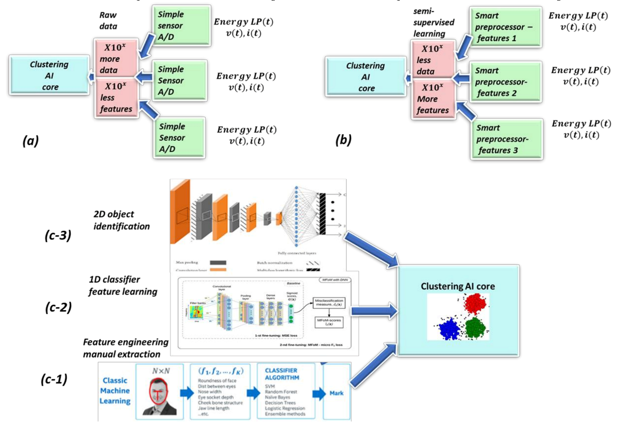
2.1. Proposed Architecture

Figure 1 presents the algorithm architecture in the format that is common to other works. It presents the primary goal of the paper: utilize electro “consumption-trend” knowledge to better cluster fraud and non-fraud. This is the paper’s most important contribution: the energy consumption-trend features demonstrate very clearly the difference between fraud and non-fraud and show the “physics of electric consumption”. The second module is a supervised learning clustering core that is used to ensemble learning, partly in order to learn about and to research the performance, and partly because it shall be shown that different algorithms outperform others which are dependent on the maturity of the dataset. The local DSO (distributed system operator—entity deploying smart meters and collecting data for distribution to suppliers and customers) section of the training dataset is dynamic and increases with time. The classification core would be enhanced if replaced in the steady-state period, when sufficient data are gathered, by the CNN object identification module, as presented in the future research section. The effect of the pre-processing feature generation is the most important—it is modular, and it shall be shown in the Results section, and “Materials and Methods”, that it acts similarly to the 2D facial recognition system. Consequently, it is capable of identification of fraud-types (tempering magnet, reverse phase, phase disconnect) and of other anomaly types disguised as electricity fraud, such as maintenance/configuration/communication mismatch. Figure 1a represents a conventional fraud detection architecture, where input to clustering AI core is raw data. Figure 1b represents the proposed architecture where the front-end smart preprocessor constructs a high-order dimensional space that redirects the training.

Figure 1c: front end is modularly connected to a different clustering core during the lifespan of the algorithm. It shall be shown that, at “infancy”, the post-installation stage at a local utility company, the logistic regression, which is a Generalized Additive Model (GAM), converges fastest over 10–15 local utility verified frauds. There are international datasets [21], however, as shall be shown, they do not contain tagged non-fraud anomalies. Therefore, additional verified frauds and anomalies from local DSO are added. In the first maturity stage, when there are already ~100 verified frauds, random forest (RF) and decision tree (DT), non-linear classifiers are shown to be more accurate and converge well. During the latest maturity stage, which is not implemented yet, several deep learning algorithms fit: these require an order of ~${10}^3$ verified frauds. Currently, RF and DT act as clustering algorithms and they perform this well with much fewer test cases. It shall be shown herein that generated consumption knowledge features are 2D. A regular CNN/LSTM classification core is possible. This is heuristically shown in 1-c-2 as the middle 1D CNN. The generated features are $y=f\left(x\right)$ or, stated differently, $f\left(x,y\right)=0$. This is represented as 1-c-1. It shall be shown in the Results section that human cognition may distinguish fraud from non-fraud through the presented features. Therefore, a 2D CNN for object identification shall excel in classifying various anomalies from fraud and various fraud types. This is shown in 1-c as upper 2D CNN, such as heuristically illustrated at 1-c-3. However, the proposed front-end is successful in the generation of distinguishable patterns in high order dimensional space, and DT and RF are sufficient for clustering them; they are implemented in this research. What is important is that front-end high order dimensional space is modular and is currently demonstrated with five classical machine learning algorithms but may also re-direct training with deep learning algorithms 1D and 2D object identification.

2.2. System Flow Diagram—At Distinguishing Various Anomalies Level

Figure 2 presents the flow diagram of the core algorithm lower-level design. This relates to the paper’s secondary contribution. The proposed algorithm is different than most presented algorithms in that it is holistic. It shall be shown in the theoretical math, Section 2.8, and through examples in the “Results” section, that various anomalies reside in the high order dimensional space, adjacent to the fraud cluster, and most likely in other presented works as well. If not separated, it shall be shown that in practical field conditions, they significantly increase the false positive rate. The presented anomalies 2.1–2.6 cover the majority of false positives: preventive maintenance, grid cyber intrusion detection and data mismatch in the smart metering/grid data chain. Additional probability interference is derived for some smart meter models through built-in events of (1) magnetic tampering and (2) meter front panel opening. If they do not exist, then the algorithm ignores them, however, if they do, then their trigger dramatically affects the confidence level of actual fraud. Item 2.4 presents a non-implemented, as of yet, module, still of considerable affect over the confidence level, and that is “customer information” deriving from the customer information database. The solution should be modular to operate even without such a module. A description of future work architecture and the technology it shall utilize is presented in the Chapter of Future Work. Examples of customer information are address, socio-economic class and indication of person abroad/not-abroad. The last affecting factor is item 2.5: super-consumption. Fraud detection in previous works usually means fraud from the supplier or sub-consumption. There is another type of fraud that is of security interest, fraud from another customer, and that is 2.6. super-consumption. Super-consumption shall be shown at Results at Section 3.10.

2.3. An Ever-Learning Algorithm Flow Diagram

Figure 3 presents yet another layer of the proposed algorithm, supporting the presented approach of a holistic solution. The algorithm presented in Figure 2 is iterating over itself as presented by Figure 3, enriching the local training dataset both with additional fraud/non-fraud samples and new classes. The anomalies filtered out by this paper’s presented algorithm section may be tagged in the maturity stage by the original presented fraud detection algorithm also, and that shall be shown in the data mismatch anomaly in the Results section. In addition to being identified at maturity stage by AI algorithm, they are during entire lifetime, interrogated by the robotic process automation software described at Section 2.14.3 Figure 12 further on. Claiming that other algorithms are likely to encounter the same anomalies misidentified as fraud in the proposed algorithm should be based not only on our word, although it is permissible. There are works about grid anomaly and works about fraud detection. These are merged in our presented work. However, a considerable mathematical section is presented in order to be able to state exactly that. The focus of the paper is that it presents the core algorithm mostly, however, it relates with AI architecture exactly to the additional phenomena. Not as a best practice, but as precise algorithms. In the discussion below, energetic consumption recorded in a period is assumed non-aggregative. If, at a specific smart meter, the energy recording is aggregative, it is easy to transform to a non-aggregative load profile.

2.4. Group One: Energetic Distribution from Load-Profile

The first group of engineered features is derived from taking the electricity load-profile and generating bins of energy distribution:

$$\begin{array}{cc}& n\left(E_m\right)=\frac{n(E_n\le E<E_n+\Delta E)}{{{\displaystyle \sum }}_{m}n\left(E_m\right)}\hfill \\ & n\left(E\right)={\lim }_{\begin{array}{c}N\to \infty \\ \Delta E\to 0\end{array}}count\_of(E_n\le E<E_n+\Delta E)/{{\displaystyle \int }}_0^{\infty }n\left(E\right)dE\hfill \\ & n\left(E\right)={\lim }_{\begin{array}{c}N\to \infty \\ \Delta E\to 0,E_m\to E\end{array}}n\left(E_m\right)=\frac{{\lim }_{\begin{array}{c}N\to \infty \\ \Delta E\to 0,E_m\to E\end{array}}n(E_n\le E<E_n+\Delta E)}{{{\displaystyle \int }}_0^{\infty }n\left(E\right)dE}\hfill \\ & N={{\displaystyle \sum }}_{m}n\left(E_m\right)\hfill \end{array}$$

(1)

where:

$n$—number of load-profile periods counted with energy that is inside the bin [$E_n,E_{n+1}]$;

$N={{\displaystyle \sum }}_{m}n\left(E_m\right)$—entire load-profile periods count, which is a summation over all bins of periods counts. It is not the entire energy, the formula for the entire energy is ${{\displaystyle \sum }}_{m}n\left(E_m\right)E_m\Delta E$;

$n\left(E\right)$—a limit continuous function of the series $n\left(E_m\right)$ at the point $E_m$when the periods count N becomes infinite and the bins split $\Delta E$ becomes zero;

The latter limit $\Delta E\to 0$ cannot be performed without incrementation of N, otherwise the digital distribution shall not reflect the true distribution because there shall be empty bins which do not occur as of yet.

The figure $\Delta E\ast N$ can be made to equal a constant. Meaning:

$$\Delta E\cdot N=E_{max}$$

(2)

where:

$E_{max}$—consumer maximal energy of consumer per period, meaning the period is defined as quarter hourly up to one hour.

The distribution function of a characteristic consumer, let it be rural, residential or industrial, as depicted in Figure 4: a comparative visualization of the distribution function defined by Equation (1) between three verified frauds and three verified non-frauds.

Characterizing what is observed, the following guidelines may be outlined by observation of Figure 2.

The three verified non-frauds and the three verified frauds are a sum of two/three normal distributions. A consumer has a maximal energy consumption, and around it the law of large numbers prevails, meaning normal distribution. There are two or three peaks in the day dictating three normal distributions. Figure 1 is not a daily distribution, but is actually:

$$n\left(E\right)={\displaystyle \sum }_{i=1}^K{\phi }_{i}N\left({\mu }_i,{\sigma }_i,h_{max,i}\right)$$

(3)

where:

$N\left({\mu }_i,{\sigma }_i,h_{max,i}\right)$—normal distribution with matching average, variance and peak height.

The normal distribution is characterized by three parameters:

$$\begin{gathered} N\left(\mu ,\sigma ,h_{max}\right)=\frac{h_{max}^{’}}{\sqrt{2\pi \sigma }}{e}^{-\raisebox{1ex}{${\left(E-\mu \right)}^2$}\!\left/ \!\raisebox{-1ex}{$\left(2{\sigma }^2\right)$}\right.} \\ \frac{h_{max}^{’}}{h_{max}}=\sqrt{2\pi \sigma } \end{gathered}$$

(4)

where:

$\mu =E_{central,i}$—normal distribution central energy with peak consumption share of total time;

$h_{max}=N\left(E=\mu \right)$—peak count of periods at most common energy value of the specific normal distribution. Th is the consumption periodic energetic value that is most common;

σ—variance. The width $\pm 2\sigma$ around central energy where 68.26% of periods are. The width edge points are determined where $N(E=\mu \pm \sigma$)$=h_{max}/2$:

• The distribution is distinctive in terms of mathematical formulation between fraud and non-fraud. The right-hand side of Figure 2, representing verified non-frauds, is a sum of normal distribution, where for each distribution the maximal height is larger than the width. The height is a maximal count of bins per specific energy value $E_n,$ or alternatively stating “energy bin value”$\left[E_{n,},E_n+\Delta E\right]$. On the other hand, observing all verified frauds, the maximal height is smaller than the half probability width. This rule was tested for a very large count of frauds and non-frauds and is always correct. On its own, it is insufficient for reliable fraud detection. The fraud customer is “shaving the peak”. The clustering into fraud/non-fraud shall be performed using AI and not some $h_{max}/\sigma <>1$selection rule.
• Behavior is collaborative, assuming Figure 2 is generic and that it is based on large cases count. It reflects the entire load-profile, and the litmus test is that by observation it is possible to initially mark suspects of electricity fraud versus non suspects.
• Rule 1 of suspected fraud detection is correct even without a reference of non-fraud for that same customer. A customer may start stealing from day one and disguise themselves as a low consumption customer, yet the statistical energy distribution signature cannot be tricked. There is one exception. Anomaly due to data chain fault may look similar, and that is similar to other features by other algorithms as well. It shall be shown within the paper how this may be resolved. This means that there is no requirement for reference of non-fraud from that same customer, and that is innovative as compared to most fraud-detection algorithms.

Normalization: in order to enable learning from one consumer of $5000 \mathrm{kilo}-\mathrm{Watthour}/\mathrm{year}$ to another consumer of $50 \mathrm{killo} \mathrm{Watthour}/\mathrm{year} ,$as much as can be learned, at least for not too far apart consumption profiles, the distribution is normalized just before construction of the high-order dimensional space. This is a simple and most powerful tool that enables comparison between any two customers. Independently, Group 1 is an insufficient level of confidence for determination of suspected electricity fraud. The required confidence level must be at least 95% true positive and less than 5% false positive.

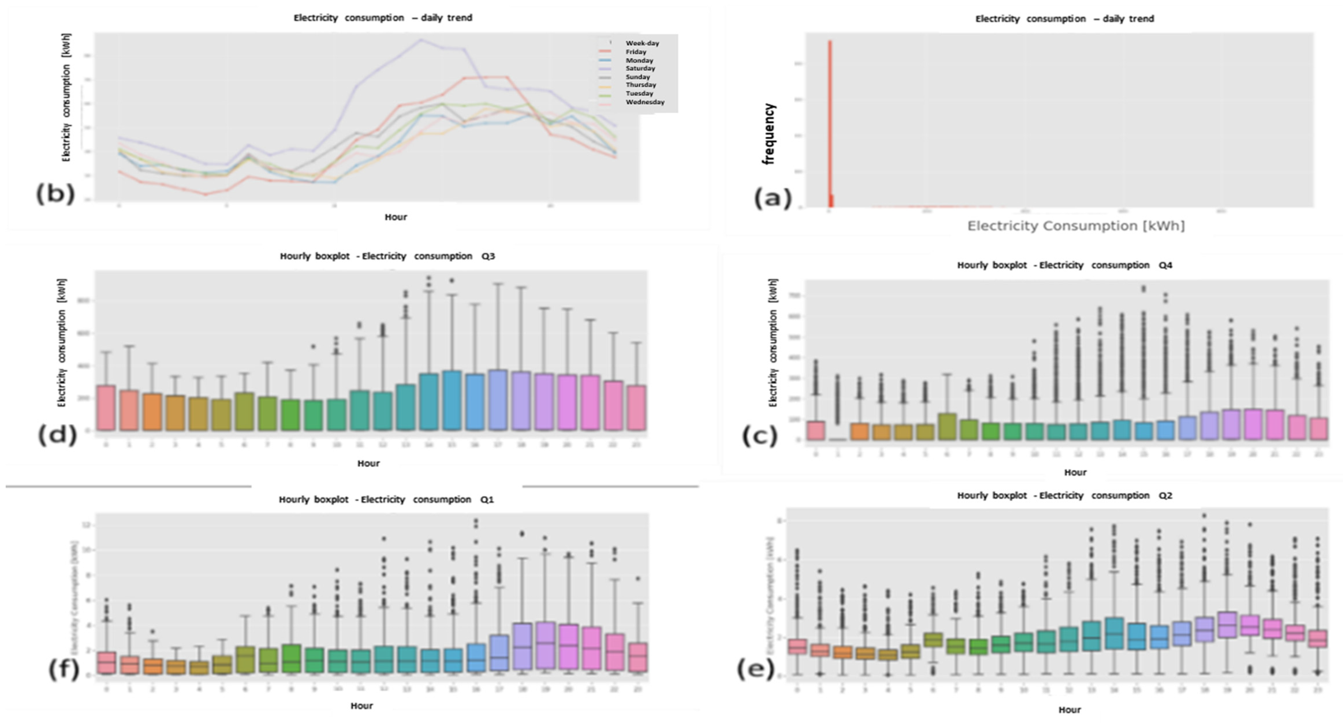
2.5. Group Two: Daily Hourly Trends Computed from Load-Profile

Another collaborative feature is to take an entire energetic load-profile constructed of periods and, for each day, calculate the average trend hourly energetic consumption curve. This may also be performed seasonally as a daily–hourly trend. Herein, we focus on daily–hourly trends without seasonal separation. For which the mathematical formulation is:

$$E_{day\left(i\right)}\left(t’=t_n\right)=\frac{{{\displaystyle \sum }}_{period\in t_n}E\left(t’=t_n\right)}{N}$$

(5)

where:

$day\left(i\right)$ $\in \left(Sunday, Monday,\dots ,Saturday\right)$

$t_n$—each day is constituted of a fixed number of recorded energetic periods and fixed period times. For example, a quarter hourly load profile: 00:00, 00:15, …, 23:59; there are 96 quarter hourly periods. $t_n$ is a fixed time occurring each day. For example: $t_n=12:15$.

$period\in t_n$—summing all periods from each and every day, one period per day of time $t_n.$ For example, $t_n=12.15$.

N is the total number of days within a recorded load profile which equals a total number of periods $t=t_n.$

$E_{day\left(i\right)}\left(t^{\prime }=t_n\right)$—average energy in day of week $day\left(i\right)$, of type defined above. Averaging is over all periods of historic energetic load profile.

Figure 5 describes “daily–hourly” trend graphs of days of the week $\left(Sunday, Monday,\dots , Saturday\right).$ Certain customers consume the same during weekends as the rest of week, such as factories. With regard to other customers, there is either a decline during the weekends—such as “workplaces”, or a rise during the weekends—such as in residential premises.

Figure 5 is characteristic to all fraud and non-fraud cases. It was repeated for hundreds of verified non-frauds and tens of verified frauds. The following characteristic behavior is observed. For verified non-fraud, there is strong regularity of daily curves and equalities of daily curves, at least for regular “weekdays”, Monday–Friday. For verified frauds, there is a mess with trends, and, in addition, they are not close to each other. The feature is collaborative, it generates a classifying fraud/non fraud signature for all customers. Regardless of the fraudulent person disguising themself as having a low-consumption rate, he cannot escape the statistical signature of Figure 5, right hand side. This means that there is no requirement for reference of non-fraud from that same customer, and this is innovative as compared to most fraud-detection algorithms. The signature may be characterized by measurement of the collaborative RMS distance between any day to any other day and taking the maximum of these RMSs. Normalization: there is no single customer with exactly the same consumption, or even the same normalized consumption profile. Therefore, the distance between the shapes is normalized by shape absolute value.

2.6. Group 3: Seasonal Hourly Boxplot Graphs

The third and last features group is seasonal–hourly boxplot graphs. Taking separate periods belonging to one of four seasons and generating a boxplot of the hourly energy consumption is the initial definition of a boxplot. Figure 6 illustrates, per a specific season, the boxplot as a mapping of normal distribution of a cluster of samples. In group 3, that is the periods referring to the same time moment, taken from the entire load profile and not of the same date.

The hourly boxplots generate a full entire load profile view. The boxplot was introduced by M. E. Spear in 1952 [33] and again in 1969 [34] It is an effective tool for panoramic display in terms of, for example, normal distribution. There are, of course, recent references [35], and the boxplot has become a standard Python object in three libraries, seaborn, matplotlib and pandas. Boxplot outliers are exceptions to the normal distribution within the 0.1% of edges. The collaborative entire data view does not complete with a single boxplot. There are twenty-four boxplots per twenty-four hours per day. Therefore, there may be up to $24\ast 7=168$ sub-features in group 3, providing a collaborative view of the entire load profile data per season over several years. For four seasons there may be up to $4\ast 168=672$ features per group 3.

Dimensionality reduction: on one hand, this is a panoramic view. On the other hand, this may be too many dimensions, in terms of contribution to fraud detection. With regard to efficiency, the software computes the Pearson correlation heatmap between all parameters to all, and especially to fraud, and about 61% are not correlated to fraud and removed. The Pearson formula is:

$${\rho }_{x,y}=\frac{cov(x,y)}{{\sigma }_x{\sigma }_Y}={\displaystyle \sum }_{i=1}^n[\left(x_i-\stackrel{-}{x}\right)\left(y_i-\stackrel{-}{y}\right)\left]/\right[\sqrt{{\displaystyle \sum }_{i=1}^n{(x_i-\stackrel{-}{x})}^2}\sqrt{{\displaystyle \sum }_{i=1}^n{(y_i-\stackrel{-}{y})}^2}]$$

(6)

where:

${\sigma }_x,{\sigma }_y$—the standard deviation of$x,y$;

$x_i—$object instance forecast;

$y_i—$object instance actual.

This function computes the correlation between these object instances, thereby revealing correlation in accordance with a specific classification algorithm. The Pearson formula is a built-in Python function, it generates a correlation heatmap and is a method of library scipy class stats.

A characteristic comparative view of a seasonal hourly boxplot, fraud verified (upper) and non-fraud verified, is shown in Figure 7.

It is visible that the upper outliers count in a verified fraud example is much larger than the verified non-fraud case. The boxplot carries much more information than that, and therefore it is studied as 165 variables per season. We may even draw a connecting and imaginary line between all boxes upper front of $+25\%$ (point 7 in Figure 6), and an imaginary line connecting between all boxes, lower boundary $-25\%$ (point 3 in Figure 6); an imaginary wavefront is observed and even that collaborative feature may be investigated. Since especially group 3 generates 168 parameters times four seasons (672 features overall) and the Pearson correlation heatmap reduces 60% of features, the three groups act similar to a 2D facial recognition system of three sets of systems: $f_i\left(x,y\right)=0$ where $i$ is group index. However, there are no faces herein, there are fraud/non-fraud consumption all-data collaborative patterns. This is heuristically demonstrated in Figure 1c middle function. It shall be shown why the algorithm is successful in many abnormal ‘classification procedures’, and is performance compatible with CNN, only with much less data.

2.7. Group 1: Energy Distribution Feature Extraction and Construction of a High-Order Dimensional Space

A high-order dimensional space is constructed according to the model of Equations (3) and (4). There are built-in algorithms that best fit a sum of two to three Gaussians: Gaussian Mixture Model (GMM) described by Raynolds [36] and Kernel Density Estimation (KDE) with Gaussian kernel. KDE is most common, for example, with deep neural networks where there are numerous works. A tutorial material on GMM method is shown in [37].

From these systems, regardless of how they operate, results have in three features per a single Gaussian: $\mu =E_{central,i}, h_{max}=N\left(E=\mu \right)$, $\sigma$. A six to nine order space is constructed. Since a human vision system is capable of visualizing only up to three dimensions, the system order is reduced using: “Principal Component Analysis” (PCA) transform [38]. PCA is a linear transform to a desired predefined dimensional space, where the components are orthogonal. Figure 8 shows the sub-space of group 1 after PCA.

PCA has multiple roles, however, here it is used only for visual demonstration because of a theorem that shall be proved herein, “higher order dimensional space potentially increase distance between clusters” and because PCA is eliminating exceptions, and frauds are exceptions.

It is visible even prior to execution of an AI clustering core that the fraud and non-fraud cases are distinguishable. The frauds are clustered close to but not identical to the walls of the 3D space: $x_i=0$ surfaces, where $x_i\in one of \left\{x,y,z\right\}$. This is not a coincidence.

This shall be analyzed and proved in the mathematical Section 2.8. A PCA transform reduces dimensions to orthogonal space.

2.8. Group 2: Daily Hourly Trends Distribution Feature Extraction and Construction of a High-Order Dimensional Space

As observed in a characteristic graph in Section 2.5 Figure 5, includes a verified fraud and a non-frauds case, at least during regular days of week, not including the weekend, are: (1) regularized graphs; (2) closely attached to each other on average. The measurement of this closeness may be performed with a CNN object identification network. It is implemented herein with parameters measuring the closeness of each figure to one another. Normalization is key, in order for results to be relevant for any consumer and consumer profile. We define a measure of a normalized collaborative distance, in the $L_2$ sense between two daily hourly trend curves $C_i$, $C_j$ $i\ne j.$ Notice normalization by one of the curves so that the result is close to the $\left[0,1\right]$ range. Normalization is a very simple mathematical trick and the concept behind it is not minor.

$$\begin{array}{cc}& h_{i,j\left(L_2\right)}=\sqrt{{{\displaystyle \int }}_0^{\infty }{\left|p_i\left(E\right)-p_j\left(E\right)\right|}^{2}dE/{{\displaystyle \int }}_0^{\infty }{\left|p_i\left(E\right)\right|}^{2}dE}\hfill \\ & h_{max}=max\left\{h_{i,j\left(L_2\right)},i,j\in \left(regular-week-days\right)\right\}\hfill \end{array}$$

(7)

where:

$h_{i,j\left(L_2\right)}$—collaborative distance measurements between two daily curves $p_i$, $p_j$ $i\ne j$;

$p_i\left(E\right),p_j\left(E\right)$—energetic daily-hourly curves as illustrated in Figure 5;

$regular-week-days$—for Christian-based weeks {Monday–Friday}, for Muslim based weeks {Saturday-Wednesday} and for Jewish-based weeks {Sunday–Thursday}. In general, not including weekends;

$h_{max}$—max pulling over all combinations of daily trends.

The proposed high-order dimensional space actually includes an entire range of distances. For five regular days of the week, there are $4!$ parameters, meaning 24 dimensions. Reducing that to 3D using PCA, the comparative view appears as shown in Figure 9.

Again, fraud is a single cluster while non-fraud is three clusters, and that is no coincidence as shall be explained later.

2.9. Group 3: Seasonal Hourly Boxplots Extraction and Construction of a High-Order Dimensional Space

The third and last group was defined in Section 2.6. It generates 24 h points times 7 features/hour = 168 features. The clustering core shall receive them filtered by the filter “Pearson correlation heatmap”. The Pearson heatmap leaves 66 parameters out of 168. The 66 dimensions reduced to 3D by PCA are shown in Figure 10. A sharp-eyed observer shall notice that: (1) the verified non-fraud is one cluster, and the verified fraud are three clusters; (2) that the verified frauds are clustered around the axes. A third observation is raw and cannot be a coincidence, and following fraud detection two theorems are proved, showing that there is mathematical regularity in fraud. Following Section 2.5, Section 2.6, Section 2.7 and Figure 6, Figure 7 and Figure 8, it is clear that there may be clustering of frauds and non-frauds. The next section attempts to theoretically prove this. Finally, it may be stated that a collaborative all three groups high order dimensional space is also an option for fraud/no-fraud identification. It was implemented as a preprocessor front-end to the clustering core.

2.10. Proof of Fraud-Detection Theorems—A Mathematical Universal Foundation of Fraud-Detection Theory

The objectives of this section are several-fold: (i) to provide a mathematical/physical comprehension of the algorithm and its results; (ii) to provide for the first time a common mathematical ground for all fraud detection algorithms that is also two-fold. (ii-1) The tools presented herein may be replicated to other works. (ii-2) This section states that, for all algorithms, regardless of the features used in their high-order dimensional space, there is some structure to the fraud/non-fraud signature that is a common theme to all works. (iii) To state more confidently that the five non-fraud reported “anomalies” in the current paper are likely to reside, similar to our work, in the same spatial location as fraud. This means that our important conclusions that are correct to the proposed algorithm are most likely applicable to other works. (iv) To demonstrate techniques to separate these anomalies from fraud. Otherwise, the reported accuracy is conditional that all five anomalies are excluded. This, of course, shall yield a high false positive rate in the field. Let us start with the theorems.

Theorem 2.10.1.

Scope: local to proposed algorithm. The signature in PCA N-Dimensional orthogonal space of any electricity system has common themes to all fraud and non-fraud cases in the proposed algorithm:

• The non-fraud is farther from the planes $x_i=0$ than the frauds.
• There may be, at an N dimensional PCA, up to N fraud clusters closer to the planes.

Proof. 

The energy taking into consideration the fraud case may be separated into two sections, hidden and visible:

$$\begin{array}{cc}& E_{actual}\left(t\right)=E_{visible}\left(t\right)+E_{hidden}\left(t\right)\hfill \\ & E_{actual}\left(\omega \right)=E_{visible}\left(\omega \right)+E_{hidden}\left(\omega \right)\hfill \end{array}$$

(8)

where:

$E_{Actual}$—Energy that is actually consumed by the customer;

$E_{visible}$—Energy that is registered in meters in the fraud-case;

$E_{hidden}$—Energy that is not recorded by meters but is consumed by the customer in the fraud case.

The feature space is a vector that each axis is dependent on the energy:

$$\begin{array}{cc}& \overrightarrow{x}=\left(x_1,x_2,\dots ,x_N\right)\hfill \\ & where:x_i=x_i\left(E_{total}\right),i=1,\dots ,N\hfill \end{array}$$

(9)

where:

$x_i\left(E_{total}\right)—$feature and axis in high order dimensional space, which is a function of the fraud, as described by Equation (9). The meaning is for features defined in Section 2.5, Section 2.6, Section 2.7 above.

At the proposed algorithm for features group 1 for example, these are the normal distribution coefficients extracted by the GMM. Assuming that the fraud-detection algorithm is successful, then $x_i\left(E_{total}\right)$ is a sharply varying function due to the absence of $E_{hidden}.$

$$\begin{array}{cc}& \exists x_i\in \left\{x_1,x_2,\dots ,x_N\right\}\hfill \\ & x_i\left(E_{visible}\right)/x_i\left(E_{total}\right)\ne 1\hfill \end{array}$$

(10)

There exists a feature $x_i$ such that the values of $E_{visible}$and $E_{total}$ are significantly different. Going through PCA orthogonal transform [39]:

$$\begin{array}{cc}& {\begin{array}{cc}{T}_L=X{W}_L& \Vert T{W}^T-T_L{W}_L^T\Vert \end{array}}_2^2\to min\hfill \\ & \begin{array}{cc}\exists t_j\left(E\right)& t_j\left(E\right)=f\left(\dots ,x_i,....\right)\end{array}\hfill \\ & such-that:\frac{t_j\left(E_{visible}\right)}{t_j\left(E_{total}\right)}\ne 1\hfill \end{array}$$

(11)

where:

$X$—represents all vectors $\stackrel{\rightharpoonup }{x}$. A matrix with raw vectors $x_k$;

$W$—transformation matrix that minimizes the error over the entire set of vectors $\stackrel{\rightharpoonup }{x}$;

$t_j$—a vector in the PCA target-space.

Linearity of PCA transform and the error minimization of total squared reconstruction error are important for preservation of differences between $x_i\left(E_{visible}\right) \mathrm{and} x_i\left(E_{total}\right)$. For our case, taking the features group 1 defined in Section 2.7, these are the {central energy, variance and peak consumption} of each of the two Gaussians. In our specific algorithm, the missing energy is shown to shave the peak, thereby reducing the peak consumption and variance—$x_i\left(E_{visible}\right)/x_i\left(E_{total}\right)\ll 1$ thereby getting closer to $\mathrm{the} x_i=0$plane for these axes. This propagates through the PCA orthogonal transformation into $t_j\left(E\right)$ and monotonity is conserved. Therefore, also for the PCA space:

$$\begin{array}{cc}& \begin{array}{cc}\exists t_j\left(E\right)& t_j\left(E\right)=f\left(\dots ,x_i,....\right)\end{array}\hfill \\ & such-that:\frac{t_j\left(E_{visible}\right)}{t_j\left(E_{total}\right)}\langle \langle or\rangle \rangle 1\hfill \end{array}$$

(12)

$\exists$—Signifies that there exists some items.

Taking group 3 of seasonal hourly boxplot trends, the features are the energetic hourly average. Therefore, the ratios of this groups features shall be similar in the $x_i\left(E_{visible}\right) \mathrm{and} x_i\left(E_{total}\right),$ and in the PCA the features $\mathrm{are} t_i\left(E_{visible}\right) \mathrm{and} t_i\left(E_{total}\right)$.

That is proof for the proposed algorithm. □

Theorem 2.10.2.

Scope: universal. The signature in PCA N-Dimensional orthogonal space of any electricity system has common themes to all fraud and non-fraud cases in any algorithm.

Proof. 

Same as for Theorem 2.10.1, except that we do not speak by example of groups 1–3 of our proposed algorithm. The strong effect of variable energy over the selected features is inherent to the assumption that the algorithms are successful. If it is high, then it is implied from the sharp effect of fraud on object location in the dimensional space. This may be proved mathematically. □

Corollary 2.10.2.1.

Scope: global to all algorithms. The algorithm’s accuracy is high IFF there is a sharp slope. Mathematically speaking:

$$\begin{array}{cc}& \begin{array}{cc}\forall customer{c}_i& accuracy(\end{array}fraud/non-fraud)\cong 1\hfill \\ & IFF\hfill \\ & \frac{t_j\left(E_{visible}\right)}{t_j\left(E_{total}\right)}\langle \langle or\rangle \rangle 1\hfill \end{array}$$

(13)

This Corollary shall not be proved, it makes sense, and it takes a large volume of bi-directional proof and of opposite assumption negation and correlation of probability to sharpen the variability of features dependent on fraud/non-fraud. □

Theorem 2.10.3.

The energy distribution group signature at fraud is common also to CNN self-generated features.

Proof. 

This result is correct because the energetic distribution is a spectral function, all energy-based groups are spectral, and CNN is spectral due to convolution. □

Theorem 2.10.4.

The relationship between energetic load profile Fourier transform to energy distribution-function. The relationship between Gaussian-like energetic load profile, its energetic spectral distribution and its energetic distribution function is the same as group 1. The theorem states that both distributions, time distribution and group 1 distribution n(E) from Equation (1), as well as spectral one $n\left(\omega \right)$, are Gaussian-like.

Proof. 

Is dependent on several corollary results.

Corollary 2.10.4.1.

The time distribution of the consumption load-profile function is Gaussian-like or, more generally, it is a sum of Gaussians with daily quasi-periodicity.

Writing down the energetic load profile is a Gaussian like function or more accurately a sum of Gaussians. Why is that solution possible?

$$\begin{array}{cc}& N_{n,\left(E_{o,n},{\mu }_n,{\sigma }_n\right)}\left(t\right)=\frac{E_{o,n}{e}^{-\frac{{(E-{\mu }_n)}^2}{2{\sigma }_n{}^2}}}{\sqrt{2\pi }{\sigma }_n}\hfill \\ & E\left(t\right)=E_{load-profile}\left(t\right)={\displaystyle \sum }_n{N}_n\left(t\right)\hfill \end{array}$$

(14)

where:

$N_{n,E_{o,n},E_{o,n,{\mu }_n,{\sigma }_n}}\left(t\right)$—normal time distribution with parameters$,E_{o,n,{\mu }_n,{\sigma }_n}.$

Hence: (1) this distribution makes sense: a maximal timely hour of consumption is reasonable and the law of large numbers, the large count being the periods count and the continuous decline of peak, and rise to peak, makes the distribution Gaussian. (2) Second, any continuous function is describable using a Gaussian kernel [40]. This is a known result and Gaussian functions may serve as a kernel. The daily periodicity is due to “human life-cycle”; humans work in a cycle of days. The quasi-periodicity is due to a load-profile being a function of weather and a tariff program. If the customer is aware of the tariff, consumption shall be strongly correlated, and, if not, consumption shall not be strongly correlated. □

Corollary 2.10.4.2.

The Fourier transform or spectral of a Gaussian function is a Gaussian function.

Proof. 

Taking periodicity to be daily, a known result from the theory of the Fourier transform [38]:

$$\begin{array}{cc}& E_n\left(t\right)=e^{-a_n{(t-t_o)}^2}\hfill \\ & E_n\left(\omega \right)=\left(\sqrt{\frac{\pi }{a}}\right)e^{-{\pi }^2{\omega }^2/{\alpha }_n}\hfill \end{array}$$

(15)

This completes the proof. □

Corollary 2.10.4.3.

(1) The energy distribution function n(E) is Gaussian-like as defined in Equation (3). (2) The Fourier transform of energy distribution is Gaussian-like.

Proof. 

The law of large numbers working on thousands of quarter-hourly periods yields a Gaussian-like distribution, such as described in group 1.

$${\psi }_E\left(t\right)=\frac{1}{\sqrt{2\pi }}{\left(\frac{2\alpha }{\pi }\right)}^{1/4}{{\displaystyle \int }}_{-\infty }^{\infty }{e}^{-\alpha {(k-k_o)}^2}{e}^{i\omega t}dk={{\displaystyle \int }}_{-\infty }^{\infty }\psi {’}_E\left(t,\omega \right)d\omega$$

(16)

What Equation (16) states is a sum of harmonics with continuous varying frequency around a central frequency $k_o$. Then, there is a proof at [38] that the Fourier transform is transforming the Gaussian time-dependent distribution into another Gaussian distribution:

$$P\left(\omega \right)=Fourier\left(E\left(t\right)\right)=\sqrt{\frac{2\alpha }{\pi }}{e}^{-2\alpha {(\omega -{\omega }_0)}^2}$$

(17)

and that terminates theorem 2.10.4. proof. □

Theorem 2.10.5.

Scope: local to the proposed algorithm. The features selected by the proposed algorithm are stretching the distance between fraud and non-fraud signatures, as compared to the time-domain load profile. □

Proof. 

Figure 11 illustrates the stretching of the distance in virtual space between two clusters. There is still a sticky glue between the clusters due to fraud/non-fraud rare objects residing in the space between the clusters. □

Group 1 energy extracted parameters from GMM. Observing Figure 4, the fraud shaves the entire Gaussians. Empirically from Figure 4 and theoretically from Theorem 2.10.1, the following inequalities exist:

$$\begin{array}{cc}& x_i=E\left({\mu }_{fraud}\right)<<E\left({\mu }_{no-fraud}\right)\hfill \\ & x_i={\sigma }_{no-fraud}\ne \left(not\_equal\right){\sigma }_{fraud}\hfill \\ & \frac{E}{\sigma }\left(fraud\right)<<1<<\frac{E}{\sigma }\left(no-fraud\right)\hfill \end{array}$$

(18)

Group 2 daily hourly trends: extract distance between curves and then maximal distance. empirically from Figure 5 and theoretically from Theorem 2.10.1:

$$\begin{array}{cc}& \begin{array}{cc}{d}_{max}=max\left\{d_{i,j}\right\}& i\ne j\end{array}\hfill \\ & d_{max}\left(fraud\right)\gg d_{max}\left(no-fraud\right)\hfill \end{array}$$

(19)

Group 3 seasonal–hourly boxplots: taking the outliers count for example: $outlier\left(fraud\right)\gg outlier\left(non-fraud\right)$ and in general without entering into details: $featur{e}_i\left(fraud\right)\ne featur{e}_i\left(non-fraud\right)$.

Looking in each sub-space 1–3 separately or in the collaborative sub-space, the distance between a vector of fraud and a vector of non-fraud:

$$\begin{array}{cc}& {\stackrel{-}{d}}_{L_2}\left({\overrightarrow{x}}_{fraud},{\overrightarrow{x}}_{no-fraud}\right)=\sqrt{{\displaystyle \sum }_{i=1}^N{\left(x_{i,fraud}-x_{i,no-fraud}\right)}^2}\ne 0\hfill \\ & even:{\stackrel{-}{d}}_{L_2}\left({\overrightarrow{x}}_{fraud},{\overrightarrow{x}}_{no-fraud}\right)>>1\hfill \end{array}$$

(20)

The same rule applies for PCA vectors $\stackrel{\rightharpoonup }{t}\in T.$

It is worth stating again that using the Pearson correlation heatmap between all features to fraud, the non-correlated features are dumped. Equation (20) proves Theorem 2.10.5. □

Statement 2.10.1.

(a) Non-linear classifiers shall be more effective than linear classifiers when there are sufficient data. When there is a small dataset, provided that the problem is linear, then linear classifiers are better. (b) If classified clusters are sufficiently far, a linear classifier will suffice.

This is not a theorem, it is known from previous work, to be verified at results section.

2.11. Fraud-Detection Data Augmentation—Importance and Difference from Load Forecasting Data Augmentation

This is simple replication of data with 10% white Gaussian noise. Augmentation stops when the dataset is increased to ~200 fraud validated meters.

2.12. Cascading High-Order Dimensional Space, Followed by Correlation Heatmap Filter, to a Clustering AI Core

The clustering AI core is constructed by a series of five classical machine learning (meaning non-deep learning) clustering algorithms. The high accuracy in field tests is obtained after data augmentation, which is required at least initially until a large verified-fraud samples count is obtained.

2.13. A Short Introduction into the Machine Learning Classifiers

Five machine learning algorithms are used for comparative study, as well as Ensemble learning for future enhancement of the ability to distinguish different types of anomality.

Table 1. List of implemented classifiers, references for further reading and linearity/non-linearity tagging.

Classifier Type	References	Linearity	Comments
Random forest	[39,41,42]	Non-linear	Known as bootstrap bagging
Decision tree	[39,42]	Non-linear
The k-nearest neighbors (KNN)	[39,42,43]	Non-linear
Logistic regression	[39,42,44]	Linear	More correctly known as generalized additive model
Ridge	[39,42,45]	Non-linear	Non-linear enhancement to linear classifier Known as Tikhonov regularization
Support Vector Machine	[39,42,46]	Non-linear

lists down the classification/clustering algorithms, sources of information about them and linear/non-linear tagging. Research usually results in a conclusion concerning what outperforms: linear/non-linear, and intuitively this should be non-linear because, in theory, non-linear includes linear and because, in theory, the problem is speculatively non-linear. Surprising insights are expected herein, all are comprehended and shall be presented.

2.14. Reduction of False Positive Rates—Sub-Algorithm for Maintenance and Cyber-Attack and Sub-Algorithm for Data Mismatch

2.14.1. Forward

When the proposed algorithm was initially operated, there was a high rate of 10–20% of false positives. Eventually, it was discovered that there were additional anomalies at the grid that are non-fraud: (1) a fault in the smart grid/metering data chain caused by data mismatch, imperfect data transfer or a faulty component on the path from the smart meter front end to the data warehouse back end. That anomaly type tends to show more in the infancy stage of the smart metering; however, whoever is handling a real smart metering system knows this never ends, such as on-going of new technologies and modules inserted into the system, meter types, software modules, new firmware versions for meters and data concentrators. (2) Anomaly due to preventive maintenance issue; this is half of a problem, since it requires that different technicians go out to the field. (3) Anomaly detection due to cyber-attack intrusion. It is suspected by the current research group that these anomalies shall appear in other algorithms in the world as well, since in any collaborative features space, these anomalies look more or less similar to fraud detection until plenty of tagged data are accumulated. Especially after performing the survey in the introduction, most algorithms look for difference in energy consumption as compared to regular consumption. As the series of fraud-detection theorems suggest, fraud is a very distinct mathematical signature almost regardless of the set dimensional space, even if the features are different. Fraud shaves some of the features and tends to occur close to the surfaces $\left\{x_i=0\right\}$ of the specific features high-order dimensional space constructed in a specific algorithm. It is therefore important to describe how the other anomalies are identified, otherwise the proposed algorithms require an extremely large dataset of tagged ground zero fraud/non-fraud. For a robust operation, it is important to describe these sub-algorithms. The approach of the proposed algorithm was to consider the flags set by the fraud-detection algorithm, somewhat like the approach applied for accounts of financial frauds [47]. The other conclusion was to operate specialized sub-algorithms of anomaly detection for handling these anomaly-type detections.

2.14.2. A Specialized Sub-Algorithm for Preventive Maintenance and Cyber Intrusion Detection

For intrusion detection and preventive maintenance, another algorithm taking multi-sensor dimensional space, including fusion of electricity knowledge with deep learning, was applied [30] using a patented technology. The other sub-algorithm is more physically oriented to electric components failure types and grid-interpreting.

2.14.3. Data Mismatch in Smart Metering Chain—Detection Sub-Algorithm

For identification of a fault in the data chain following the algorithm was applied. “Out of the eater, something to eat; out of the strong, something sweet.” turns out as the Bible, book-of-judges Chapter 14, Samson’s riddle notifies. Figure 12 describes a smart grid/metering data chain and a fault detection system within that chain. After additional examples of such verified anomalies occur, in the future it is considered that the “fraud-detection” core shall be capable of classifying the anomalies by itself. The fraud detection algorithm, which is also a primary anomaly detection algorithm, receives the load profile at the smart grid/metering data-chain back end which is at the data warehouse. A data chain is very abstractly described herein of a real system at a local utility company which is the DSO. It includes six main sub-systems and actually includes many more, amounting to twenty stations. The front end is the smart meter generating load profile data over which the fraud detection algorithm operates. If it is a PLC or RF mesh communication method, then the second station is the data concentrator/gateway located at the distribution transformer station, aggregating data from 100 up to 1000 smart meters. The next station, a cyber-secure grid, required as a firewall, is a physical component. Next is some HES located at the SFTP protocol server or separately. Next in line is the Meter Data Management System which is a central station storing and processing smart meters data. Last in the chain is the Data warehouse. In practice, there are numerous other stations. There is the Work-Force Management (WFM) tool to manage the smart metering deployment. There are numerous other cyber systems, at least for some DSO-s, a field application for install/replace/uninstall/read/ firmware update for field technicians, the Geographic Information System and the billing system. The Datahub provides validated data to the customers and suppliers within 24/30 h in accordance with directive EU/944/2020. There is the second channel of non-validated data to In Home Display. Prior to sending technicians to the field, it is required to determine whether the alert by one of the three groups: distribution, “daily-hourly trends” or seasonal–hourly trends is data mismatch. If not, and if there is no failure of types (2) + (3) described above, then it is electricity fraud. In order for the load profile to be read from successive stations: (1) data warehouse and Meter data management system (MDM), (2) MDM and head-end system (HES), (3) HES and SFTP (secure FTP protocol server), (4) SFTP and firewall, (5) firewall and Data concentrator, (6) Data concentrator and meter: order of scan is from smart meter to data warehouse—same order of data flow. Components are smart metering project dependent and vary from one project to another. At the first two components of the data chain: meter/data concentrator, where there is a mismatch starting meter/data concentrator couple, then that is the fault location. In order to be able to practically access multiple isolated environments protected with cyber, a “Robotic Process Automation” platform (RPA) is introduced. There are at least twelve such platforms, such as UIpath, Runorex and Eggplant. The one implemented by the proposed algorithm is UIpath, however, any RPA shall suffice. The RPA is used for smart metering testing automation and procedures automation. It accesses any of the isolated systems through their GUI using a username and password. In its simplicity lies its success, because previous generations attempted to access the smart metering components through the MDM and failed. In the Results chapter, two examples out of numerous examples shall be provided for real faults, starting from: what does their load profile time-series look like, how do the features look and what is the Root Cause Analysis (RCA)? The system is applied at local DSO and alerts faults up to one year before the “Fault Management” system based on events and energy sanity checks.

Our group’s learned lesson from RPA is not to always stick to AI only and become open to other advanced technologies in collaboration with the AI. The main strength of RPA is simplicity: access using same authentication as human user. From there it is OCR like cognition. The main difficulty is how to perform this cyber secure. RPA is 100% AI in the sense of visual object identification.

2.15. The Statistical Meaning of Ignoring or Inclusion of the Other Anomaly Phenomena—For at Least Some of Fraud Detection Algorithms

Reported accuracy results presented in other works are potentially results after filtration of these used cases, and that is a conditional probability:

$$\begin{array}{cc}& p(\overrightarrow{x}|\overrightarrow{y})=\frac{p\left(\overrightarrow{x}\cap \overrightarrow{y}\right)}{p\left(\overrightarrow{y}\right)}\hfill \\ & \begin{array}{cc}\overrightarrow{y}=\underset{i=1}{\overset{N}{{\displaystyle \cap }}}not\left(y_i\right)& \overrightarrow{y}=\left(y_1,y_2,\dots ,y_6\right)\end{array}\hfill \end{array}$$

(21)

where:

$\stackrel{\rightharpoonup }{y}$—a logical and of not being an event type from the following types:

• “not data mismatch anomaly” $\cap$;
• “not preventive maintenance anomaly” $\cap$;
• “not a cyber-attack anomaly”$\cap$;
• customer information: “customer not from high socio-economic status”$\cap ,$ “customer not abroad” $\cap$ “customer is not from town with low fraud rate” $\cap$;
• “not super consumption” $\cap$;
• “events from smart meter included”—magnetic tampering, and front-panel opening.

Count of no events is from total anomaly count, and not from entire customer count. $\stackrel{\rightharpoonup }{x}$—event that customer with “specific fraud signature” from $\cup groups\left(i\right)$, i = 1, …, N + 1.

This is the vector in high-order electro- consumption-trend dimensional space, where the extra event is of fraud. For some algorithms, Equation (21) yields a higher accuracy probability than it actually is because it is a biased probability. In Section 2.8, it was demonstrated that some patterns exist in all algorithms regardless of the algorithm.

2.16. A Discussion as to Why Does a Linear Classifier Outperforms Non-Linear Classifiers for Some Cases

The logistic regression classifier outperforms the other classifiers by a large gap. In addition, it is not so intuitive that a linear classifier is better than a non-linear classifier. The reason for this result is a combination of two factors: (1) according to the 3D PCA view of three sub-spaces, the distance between fraud clusters and non-fraud is noticeable. Then, the problem is linear in the sense that there is no problem to set a surface separating the non-fraud from the fraud clusters. (2) In addition, there is inherently little original data at the start of the algorithm operation. This issue has been discussed in the introduction: fraud detection datasets are either empty or presented with less concrete data, which is possibly due to non-violating regulator legislation with regard to customer privacy, and not to expose proprietary or theft knowledge. Data augmentation maintains the same fraud profile and generates points in the same existing clusters. Referring to (1), the proposed models for which the linear classifier outperforms the non-linear classifier are named “Additive Models” [48] (AM). Logistic regression is an additive model. A mathematical definition showing it is a pseudo-linear estimator:

$$\begin{array}{cc}& \begin{array}{cc}given-dataset& {\{y_i,{\overrightarrow{X}}_i=\left(x_{i1},x_{i2},\dots ,x_{ip}\right)\}}_{i=1}^n\end{array}\hfill \\ & E[y_i|x_{i1},x_{i2},\dots ,x_{ip}]={\beta }_0+{\displaystyle \sum }_{j=1}^p{f}_j({\overrightarrow{X}}_j)+\epsilon \hfill \\ & where:E\left[\epsilon \right]=0,Var\left(\epsilon \right)={\sigma }^2,E\left[f_j\left(X_j\right)\right]=0\hfill \end{array}$$

(22)

where:

${\stackrel{\rightharpoonup }{X}}_i=\left(x_{i1},x_{i2},\dots ,x_{ip}\right)$—vector of several predictors—herein the original features; there is a classifying plane separating a non-fraud single cluster and frauds of three clusters. The clusters for 3D are 2D and even 1D.

$y_i—$outcome. For a dataset this is the known tagged outcome;

$f_j\left(\stackrel{\rightharpoonup }{X_j}\right)$—unknown smoothing function set that are computed by the algorithm for fitting the data;

$ϵ$—some remainder with zero mean and variance $\sigma$ which enables the smoothing;

$f_j\left(\stackrel{\rightharpoonup }{X_j}\right)$—with zero mean.

Generalized Additive models are effectively Bayesian with a prior distribution that places weight on additive effects and places little weight on non-additive (interactive; synergistic) effects. This means that, in the constructed space, the three groups defined are independent of each other. Bayesian means that knowing an average then what was previously bigger than average, shall be predicted as smaller than average, and vice versa. The combination of two factors, (1) and (2), causes the problem to be linear of additive, and a linear classifier uses less data, better fits the data and executes less time, which is less relevant herein because other classifiers consume five minutes each. The proposed algorithm is maintaining at least random forest and decision tree non-linear second-best classifiers, due to exposing new fraud profiles in the future, where a non-linear algorithm shall cover that, but a linear model shall not cover it. Future research: a model that has not been tried and is recommended for trial is the enhancement of an AM model to a Generalized Additive Model (GAM) [49]. The advantage is that, although GAM is additive, meaning pseudo-linear, it generates boundaries that are not flat: GAMs use the equation of a straight line but allow nonlinear relationships between the predictor variables and the outcome. An additive model is not a straight line or flat surface. It looks more like a non-linear classifier [50,52]. Initially a geometric series expansion of the logistic sigmoid function:

$$y\left(x\right)=\frac{1}{1+e^{-x}}=\left\{\begin{array}{cc}1-e^{-x}+e^{-2x}-e^{-3x}={\displaystyle \sum }_{n=0}^{\infty }{(-1)}^n{e}^{-nx}\hfill & e^{-x}>1\to x<0\\ e^x\left[1-e^x+e^{2x}-e^{3x}\right]={\displaystyle \sum }_{n=1}^{\infty }{(-1)}^{n+1}{e}^{nx}& e^x<1\to x<0\end{array}\right.$$

(23)

$e^x$ may be expanded as the Taylor series showing that in the linear range it is linear, with $x^n$ additional variables entering for larger $x$ values. Logistic sigmoid is what makes deep neural networks work, being an activation gate. This is possibly the first time that expansion of each $e^x$into the Taylor series is performed in a scientific paper in order to demonstrate how linear they are. For x < 0:

$$\begin{gathered} 1-{\displaystyle \sum }_{n=0}^{\infty }\frac{{(-x)}^n}{n!}+{\displaystyle \sum }_{n=0}^{\infty }\frac{{(-2x)}^n}{n!}-\dots +{(-1)}^k{\displaystyle \sum }_{n=0}^{\infty }\frac{{(-kx)}^n}{n!} \\ =1-\alpha x+\beta x^2\dots -{\gamma }_{2n}{x}^{2n}+{\gamma }_{2n+1}{x}^{2n+1}....\underset{0<x\ll 1}{\cong }1-\alpha x \end{gathered}$$

(24)

The variables $\frac{{(-kx)}^n}{n!}$ converge fast since $n!$ grows faster than ${(-kx)}^n$ regardless of k and x. Therefore, the series converge quickly in its two ranges, $x>0$ and $x<0$.

3. Results

3.1. General Results

For a mathematical description of the four variables: precision, recall f1-score and support, kindly refer to paper [51] Briefly, let us mark the following: $TP-True positive, FN-False negative, TN-True negative, FP-False poisitive.$ Precision is true positive plus true negative $\left(TP+TN\right)/\left(TP+TN+FP+FN\right)$ over all occurrences and is the closest terminology to what is expected: how many fraud/non-fraud guesses are correct. Accuracy is $TP/\left(TP+FP\right)$. It is the following: out of all positive guesses, what is actually a true positive fraud identification. Recall is $TP/\left(TP+FN\right)$. It is out of all correct identifications $TP,FN,$ those who should be reported as true and should be reported as false and what is the percent that was detected as such. This is more a measure of data balancing. $f1-score$ is complicated. It is the harmonic mean of the precision and recall, where an f1-score reaches its best value in 1 (perfect precision and recall). It is important where both precision and recall are important as a mean. Results are summarized in

Table 2. Summary comparative table of all tried algorithms plus others from comparative works ¹.

			Fraud 1			Non-Fraud 1
Model	Accuracy Macro, weighted	Precision	f1-Score	Recall	Accuracy	Precision	f1-Score	Recall
Proposed SVM + HDS 2	0.81	0.81	0.5	0.33	0.81	0.62	0.77	1
Proposed Ridge + HDS	0.81 0.8	1	0.55	0.33	0.81 0.8	0.81	0.77	1
Proposed KNN + HDS	0.88	1	0.800	0.67	0.88	0.77	0.67	1
Proposed RF + HDS	0.92 0.91	1	0.88	0.78	0.92 0.91	0.83	0.91	1
Proposed DT + HDS	0.95 0.95	1	0.94	0.89	0.95 0.95	0.91	0.95	1
Proposed LR + HDS	1 1	1	1	1	1 1	1	1	1
Wide & deep CNN [17]	0.9503	0.9503	0.9093	-- 3	--	--	--	--
SVM w/o preprocess	0.772	0.765	0.863	--	--	--	--	--
LR without preprocess	0.676	0.645	0.937	--	--	--	--	--
CNN	0.812	0.805	0.845	--	--	--	--	--
RUSBoost 4	0.869	0.85	0.871	--	--	--	--	--
CNN+Work [52] with preprocessing and supervised learning	0.95	0.93	0.937	--	--	--	--	--

¹ Best result reported by paper—among various parameters trials. ² HDS—high-order dimensional space. ³ All fields marked with --. Not reported by paper or by dataset does not mean it is after data filtration. It is likely that had it been the case, it would be reported. ⁴ RUSBoost—Random Under Sampling Boosting.

.

A second comparative result is the confusion matrix. Herein, there are no comparative results elsewhere.

Table 3. Confusion matrix. Non-diagonal elements mark confusion level.

	Non-Fraud		Fraud
Index→ Model↓	1,1	1,2	2,1	2,2
Proposed SVM + HDS 1	3	6	0	10
Proposed Ridge + HDS	3	6	0	10
Proposed KNN + HDS	6	3	0	10
Proposed RF + HDS	7	2	0	10
Proposed DT + HDS	8	1	0	10
Proposed LR + HDS	9	0	0	10

¹ = HDS.

lists the results.

Indices legend: 1,1—fraud taken as fraud, 1,2—fraud taken as no-fraud, 2,1—no-fraud mixed as fraud, 2,2—no-fraud taken as no-fraud

A discussion as to the performance of each algorithm is performed below.

3.2. Random Forest Classifier

The results of the running random forest are shown in Table 2 and the confusion matrix results are shown in Table 3. Since all accuracy measures are around 0.92, this means $92\%$accuracy and $\pm 8\%$ uncertainty, which means 0.83% in the worst-case scenario. This paper functions as an innovation to previous works and it shall be demonstrated how accuracy is improved by reduction of false positives. Computation is in accordance with paper [50], and expectancy from a non-linear classifier is in accordance with Theorem 2.10.3, Section 2.10. Non-fraud precision is considered high and possibly improves with additional data. However, for fraud, there are gaps between non-linear classifiers.

3.3. Decision Tree Classifier

Table 2 shows the classification report results for a decision tree, and Table 3 shows the confusion matrix results. Computation is performed in accordance with work [23]. The decision tree classifier performs well at verified frauds and relatively good in verified non-frauds. It performs better than random forest in the overall functioning.

3.4. KNN Classifier

The classification report results of the KNN performance are shown in Table 2, and the confusion matrix is shown in Table 3. The results are medium. With such a high true negative, it is impractical to use KNN in a preliminary size of dataset. It may be reconsidered after the dataset increases.

3.5. Logistic Regression Classifier

Logistic classifier and a linear classifier classification report are presented in Table 2 and the confusion matrix is presented in Table 3, herein. The results are outstanding. Reference as to this surprising result shall be explained in the end of the presentation of all classifiers results. It should be noted that, even with a larger dataset enhanced with fraud-detection data augmentation with white Gaussian noise (WGN) insertion, the result is maintained. The non-diagonal components of the confusion matrix are zero.

3.6. Ridge Classifier

Ridge classifier otherwise known as Tikhonov regularization [45] is non-linearization to linear regression using:

$${\beta }_{ridge}=argmi{n}_{\beta \in R}{\Vert y-xB\Vert }_{L_2}^2+\lambda {\Vert B\Vert }_{L_2}^2$$

(25)

where:

${\beta }_{ridge}$—the minimization (argmin) of the loss function;

$y$—the actual result;

$x$—the input vector, B—the $\left\{{\beta }_{i,j}\right\}$ matrix that solves the minimization problem;

$\lambda$—regularization penalty parameter;

${\Vert \Vert }_{L2}$ is norm in the $L_2$ sense.

The classification report and confusion matrix are computed according to [23] and presented in Table 2, and the confusion matrix is presented in Table 3. The results are relatively not highly accurate, especially for the non-fraud.

3.7. Support Vector Machine (SVM) Classifier

The support vector machine classification report and confusion matrix are computed in accordance with [23]. The classification report results are shown in Table 2, and the confusion matrix results are shown in Table 3. They are same as ridge regression and are relatively not accurate.

3.8. Concluding Discussion as Regards to Which Algorithm Outperforms

The logistic regression classifying core outperforms the other classifiers when the preliminary local DSO dataset size is small. This is in accordance with Section 2.15. The architecture implemented by this group are ensemble learning of logistic regression (LR), Random forest and Decision tree. After additional verified frauds are added to the training dataset, the non-linear classifiers shall compete with the accuracy of LR. The second significant conclusion from Table 2 is that the comparative performance of the proposed algorithm is comparable and equivalent to the best performing reported algorithms [52,53]. Undoubtedly, there are other good works. The accuracies reported by other works are potentially following Equation (21) Section 2.14, specifically, assuming a conditional probability that the rest of the anomalies are filtered out, and that other works potentially have methods for separation of phenomena or their algorithm is capable of separating the phenomena and are not reported in fraud-detection papers.

3.9. Example No. 1: A Mismatch Caused Due to Incomplete Load Profile Transition between MDM Database and Data Warehouse Database

Figure 13 demonstrates a real cellular polyphase direct meter in residential premises. An infancy stage of smart metering system, very common to system deployment, it turns out that as the Meter data management system (MDMs) is dispatching load profile and events log data to the data warehouse—at mass data transfers, some of the data are missed. The MDM is highly secured against cyber-attacks. The data warehouse (DWH) is in the De-Militarized Zone (DMZ). The DMZ is in the zone between inside the distributed system operator (DSO) secured environment and outside the environment. A Data Hub is an interface from which data are available through web-portal and application to suppliers, customers and third part companies approved by the customer for energetic efficiency, as specified by EU-28 benchmarking 2020 [1]. Data warehouse significance is comprehended, it is the gate to data distribution. Figure 13 demonstrates the load profile of the same time segment at MDMs and at DWH. Figure 14 demonstrates the collaborative all data features. They look anomalous, similar to fraud-detection in a sense because “energy is erased” from distribution. Observant individuals shall notice mild differences from fraud. “Daily–hourly trends” are not entirely un-ordered, they are correlated simply differently than non-fraud and fraud validated trends. The Q4 hourly–seasonal boxplot is not normally individually distributed, the Q2 is the same. Q3–Q4 hourly–seasonal boxplots have plenty of outliers but with partially erased all-year normal-like distributions. Something such as a 2D CNN “object identification” core would be capable of differentiation between anomalies. The presented result is in accordance with that reported in Section 2.14, Equation (21) and the implemented system described in Figure 2 and Figure 12.

The anomaly detection system for data faults identified the above fault based on the same signatures from what is called the fraud detection system. The remedy involved installation of a control, feedback and re-dispatch of data from MDM to DWH until it succeeded. This gradually and convergently, with the iterations count, reached 99.9% complete DWH. In Figure 14, the energy distribution is similar to a spectral distribution drawn from FFT, in accordance with Corollary 2.10.3, Section 2.10 and Equation (17). This means that convolution layers of CNN that are spectral in nature shall yield a similar inherent signature. The energy distribution 3D PCA shall also look similar in accordance with the universal fraud-detection Theorem 2.10.2, Section 2.8. Figure 14b–f appear in accordance with the universality Theorem 2.10.1, Section 2.10 when cutting energy from distribution.

3.10. Example No. 2: A Multiplication Factor Zeroing Due to MDM Multiplication-Factor Configuration Bug

Figure 15 shows load profile of a CT connected meter at MDM left (Figure 15a), at DWH left (Figure 15b) and meter event log file read from DC.

Figure 16 shows the collaborative-all data features of the data mismatch due to the multiplication factor issue. Again, this looks like fraud detection, although the observant may notice slight differences that a 2D object identification CNN may detect. Left is MDM (Figure 15a) and right is PLC data concentrator (22-b)—same load profile—as sampled by RPA. This is not missing load profile segments, rather it is a modified behavior which is noticed by any fraud detection algorithm, which means it is false positive that requires separation. Root-Cause Analysis involved analysis of an events log file (Figure 15c) and showed simultaneity of occurrence of a configuration event at time 00:15, together with the fact that the meter internal multiplication factor was nearly zeroed at 00:15 minutes, due to a wrong configuration by the MDM system bug. The configuration action was a time synchronization via the SNTP protocol with a master time server and the multiplication factor reduced by orders of magnitude for a meter. That bug does not occur for every meter but for one out of ×10,000 smart meters. The relevancy of this is two-fold: avoiding fraud detection false alarms and detecting important anomalies in the smart metering data chain. This tends to be unnoticed in large scale deployments unless some rules are asserted. Figure 15a,b energy distribution is similar to a spectral distribution drawn from FFT, in accordance with Corollary 2.10.4.3, Section 2.10. This means that convolution layers of CNN that are spectral in nature shall yield similar inherent signatures. The energy distribution 3D PCA shall also look similar in accordance with universal fraud-detection Theorem 2.10.1, Section 2.10. Figure 16b–f appear in accordance with universality Theorem 2.10.1, Section 2.10. when cutting energy from distribution. In addition, other algorithms featuring space shall look similar in the sense described by Theorem 2.10.2, Section 2.10.

3.11. Super-Consumption: Detection of a 3rd Party Consuming Energy from an Observed Consumer

The proposed fraud detection algorithm was applied not only for sub-consumption detection but has also alerted to super-consumption incidents which implied another type of fraud, fraud of one consumer connected into another consumer. Figure 17 shows a case where the daily–hourly trend on weekends showed a steep rise in consumption.

This trend is also observed during the rest of week, indicating the uniqueness that must be noticed. In the evening, some unexpected rises in consumption may occur. This could be due to one of four reasons in the smart metering system, as summarized in

Table 4. Four scenarios that resemble Figure 17 “daily–hourly” trends.

No	Scenario	Description
1	fraud from the supplier	customer is stealing electricity from supplier
2	third party customer connected to larger neighboring consumer	larger consumer is unaware of paying the bill
3	PV of customer	At night PV gradually stops generating energy and self-consumption is from the supplier
4	A customer with second active cycle at night	A factory with two shifts

The scenario herein was of a small business consuming electricity from a school.

.

3.12. Comparative Empirical Study to Other Fraud Detection Algorithms

The results of the presented algorithm are compared here to other works on fraud-detection, therefore it is not necessary to repeat the table here. Work by Kahn et al. [52] performed a state-of-the art survey over datasets in Table 2, where eight datasets are marked. This paper also performs a comparative work between algorithms SVM, logistic regression, CNN and XGBoost. The authors proposed their model especially in Figure 11 and Table 2, showing up to 95% accuracy. Work on CNN by Z. Zheng et al. [17] shows, in Table 2, a comparative work and demonstrates 96% accuracy. It appears that the proposed algorithm has an equivalent accuracy of 95%. In

Table 5. Comparative accuracy ¹ between proposed fraud detection system and known systems from the literature.

Model	Accuracy (Theft/NON-theft Avg)	Precision (Theft/Non-Theft Avg)	f1-Score (Theft/Non-Theft Avg)	Separation of Data Mismatches Anomaly- Reported Yes/No 3	Separation of Preventive Maintenance Anomaly—Reported Yes/No	Separation of Cyber-Attack Anomaly—Reported Yes/No	Reported Super Consumption Identification and Separation (Yes/No)
Proposed SVM + HDS 2	0.81	0.81		yes	yes	yes	yes
Proposed Ridge + HDS	data			yes	yes	yes	yes
Proposed KNN + HDS	0.84	0.885	0.835	yes	yes	yes	yes
Proposed RF + HDS	0.89	0.915	0.89	yes	yes	yes	yes
Proposed DT + HDS	0.95	0.955	0.945	yes	yes	yes	yes
Proposed DT + HDS	0.95	0.955	0.945	yes	yes	yes	yes
Proposed LR + HDS	1	1	1	yes	yes	yes	yes
Wide & deep CNN [17]	0.9503	0.9503	0.9093	no	no	no	no
SVM w/o preprocess	0.772	0.765	0.863	no	no	no	no
LR without preprocess	0.676	0.645	0.937	no	no	no	no
CNN	0.812	0.805	0.845	no	no	no	no
RUSBoost	0.869	0.85	0.871	no	no	no	no
Work [52] with preprocessing and supervised learning	0.95	0.93	0.937	no	no	no	no

¹ Best result reported by paper—among various parameters trials. ² HDS—high-order dimensional space. ³ Not reported by paper or by dataset does not mean it is after data filtration. It is likely that had it been the case, it would be reported. RUSBoost—Random Under Sampling Boosting.

, the proposed algorithm performance results are an average of fraud and non-fraud. This provides a balanced point of view over imbalanced data.

How to interpret this table: provided that all non-fraud anomaly events are filtered, this table reflects comparative performance. Sometimes other algorithms are better and sometimes they are worse than the proposed algorithm. Generally speaking, the proposed algorithm is equivalent to the best performing algorithms. However, there is a hidden assumption. There are aspects presented herein which are not presented in these powerful previous works with valuable work on data im-balancing, normalization and feature generation. These aspects are real and shown herein; exemplary works are [27], as believed to be common to many algorithms. Therefore, the accuracy results presented in other works are results after filtration of these “use cases”, and that is a conditional probability defined in Equation (21). This equation yields higher accuracy probability than it actually has because it is a biased probability. Now, let us review the “if’s” which are again specified in

Table 6. Non-fraud anomalies or information that should be classified as a separate issue.

Type of Anomaly that Is Non-Fraud to Be Classified as Separate	Description
Mismatch at smart metering data chain	Data mismatch
Preventive maintenance alert	Anomaly due to failing equipment
Cyber-attack alert	Anomaly due to cyber-attack
Super-consumption	Anomaly due to one of Table 1 events
Customer textual data	Statistical data as to customer: geographic location, socio-economic information (such as consumption), abroad/not-abroad

.

There are lessons from this comparative study, as compared to other works:

• Maturity stages algorithm selection: during algorithm operation, the infancy stage (20 m dataset) logistic regression is superior. In the first (200 m) and second maturity stage, RF and DT are preferable. In the second maturity stage (10,000 m dataset), CNN/LSTM may be better. RF and DT are implemented herein.
• One of the lessons learned from the current study is that the existing training datasets [31,32] are recommended to scientific community judgement, to be enhanced to include varieties of the “use cases”, reported for example by current research and by [54] or to be tagged as additional anomalies [30].
• There are works on the reported non-fraud anomalies [28,55] and works on fraud-detection. It is recommended for scientific community judgement to publish works collaborating these world contents in order to reflect algorithms that shall actually work in the field.
• Ignoring the above-mentioned phenomena, sending teams to the field is costly. Fraud detection departments are pragmatic; if it is unworthy, they should stop using the algorithm.
• Another conclusion is that part of the reported accuracies are of a dataset filtered out of the reported phenomena, and in field tests they might potentially become of lower accuracy. The other alternative is item 5 herein. There are non-fraud embedded samples and they are not absolutely verified as non-frauds.
• Another conclusion is that until dataset enlargement happens, it is necessary to add a field test bench on top of the training dataset validation, where a qualified fraud detection team goes out to the field in order to validate the fraud, and where emulation of fraud is set as a test for the algorithm’s correct performance. What does not work reinforces the algorithm, and the next time it shall operate more accurately.
• The last conclusion is that running on datasets without tagging of fraud cases means that there is no actual validation that the cases are fraud, verified cases show in the dataset. Taking, for example, data mismatches at a smart metering data chain.

3.13. Discussion of Other Algorithms Patterns in Light of the Mathematical Background

Section 2.8, Theorem 2.10.1 stated a non-revolutionary statement. Successful fraud-detection algorithms shall yield a significant distance in high order dimensional space. The second part of theorem was significant. The absence of hidden electric energy shall yield such a distance, and potentially other anomalies which are exemplified as absence of energy may be located in the same location of a high order dimensional space. There are not too many fraud-detection works that demonstrate figures of the signature difference. One noticeable work that does draw graphical signatures is [56] by F. Wang et al. observing, for example, Figure 3 in that paper, the Pearson correlation heatmap (PCC). It is noticeable that the non-diagonal cross-correlation coefficients are negative for fraud and positive for non-fraud. Drawing a 3D high-order dimensional space would yield two surfaces or clusters, one above $z=0$ plane and one below (fraud). Observing Figure 4, the Autocorrelation function (ACF) is more ordered and abrupt for non-fraud. Such a distinction may be identified with a CNN, as the above-mentioned work suggests. Putting this in high-order dimensional space, there shall be noticeable distance between fraud and non-fraud.

4. Discussion

The research that was performed by this group has opened for us a window of several interesting items for further fast socket-like enhancement.

4.1. Application of Algorithm to Fraud Detection of Individual Customer from the Distribution Transformer

The same algorithm for fraud detection of an individual customer may be used from the distribution transformer. If the average number of customers connected to the distribution transformer is 100, this means that a detection of 0.5% fraud, as compared to a challenge of detection of 33%, 66% fraud at an individual customer smart meter. The algorithm shall alert on fraud, not when a customer is the thief. Justifications for such an ability are: (1) save computation effort by a factor of $\times$100; (2) if successful, that shall potentially enable a low voltage distribution and conduction grid “technical and non-technical loss detection” algorithm that is not based on power-flow. There are numerous works on power flow, however, two of the primary publications as books are [57,58]; (3) it enables 0.5% electricity fraud detection for future usage. The major required modification is that, instead of the customer load-profile, the “differential energy” balance load profile is fed into the current algorithm. Missing load profile is replaced with load forecasting. The “difference energy” intensifies the fraud.

4.2. Application of the Algorithm to Fraud Detection of Energy: Electricity, Water, and Gas

There is no reason as to why the algorithm is not trained over water and gas load profiles from the smart meter0. There is one issue of allocating a dataset. It does not have to be a water fraud-detection dataset. A clustering algorithm may detect frauds by itself. The second issue is that residential water load profiles are four times a day and not every fifteen minutes, and central load profiles are every fifteen minutes to one hour. The algorithm may extrapolate quarter-hourly periods from these four periods per day.

4.3. Application of the Algorithm to Using the Non-Validated near Real-Time Data Port for Revolutionary High Sampling Rate Fraud Detection

There are meters of second generation (marked as 2G) in document EU-28 benchmarking 2020, Table in pp. 98–103 [1]. This unnoticed “P1 DSMR” port, when used with a dongle, enables energy and other parameters load profiles, in a rate of once every 10 s. This enables a next generation of fraud detection but requires permission from the customer or a change of regulation.

4.4. Addition of (Import, Export) X (Active, Reactive) Load Profile Channels

Reactive load-profile contains electric machinery/loads information and potentially valuable additional information for fraud detection.

4.5. Addition of Customer Textual Data to Training Space

This second phase of fraud detection algorithm development is an addition of textual customer data, such as geographic location, socio-economic background and travel abroad using word2vect technology of translating textual data into vector space.

5. Conclusions

The relevancy of energy loss in the urban energy grid has been explained and demonstrated by an example over an electricity grid, with a proposed algorithm that is also well suited to water and gas smart metering without algorithm modification, and with training on a suitable dataset. Its relevance to improved urban energy grids planning and smart cities was also outlined. In addition, water and gas grids also consume electricity through pumping and would require electricity and water/gas fraud detection. Finally, relevancy to another layer on urban socio-economic correlation heatmap, a correlation of geographic urban location to energy consumption, was also discussed in the introduction. Three correlated gaps in previous works on energy fraud detection were identified and treated and shall be described herein: (1) a holistic approach: a system capable of separating various anomalies from energy fraud; that is the primary finding: a system embedded in the smart metering meta system. On the one hand, the system receives information from it, which improves true positive and (reduces) false positive rates. On the other hand, fraud detection shall generate a validated anomalies dataset for service, as well, of the smart metering system. Information received from the smart metering meta system serves the fraud detection system (1.1.) information from the robotic process automation anomaly detector for maintenance and cyber effects. (1.2.) Information, if it exists from a textual customer database. The later section is not the paper’s scope, but the conditional probability equation was derived and the technology for insertion of textual data to learning space—that is suitable to NLP non expert developer—was introduced. (1.3.) information from five events derived from the smart meter to fault management sub-module of meter data management system (MDM). None of the events are mandatory for fraud detection, they are contributory: (i) magnetic tampering, (ii) reverse phase, (iii) phase disconnect, (iv) open front panel and (v) export energy from arithmetic meter located at residential premise. These events should increase the probability of fraud detection when an alert from AI based on load profile indicates it. The holistic approach is the greatest contribution by this research, since grid anomalies do exist and they are not tagged at universal datasets, and field operation might reduce algorithms accuracy. (2) Develop a preprocessing feature generation module that utilizes consumption trend expert knowledge, as compared to spectral processing for examples that are performed by CNN convolution layers or very simple preprocessing arithmetic by other algorithms. It is our belief that this expert knowledge redirects the machine learning and accelerates the learning as was shown with logistic regression, but also potentially enables separating various grid anomalies. The later was only briefly shown and requires future expansion; it was partially shown. (3) Reduction of false positives by pointing out the most common anomalies identified by our group as dominant, believed to be common to other algorithms. This was shown to be deterministically achieved by the robotic process automation (RPA) system, and potentially later at steady-state age by the AI fraud detection algorithm. The later capability was demonstrated but it is not this paper’s scope. The RPA is not an AI, yet it provides the outcome. (4) A mathematical demonstration of fraud detection signature universality. This assists in demonstrating the preliminary thought that these phenomena clustered together with fraud are an issue common to additional algorithms and that it may be detected without a non-fraud reference. The most important goal was to develop an algorithm that uses consumption knowledge in the broad sense that generates improved features for more accurate fraud identification in comparison to automatic convolution layer features. It was shown that the pre-processor acts as 2D object identification algorithms by generating hundreds of correlation points from a single energy load profile. The preprocessor was shown to work with various algorithms: classical machine learning, potentially 2D CNN object identification and CNN/LSTM 1D classification, and it is thus beneficial to many core AI algorithms. For deep learning algorithms, it shall redirect the training and feature generation. (5) It has also been shown that, optimally, the algorithm works well with a different algorithm in three deployment life stages: meaning it is preferable to replace the classifier and define new goals per each stage. (i) In the infancy stage with ~15 verified frauds at local utility company, it works well with logistic regression, due to the algorithm’s fast convergence combined with it being GAM, on the borderline between linear and non-linear algorithms. In the first maturity stage, (ii) maturity: when ~100 verified frauds collected from the local utility company, RF and DT algorithms work well, there are sufficient data to converge, and they cover a wider set of customer profiles. In the second maturity stage, a deep learning network shall potentially be suitable; however, this has not been implemented yet, maintaining the RF, DT solution. What is important is preprocessor modularity to suit versatile algorithms. It has been shown that, as verified anomalies and frauds are added to the dataset, it may learn to tag anomaly types and fraud types due to preprocessor’s “object identification-like” nature. The proposed algorithm has attempted to generate “collaborative all-data reflecting” features that could show us how fraud looks—consumption oriented. (6) No requirement for a non-fraud reference from the specific customer under test. The literature survey has yielded a common pre-processing layer of simpler features for many papers, counting on the CNN front end convolution layer to generate features: (6) anomaly phenomena reported by this group were: (6.1) data mismatch in smart grid data chain; (6.2) preventive maintenance anomaly; (6.3) cyber-attack anomaly; (6.4) textual information regarding a customer that changes probability or confidence level between two customers of the same “fraud detection” signature; (6.5) super-consumption, this is not fraud from a supplier; (6.6) smart metering events: magnetic tampering, reverse phase, phase disconnect and open front panel, and for arithmetic meter: export energy for residential premise; (7) universal signature: using universal common features, it was shown that in the specifically proposed algorithm, the clusters of fraud are closer than the non-fraud cluster to $\{x_i=0\}$ surfaces, also in 3D PCA space; (8) there are other deductions that exist regardless of generated features implying that there is a common denominator to many fraud detection algorithms. Based on the fraud-detection theorems, it may be assumed that many fraud detection algorithms shall potentially consider the anomalies reported by this work as very close in their signature to a fraud signature. The “energy distribution” group 1 features were shown to be closely related to spectral analysis, although there is no FFT explicit operation there. CNN performs spectral analysis through the convolution operation, due to the convolution operation which applies in the time-domain but is a multiplication of input with a transfer function in the spectral domain during the training stage. This is statistical in nature, considering 100–1000 Epochs training, and, in addition, since the algorithm reads 96 quarter hourly periods per day, it becomes statistical. Therefore, the result is that the algorithms using the CNN preprocessor are likely to cluster anomalies of data mismatch of many types, such as fraud. First, this result shows fraud detection as a universal theory. A common ground to discuss about all algorithms providing insight into the physics of the algorithms, and enabling to look for points of improvement, such as, for example, stretching the distance between the various phenomena in the high order dimensional space, may arrive from mathematical comprehension. (9) The next result obtained by this group is that, until datasets contain a versatility of tagged phenomenon, and until works of fraud detection are integrated with works about anomalies and contribution of textual customer information, then some of the works are reporting accuracy of an isolated fraud/non-fraud phenomena as conditional probability that all the rest of the phenomena are filtered out. However, when applying an algorithm in real field conditions, it may report for some of the algorithms a higher false positive ratio than expected. Using ‘fraud detection’ universality theorems, it was demonstrated that energy fraud has a universal signature pattern most likely to be inherent in fraud detection algorithms, regardless of implemented high-order dimensional space. A fraud detection algorithm, as this research has shown, based on true deployment, is a system capable of separating only electricity fraud from a multitude of anomalies.

6. Patents

The algorithm is a module inside a pending patent of the electric grid deciphering system and apparatus. This includes a fraud detection module described in the current paper, data fault within smart grid/metering data chain detection and allocation system and preventive maintenance and cyber-attack anomaly detection.

References

1. Alaton, C.; Tounquet, F. Tractebel Impact ENGIE (Tractebel is the energy consultant of ENGIE. In Benchmarking Smart Metering Deployment in the EU-28 Final Report; Directorate-General for Energy (European Commission); ENGIE is a multi-national energy utility company to 28 EU countries and 48 countries worldwide); “Publications office” of the European Union: Bruxelles, Belgium.
2. World Fraud Report. 2014. Available online: https://www.prnewswire.com/news-releases/world-loses-893-billion-to-electricity-theft-annually-587-billion-in-emerging-markets-300006515.html (accessed on 9 December 2014).
3. CEER Council of European Energy Regulators Report on Power Losses; CEER – Council of European Energy Regulators: Bruxelles, Belgium, 2014.
4. Smith, T.B. Electricity theft: A comparative analysis. Energy Policy 2004, 32, 2067–2076. [Google Scholar] [CrossRef]
5. Ayub, N.; Aurangzeb, K.; Awais, M.; Ali, U. Electricity Theft Detection using CNN-GRU and Manta Ray Foraging Optimization Algorithm. In Proceedings of the 2020 IEEE 23rd International Multitopic Conference (INMIC), Bahawalpur, Pakistan, 5–7 November 2020. [Google Scholar] [CrossRef]
6. Tanveer, A.; Chen, H.; Wang, J.; Guo, Y. Review of various modeling techniques for the detection of electricity theft in smart grid environment. Renew. Sustain. Energy Rev. 2018, 82 Pt 3, 2916–2933. [Google Scholar]
7. Ullah, A.; Javaid, N.; Samuel, O.; Imran, M.; Shoaib, M. CNN and GRU based Deep Neural Network for Electricity Theft Detection to Secure Smart Grid. In Proceedings of the 2020 International Wireless Communications and Mobile Computing (IWCMC), Limassol, Cyprus, 15–19 June 2020; pp. 1598–1602. [Google Scholar] [CrossRef]
8. Hasan, M.N.; Toma, R.N.; Nahid, A.-A.; Islam, M. M M.; Kim, J.-M. Electricity Theft Detection in Smart Grid Systems: A CNN-LSTM Based Approach. Energies 2019, 12, 3310. [Google Scholar] [CrossRef] [Green Version]
9. Choi, Y.; Lim, H.; Choi, H.; Kim, I. GAN-Based Anomaly Detection and Localization of Multivariate Time Series Data for Power Plant. In Proceedings of the 2020 IEEE International Conference on Big Data and Smart Computing (Big Comp), Busan, Korea, 19–22 February 2020; pp. 71–74. [Google Scholar] [CrossRef]
10. Korba, A.A.; Karabadji, N.E.I. Smart Grid Energy Fraud Detection Using SVM. In Proceedings of the 2019 International Conference on Networking and Advanced Systems (ICNAS), Annaba, Algeria, 26–27 June 2019. [Google Scholar] [CrossRef]
11. Wang, H.; Li, Z.; Zhao, H.; Yue, Y. Research on Abnormal Power Consumption Detection Technology Based on Decision Tree and Improved SVM. In Proceedings of the 2020 IEEE International Conference on Mechatronics and Automation (ICMA), Beijing, China, 13–16 October 2020; pp. 1687–1691. [Google Scholar] [CrossRef]
12. Kocaman, B.; Tümen, V. Detection of electricity theft using data processing and LSTM method in distribution systems. Sādhanā 2020, 45, 286. [Google Scholar] [CrossRef]
13. Aldegheishem, A.; Anwar, M.; Javaid, N.; Alrajeh, N.; Shafiq, M.; Ahmed, H. Towards Sustainable Energy Efficiency with Intelligent Electricity Theft Detection in Smart Grids Emphasising Enhanced Neural Networks. IEEE Access 2021, 9, 25036–25061. [Google Scholar] [CrossRef]
14. Lemaître, G.; Nogueira, F.; Aridas, C.K. Imbalanced-learn: A python toolbox to tackle the curse of imbalanced datasets in machine learning. J. Mach. Learn. Res. 2017, 18, 559–563. [Google Scholar]
15. Ford, V.; Siraj, A.; Eberle, W. Smart Grid Energy Fraud Detection Using Artificial Neural Networks. In Proceedings of the 2014 IEEE Symposium on Computational Intelligence Applications in Smart Grid, Orlando, FL, USA, 9–12 December 2014. [Google Scholar]
16. Jindal, A.; Dua, A.; Kaur, K.; Singh, M.; Kumar, N.; Mishra, S. Decision tree and svm-based data analytics for theft detection in smart grid. IEEE Trans. Ind. Inform. 2016, 12, 1005–1016. [Google Scholar] [CrossRef]
17. Zheng, Z.; Yang, Y.; Niu, X.; Dai, H.; Zhou, Y. Wide and Deep Convolutional Neural Networks for Electricity-Theft Detection to Secure Smart Grids. IEEE Trans. Ind. Inform. 2018, 14, 1606–1615. [Google Scholar] [CrossRef]
18. Li, S.; Han, Y.; Yao, X.; Yingchen, S.; Wang, J.; Zhao, Q. Electricity Theft Detection in Power Grids with Deep Learning and Random Forests. J. Electr. Comput. Eng. 2019, 2019, 4136874. [Google Scholar] [CrossRef]
19. Fan, C.; Xiao, F.; Zhao, Y.; Wang, J. Analytical investigation of autoencoder-based methods for unsupervised anomaly detection in building energy data. Appl. Energy 2018, 211, 1123–1135. [Google Scholar] [CrossRef]
20. Meira, J.A.; Glauner, P.; State, R.; Valtchev, P.; Dolberg, L.; Bettinger, F.; Duarte, D. Distilling provider-independent data for general detection of non-technical losses. In Proceedings of the 2017 IEEE Power and Energy Conference at Illinois (PECI), Champaign, IL, USA, 23–24 February 2017. [Google Scholar]
21. Messinis, G.M.; Hatziargyriou, N.D. Review of non-technical loss detection methods. Electr. Power Syst. Res. 2018, 158, 250–266. [Google Scholar] [CrossRef]
22. Gul, H.; Javaid, N.; Ullah, I.; Qamar, A.M.; Afzal, M.K.; Joshi, G.P. Detection of Non-Technical Losses using SOSTLink and Bidirectional Gated Recurrent Unit to Secure Smart Meters. Appl. Sci. 2020, 10, 3151. [Google Scholar] [CrossRef]
23. Bracewell, R.N. The Fourier Transform and Its Applications, 2nd ed.; McGraw-Hill: New York, NY, USA, 1986. [Google Scholar]
24. Mohebbi, H.R.; Majedi, A.H. Analysis of Series-Connected Discrete Josephson Transmission Line. IEEE Trans. Microw. Theory Tech. 2009, 57, 1865–1873. [Google Scholar] [CrossRef]
25. Singer, S.; Ozeri, S.; Shmilovitz, D. A pure realization of Loss-Free Resistor. IEEE Trans. Circuits Syst. I Regul. Pap. 2004, 51, 1639–1647. [Google Scholar] [CrossRef]
26. Shmilovitz, D. Gyrator realization based on a capacitive switched cell. IEEE Trans. Circuits Syst. II 2006, 53, 1418–1422. [Google Scholar] [CrossRef]
27. Anwar, A.; Mahmood, A.N. Anomaly detection in electric network database of smart grid: Graph matching approach. Electr. Power Syst. Res. 2016, 133, 51–62. [Google Scholar] [CrossRef]
28. Fenza, G.; Gallo, M.; Loia, V. Drift-aware methodology for anomaly detection in smart grid. IEEE Access 2019, 7, 9645–9657. [Google Scholar] [CrossRef]
29. Buja, A.; Hastie, T.; Tibshirani, R. Linear Smoothers and Additive Models. Ann. Stat. 1989, 17, 453–555. [Google Scholar] [CrossRef]
30. Calamaro, N.; Ofir, A.; Shmilovitz, D. Application of Enhanced CPC for Load Identification, Preventive Maintenance and Grid Interpretation. Energies 2021, 14, 3275. [Google Scholar] [CrossRef]
31. Irish Social Science Data Archive. Available online: https://www.ucd.ie/issda/data/commissionforenergyregulationcer/ (accessed on 30 September 2020).
32. NREL Eastern Wind Data Set. Available online: https://www.nrel.gov/grid/eastern-wind-data.html (accessed on 31 March 2010).
33. Spear, M.E. Charting Statistics; McGraw Hill: New-York, NY, USA, 1952; p. 166. [Google Scholar]
34. Spear, M.E. Practical Charting Techniques; McGraw-Hill: New York, NY, USA, 1969. [Google Scholar]
35. Wickham, H.; Stryjewski, L. Technical Report 2011: 40 Years of Boxplots. 2011. [Google Scholar]
36. Reynolds, D. Gaussian Mixture Models. In Encyclopedia of Biometrics; Springer Science: New York, NY, USA, 2009; pp. 659–663. [Google Scholar]
37. Friedman, J.; Hastie, T.; Tibshirani, R. The Elements of Statistical Learning; Springer Series in Statistics; Springer: New York, NY, USA, 2001; Volume 1. [Google Scholar]
38. Itzykson, C.; Drouffe, J.M. From Brownian motion to renormalization and lattice gauge theory Cambridge. In Statistical Field Theory; Cambridge University Press: Cambridge, UK, 1989; Volume 1. [Google Scholar]
39. Smith, L.I. A Tutorial on principal components analysis. Cornell Univ. USA 2002, 51, 52. [Google Scholar]
40. Matej, K.; Aleš, L. Multivariate online kernel density estimation. In Computer Vision Winter Workshop; Czech Pattern Recognition Society: Czech Republic, 2010; pp. 77–86. [Google Scholar]
41. Patel, H.; Prajapati, P. Study and Analysis of Decision Tree Based Classification Algorithms. Int. J. Comput. Sci. Eng. 2018, 6, 74–78. [Google Scholar] [CrossRef]
42. Kotsiantis, S.B. Bagging and boosting variants for handling classifications problems: A survey. In The Knowledge Engineering Review; Cambridge University Press: Cambridge, UK, 2014; Volume 29, pp. 78–100. [Google Scholar] [CrossRef]
43. Sutton, O. University Lectures: Introduction to K Nearest Neighbor Classification and Condensed Nearest Neighbor Data Reduction; University of Leicester: Leicester, UK, 2012. [Google Scholar]
44. Jordan, A.Y. On discriminative versus generative classifiers: A comparison of logistic regression and naive Bayes. Adv. Neural Inform. Process. Syst. 2001, 14, 605–610. [Google Scholar]
45. Van Wieringen, W.N. Lecture notes on ridge regression. arXiv 2015, arXiv:1509.09169, last revised 31 May 2021. 1–129. [Google Scholar]
46. Mountrakis, G.; Im, J.; Ogole, C. Support vector machines in remote sensing: A review. ISPRS J. Photogramm. Remote. Sens. 2011, 66, 247–259. [Google Scholar] [CrossRef]
47. Glauner, P.; Meira, J.A.; Valtchev, P.; Bettinger, F. The challenge of non-technical loss detection using artificial intelligence: A survey. Int. J. Comput. Intell. Syst. 2017, 10, 760–775. [Google Scholar] [CrossRef] [Green Version]
48. Wood, S.N.; Pya, N.; Saefken, B. Smoothing parameter and model selection for general smooth models (with discussion). J. Am. Stat. Assoc. 2016, 111, 1548–1575. [Google Scholar] [CrossRef]
49. Shafi, A. What Is a Generalized Additive Model? Towards Datascience Portal. Available online: https://towardsdatascience.com/generalised-additive-models-6dfbedf1350a (accessed on 16 May 2021).
50. Baader, G.; Krcmar, H. Reducing false positives in fraud detection: Combining the red flag approach with process mining. Int. J. Account. Inf. Syst. 2018, 31, 1–16. [Google Scholar] [CrossRef]
51. Powers, D.M.W. Evaluation: From Precision, Recall and F-Measure to ROC, Informedness, Markedness & Correlation. J. Mach. Learn. Technol. 2011, 2, 37–63. [Google Scholar]
52. Khan, Z.A.; Adil, M.; Javaid, N.; Saqib, M.N.; Shafiq, M.; Choi, J.-G. Electricity Theft Detection Using Supervised Learning Techniques on Smart Meter Data. Sustainability 2020, 12, 8023. [Google Scholar] [CrossRef]
53. Huang, J.-T.; Li, J.; Gong, Y. An analysis of convolutional neural networks for speech recognition. In Proceedings of the 2015 IEEE International Conference on Acoustics, Speech and Signal Processing (ICASSP), South Brisbane, QLD, Australia, 19–24 April 2015; pp. 4989–4993. [Google Scholar]
54. Abdel-Hamid, O.; Mohamed, A.; Jiang, H.; Deng, L.; Penn, G.; Yu, D. Convolutional Neural Networks for Speech Recognition, IEEE/ACM Trans. Audio. Speech Lang. Process. 2014, 22, 1533–1545. [Google Scholar] [CrossRef] [Green Version]
55. Glover, J.D.; Sarma, M.S. Power System Analysis and Design; Brooks/Cole Thomson Learning: Boston, MA, USA, 2002. [Google Scholar]
56. Li, J.; Wang, F. Non-Technical Loss Detection in Power Grids with Statistical Profile Images Based on Semi-Supervised Learning. Sensors 2020, 20, 236. [Google Scholar] [CrossRef] [PubMed] [Green Version]
57. Saadat, H. Power System Analysis; McGraw-Hill: Singapore, 2004. [Google Scholar]
58. Duman, U.; Güvenç, Y.; Sönmes, N. Yörükerenc, “optimal power flow using gravitational search algorithm”. Energ. Convers. Manag. 2012, 59, 86–95. [Google Scholar] [CrossRef]
Figure 1. Schematic of proposed algorithm—(a) traditional schematic where raw data enters a clustering AI core. (b) proposed schematic: a front-end high order energy consumption-trend dimensional space which prepares the data and a clustering AI core. Exponentially less raw data is required more features are generated. The front-end redirects the training. (c) analogy of 2D features to facial recognition option: (c-1) classic machine learning with feature engineering, (c-2) 1D CNN with features learning, sometimes feature engineering. (c-3) end-to-end 2D object identification with self-generated features.
Sustainability 13 10696 g001
Figure 2. Inner algorithm flow diagram of proposed algorithm—a holistic approach designed to reduce false positive and maximize true positive.
Sustainability 13 10696 g002
Figure 3. Iterative outer algorithm flow diagram. The dashed square marks the entire algorithm of Figure 2.
Sustainability 13 10696 g003
Figure 4. left—three field verified fraud test cases; right—versus three verified non-fraud test cases. Notice the verified frauds—the normal distribution, its peaks are shaved and height smaller than width.
Sustainability 13 10696 g004
Figure 5. Characteristic daily–hourly trends (0–24) of verified non-frauds (left) versus daily–hourly trends of a verified fraud (right).
Sustainability 13 10696 g005
Figure 6. Mapping of boxplot to normal distribution of a cluster of samples. Seven parameters marked 1–7 are generated providing a panoramic view of the hour trend within a season.
Sustainability 13 10696 g006
Figure 7. Season–hourly trend boxplot. Verified fraud (upper) vs. verified non-fraud (lower).
Sustainability 13 10696 g007
Figure 8. A 3D PCA transform of Gaussian Mixture Model of the energy distribution function. Points are humanly clustered according to theft non-theft.
Sustainability 13 10696 g008
Figure 9. 3D PCA transform of 24 parameters computing collaborative distance of the energy “daily–hourly” function. Points are humanly clustered according to non-fraud (blue) and all the rest of the space which is non-fraud.
Sustainability 13 10696 g009
Figure 10. 3D PCA transform of 66 parameters computing collaborative distance of the energy “daily-hourly” function. Points are clustered according to non-fraud (marked with blue color) and all the rest of the space which is non-fraud (marked with red color).
Sustainability 13 10696 g010
Figure 11. The time-domain signature of the load profile is drawn at origin. The high-order dimensional space increases the distance between the clusters, thereby separating them.
Sustainability 13 10696 g011
Figure 12. Fault identification and allocation system within heuristic data chain. HES stands for head end system. Robotics is implemented using the UIPath platform, for example. There are at least dozen “robotic process automation” (RPA) platforms such as for example: Runnorex, Eggplant-software.
Sustainability 13 10696 g012
Figure 13. Load profile (a) at the MDM system vs. (b) same meter load profile at the DWH system. Data are initially read by anomaly detection system at DWH, alerted and then the Robotic Process Automation system UIpath compares load profiles between MDM and DWH.
Sustainability 13 10696 g013
Figure 14. Collaborative all-data trends: (a) energy hourly distribution, (b) “daily-hourly” trends, (c) hourly–seasonal boxplot Q4, (d) hourly–seasonal boxplot Q3, (e) hourly–seasonal boxplot Q2 and (f) hourly–seasonal boxplot Q1. Notice similarity to fraud detection.
Sustainability 13 10696 g014
Figure 15. A CT connected meter, initially alerted by the fraud-detection algorithm, a sudden drop of load profile energy readings observed identical (a) at MDM (b) and at PLC Data concentrator. Identical load profile—different representation in different systems. (c) Scanning of events log file detects problem starts immediately at daily time synch by SNTP server. Further Root-Cause Analysis continues from there.
Sustainability 13 10696 g015
Figure 16. multiplication factor firmware bug. Collaborative all-data trends: (a) energy hourly distribution – shaved, (b) “daily–hourly” trends mixed-up, (c) hourly–seasonal boxplot Q4, (d) hourly–seasonal boxplot Q3, (e) hourly–seasonal boxplot Q2, (f) hourly–seasonal boxplot Q1. – all boxplots with plenty of outliers.
Sustainability 13 10696 g016
Figure 17. super-consumption. “Daily–hourly” trends of a small business consuming electricity through the meter of a larger neighboring customer who pays the bill. This is detected by noticing a sharp rise at night during weekends and during other “weekdays”.
Sustainability 13 10696 g017