Abstract
Carbon emission reduction is increasingly becoming a public consensus, with governments formulating carbon emission policies, enterprises investing in emission abatement equipment, and consumers having a low-carbon preference. On the other hand, it is difficult for industry managers to obtain all the demand information. Based on this, this paper aims to investigate operations and coordination for a sustainable system with a flexible cap-and-trade policy and limited demand information. Newsvendor and distribution-free newsvendor models are formulated to show the validity of limited information. Stackelberg game is exploited to derive optimal abatement and order quantity solutions under centralized and decentralized systems. The revenue-sharing and two-part tariff contracts are then proposed to coordinate the decentralized system with limited demand information. Numerical analyses complement the theoretical results. We list some major findings. Firstly, we discover that using abatement equipment can effectively reduce emissions and increase profits. Secondly, the distribution-free approach is effective and acceptable for a system where only mean and variance information is informed. Thirdly, the mean parameter has a greater impact on profits and emissions comparing with the other seven parameters. Finally, we show that both contracts may achieve perfect coordination, and the two-part tariff contract is more robust.
1. Introduction
In recent years, the melting of the Greenland ice caps is irreversible, global sea level continues to rise, and mountain fires have erupted in Australia [1]. With the increasing global warming problem, the low-carbon economy and sustainable development have become a global consensus [2]. To control carbon emissions, international environmental organizations have formulated treaties, such as the United Nations Framework Convention on Climate Change (1992), the Kyoto Protocol (1997), and the Paris Agreement (2015), and have actively promulgated and implemented relevant carbon emission policies [3,4]. For example, the cap-and-trade (C&T) policy is widely used worldwide and has achieved remarkable results [5]. Its carbon permits allocation methods mainly include paid allocation and free allocation, and free allocation is mainly divided into the grandfathering method and the benchmarking method [6,7]. However, the grandfathering method has some disadvantageous in practice from, for example, more emissions obtaining more allowances and not applying to newly established companies [8]. On the contrary, the benchmarking method, which compensates for the above disadvantages, has the advantage of flexibility, such as timely adaptation to the adjustment of the production capacity [9]. Wang and Choi (2020) [10] have provided a new term "flexible C&T policy" to refer to the C&T policy in combination with the benchmarking allocation method, and we continue to use this term. At present, the flexible C&T policy has been effectively implemented in Switzerland, Kazakhstan, the United States, Canada, and Chin;, however, the flexible C&T is not as richly researched as the C&T policy, which motivates us to mainly focus on it in this study.
Apart from the government-side enforcement of carbon emission policies, more and more companies are actively practicing emission abatement by investing in green equipment and developing green innovative technologies [11,12]. For example, HUAWEI TECHNOLOGIES CO.LTD. was awarded the “2019 EcoVadis Gold Medal for Corporate Social Responsibility” for reducing its carbon footprint with green ICT technologies innovation. SF Holding pioneered laser cartons, developed photovoltaic power generation projects, and formed a clean energy fleet, winning four national green product awards in 2020. The Quanyou Household Company has built an entire green industry chain and won the “International Green Design Award” for the eighth time in 2020. As citizens become more environmentally conscious [13], coupled with the outbreak of the Coronavirus Disease 2019 (COVID-19), more and more consumers are concerned about the sustainability of their products. The 2020 China Sustainable Consumption Report shows that 98.3% of consumers in second-tier cities recognize themselves as active practitioners of sustainable consumption and prefer low-carbon products. Clearly, consumer low-carbon preference can positively boost green product demand and motivate firms to improve the emission abatement level [14,15]. However, how to balance the emission abatement cost and the performance brought by it is a question worth thinking about.
Apparently, in practice, it is hard for companies to acquire complete and specific information about market demand due to ferocious market competition and variable consumer demand [16]. For example, Procter & Gamble has a bullwhip effect in predicting the market demand for diapers. The impact of COVID-19 has especially elevated the market demand uncertainty, and Haidilao hot pot lost nearly 1 billion in half a year. At the same time, the popularity of online classes leads to explosive growth in demand for tablet PCs, with some 3C companies, such as Huawei and Apple, experiencing out-of-stock phenomena. Recently, in China, ERKE was widely fancied by consumers because they generously donated 50 million RMB of supplies to support the disaster relief in Henan Province. By contrast, it is easier for companies to obtain partial information about the demand distribution from historical data, such as the mean and variance [3]. Therefore, it is very practical to investigate the operation behavior of supply chain companies under the limited market demand information.
Based on the above background, it is necessary to rethink the operation and coordination of a sustainable supply chain with the carbon emission policy and the limited demand information. Yadav et al. (2021) [17] investigates the operations of a sustainable system under a carbon emission policy but does not consider the uncertainty of demand. Ullah et al. (2021) [18] considers the uncertain demand by assuming that the stochastic demand obeys a normal distribution, but does not consider the stochastic demand information that is partially known, i.e., the limited stochastic demand. Additionally, they do not consider supply chain coordination. As far as we know, no research discusses the flexible C&T policy with limited demand information, and no research discusses the supply chain coordination considering limited demand information with the consumer low-carbon preference. Our work aims to fill these gaps by trying to address the following management issues as follows: (1) Under a sustainable system in which the government implements the flexible C&T policy, the enterprise actively invests in abatement investment, and the consumer has a low-carbon preference. When market demand distribution information is complete, how does the retailer make the order quantity decision, and how is the emission abatement level determined by the manufacturer? (2) When market demand distribution information is limited, how do companies adjust their operational decisions? (3) What are their similarities and differences? (4) Can coordinated contracts achieve the centralized system’s performance? These questions are the ones that supply chain companies need to address and will be answered in this study.
In this paper, to address the above issues, we construct a sustainable model consisting of a retailer and a manufacturer. The manufacturer, as the Stackelberg leader, determines the emission abatement level, while the retailer determines the order quantity depending on market demand. Given the consumer low-carbon preference, we first develop the newsvendor model and the distribution-free newsvendor model under the flexible C&T policy. The optimal operational decisions for decentralized and centralized systems are solved sequentially. Then, we investigate the perfect coordination by two contracts to bring about Pareto improvement under the distribution-free newsvendor model. Finally, we conduct numerical analyses to verify and supplement the theoretical results by inspecting the robustness of the distribution-free newsvendor model, verifying the effectiveness of the coordination, and investigating the impact of various system parameters, which provides theoretical foundations for governments and firms.
The main contributions of this research article are three-fold. (1) This paper incorporates the flexible C&T policy and emission abatement investment into a sustainable system. (2) The operating strategies under complete and limited stochastic demand information are analyzed theoretically and computationally. (3) We provide the RS and TPT contract with limited demand information and analytically compare two contracts by numerical analyses. (4) We extend the distribution-free newsvendor model with limited demand information considered in the literature to those with consumer low-carbon preference and carbon emission policies.
The remaining sections are organized as follows. Section 3 discusses the problem and describes notations. Section 4 analyzes operational decisions with complete and limited demand information under the carbon emission policy and proposes two coordinated contracts with limited demand information. Section 5 performs numerical analyses to verify and complement the theoretical results. Section 6 presents the conclusions and future research. Furthermore, proofs are provided in the Appendix.
2. Literature Review
In this study, we analyze the operational decision of a two-echelon sustainable supply chain under the flexible C&T policy by using the newsvendor and distribution-free newsvendor models, in turn, and further study coordinated contracts under the distribution-free newsvendor model. Therefore, this study is closely relevant to three streams of literature: carbon emission policies, supply chain coordination, and distribution-free newsvendor model.
2.1. Carbon Emission Policies
The study of carbon emission policies has received abundant focus from policymakers and academic researchers. Most of the extant literature has researched various aspects of operation management within the C&T policy. Wang et al. (2019) [19] consider a fresh goods supply chain system and discuss the carbon emission permit trading behavior of supply chain firms. They find that the profitable improvement and carbon emission abatement are realized simultaneously under the C&T policy. Ji et al. (2020) [20] combine the social welfare with the C&T policy and propose two coordinated contracts. Liu et al. (2020) [21] study the impact of this policy on the operational strategies for a closed-loop system. Moreover, in addition to implementing the C&T policy, more researchers gradually integrate the emission abatement investment and consumer low-carbon preference. For example, Bai et al. (2017) [22] consider both of these factors and study a two-echelon sustainable supply chain model with deteriorating items and the C&T policy. Qu et al. (2021) [23] explore the impact of carbon emissions at each stage of the newsvendor problem considering abatement investment under the C&T policy. Wang and Wu (2021) [4] construct a closed-loop system considering emission abatement investment and consumer low-carbon preference. Other recent research can also be found by Bai and Meng (2020) [24].
Although there has been an increase in the use of the flexible C&T policy, there is comparatively less theoretical research. From the perspective of operational decisions within the flexible C&T policy, Wang and Choi (2020) [10] formulate the newsvendor model to discuss the optimal strategies for a two-echelon sustainable system, which is closely aligned with ours. However, they focus on stochastic demand following a uniform distribution, and we highlight the uncertainty of the stochastic demand. Zheng et al. (2020) [25] study the optimal decisions of a duopoly market on the basis of the flexible C&T policy and the C&T policy. They show that the flexible one leads to lower carbon emissions compared to those under the C&T policy. Other similar findings from related works can be noted in Chang et al. (2017) [26] and Ji et al. (2017) [27].
2.2. Supply Chain Coordination
Currently, there is an increasing trend of inter-firm competition shifting to inter-supply chain competition. Coordinated contracts can mitigate double marginal effects and improve the system’s performance, and therefore, they have attracted a great deal of research attention [28]. The concept of supply chain coordination was first introduced by Pasternack (1985) [29]. After that, some researchers proposed various kinds of coordinated contracts, among which the revenue-sharing (RS) and two-part tariff (TPT) contracts are easy to perform and widely employed. Hou et al. (2016) [30] develop the newsvendor model for a three-echelon supply chain with an RS contract. In the context of information asymmetry, Wu et al. (2017) [31] develop a discussion regarding the effect of a TPT contract on channel coordination. Shen et al. (2019) [32] propose the three-parameter TPT and RS contracts to achieve two-product system coordination. He et al. (2020) [33] coordinate a dual-channel supply chain model by analyzing the RS and TPT contracts. Liu et al. (2021) [34] introduce a combined revenue sharing and buyback contract into the loss-averse newsvendor problem.
Coordination of a sustainable supply chain is receiving increasing attention in the business area, as demonstrated by Dubey et al. (2018) [35]. Considering the consumer low-carbon preference and the emission abatement investment, Hong and Guo (2019) [36] propose green-marketing cost-sharing and TPT contracts to coordinate a sustainable system. Wang et al. (2021) [37] develop a coordinated contract considering both emission abatement technologies and altruistic preference. In addition, several scholars study the relevant coordination of the sustainable supply chain from the C&T policy perspective. Xu et al. (2016) [38] analyze coordinated contracts for a sustainable system within the C&T policy, which verify that only the TPT contract can attain a perfectly coordinated state. Focusing on the complete stochastic demand, Dong et al. (2016) [39] employ a classical newsvendor model studying coordinated contracts under the C&T policy. Moreover, Bai et al. (2019) [40] point out that the TPT contract exhibits greater robustness relative to the revenue and promotional cost-sharing contract for a two-echelon sustainable system. In the above contributions, consumers are assumed to have low-carbon preferences and manufacturers are assumed to invest in emission abatement technologies, which are both also assumed in our model. Unlike their work, where they concentrate on the C&T policy and complete demand information, we specialize in the flexible C&T policy and limited information.
2.3. Distribution-Free Newsvendor Model
As mentioned previously, it is incredibly difficult to access the full range of information on market demand. Therefore, the distribution-free newsvendor model, which optimizes operational strategies for companies facing restricted demand distribution information, is increasingly being developed by researchers. The model was originally presented by Scarf (1958) [41], who used the max-min distribution-free approach to solve the newsvendor problem where only the mean and variance of demand are informed. Gallego and Moon (1993) [42] obtain the optimal ordering strategy in a more concise proof and give the economic interpretations based on Scarf. Subsequently, some researchers extend the distribution-free newsvendor model in terms of product returns, shortage penalty, backorder price discount, advertising, and risk-averse. The corresponding results are presented in Mostard et al. (2005) [43], Alfares and Elmorra (2005) [44], Lin (2008) [45], Lee and Hsu (2011) [46], and Han et al. (2014) [47]. Recently, Fu et al. (2018) [48] studied the RS contract in an ambiguity-averse setting with limited demand. Modak and Kelle (2019) [49] solve optimal pricing and ordering policies in a dual-channel context through the distribution-free method. Raza and Govindaluri (2019) [50] explore a greening and price differentiation coordination problem by a systematic consideration of three scenarios: deterministical and stochastic requirements, as well as the stochastic requirement with limited information. Fander and Yaghoubi (2021) [51] studied an automotive supply chain employing fuel-efficient technology through the distributionally optimal approach.
Up to now, the literature integrating the carbon emission policy to the distribution-free newsvendor model has become gradually more attractive. Liu et al. (2015) [52] employed the max-min method to address a remanufacturing system under three emission regulations: mandatory emission capacity, emission tax, and the C&T policy. Xu et al. (2018) [3] constructed the distribution-free newsvendor model under different carbon emission policies, which consider that carbon emissions are produced in both the ordering process and the storage process. Similarly, Lu and Sun (2021) [53] developed two models with the distribution-free newsvendor model under the cap-and-subsidy and C&T policies. On the basis of the distribution-free newsvendor model, Bai et al. (2020) [16] studied the optimal production and collection for a remanufacturing model with and without the C&T policy and demonstrated that adopting this policy can motivate the remanufacturer to recycle. However, these studies have rarely covered the consumer low-carbon preference and coordinated system.
As an extension, some scholars investigated the effects of COVID-19 on the sustainable supply chain. Sarkis et al. (2020) [54] indicated that corporate managers and the public are more committed to sustainability in the post-COVID-19 era. Leal et al. (2020) [55] think that the focus on sustainable development should continue to be enhanced to ensure that the progress achieved so far is not compromised. Amankwah-Amoah (2020) [56] researched the impact of COVID-19 on the environment under sustainable policies. Ranjbari et al. (2021) [57] concluded that governments and practitioners should seize the opportunity to make a sustainable transformation in the post-COVID-19 era by using, for example, low-carbon innovations to tackle climate change. Therefore, in the post-COVID-19 era, these investigations motivate us to study operational management of the sustainable supply chain. According to Ivanov and Dolgui (2021) [58], the COVID-19 pandemic has a bullwhip effect on the supply chain. This motivates our study under a limited stochastic demand, which can enhance the resiliency of the system.
Based on the above analysis, we provide a summary of the differences between the most relevant literature and our paper in Table 1. The table indicates that the present literature has studied numerous aspects of the sustainable supply chain under the C&T policy, which provides a reliable foundation for this study. However, there are no articles that combine the flexible C&T policy, consumer low-carbon preference, and the distribution-free newsvendor together. Our paper attempts to address these gaps.

Table 1.
Comparison of the contributions of the most relevant literature.
3. Problem Descriptions, Assumptions, and Notations
This paper focuses on a two-echelon sustainable supply chain of a retailer and a manufacturer, where the manufacturer is the main generator of carbon emissions. The retailer orders a certain number of products to satisfy the impending uncertain demand, while the manufacturer uses a make-to-order setting to satisfy the retailer’s ordering requirements. In this sustainable context, low-carbon products are produced at a unit raw material cost c by the manufacturer as well as sold at a wholesale price w to the retailer, which then circulates to the final consumer market at a selling price p by the retailer. At the end of the sales season, the retailer faces the newsvendor issue. For unsold products, the retailer receives a unit salvage value v; for out-of-stock products, the retailer has to bear the unit shortage cost s, and we assume .
Under the flexible C&T policy, the manufacturer obtains a flexible carbon emissions cap (also called ’quota’) k from the government, where k is set in accordance with the average (usually less than) emissions per unit of the product in an industry. If the manufacturer’s actual carbon emissions per unit are under or over the emission cap k, it is allowed to sell the surplus carbon quotas or buy the shortage of quotas via the carbon trading market at the unit trading price . Therefore, the manufacturer invests in emission abatement technologies and equipment during production to reduce carbon emissions. The emission abatement investment cost is a quadratic function of the emission abatement level, that is, , where is the coefficient of the emission abatement investment, and is the emission abatement level. Identical cost settings can be found in the papers of Yang and Chen (2018) [15] and Wang and Wu (2021) [4]. Let e be carbon emissions per unit of the manufacturer when . When , the manufacturer invests in emission abatement technologies, and the carbon emissions per unit are . As the firm cannot infinitely reduce its carbon emissions, the emission abatement level should satisfy .
The market demand faced by the retailer is positively affected by the consumer low-carbon preference. That is, the market demand will increase with the emission abatement level. Market demand is generally uncertain, as is well known. Therefore, it is reasonable to suppose that the market demand is linearly dependent on the emission abatement level and stochastic demand factors. The market demand function is expressed as , which is widely used in previous literature, such as Bai et al. (2019) [40] and Wang et al.(2021) [37]. In Section 4.1, we assume that the stochastic market demand probability distribution is completely known, which means that will follow a specific distribution, for instance, the uniform distribution, the exponential distribution, the normal distribution, and others. For the sake of generality, no specific distribution function is given, but the distribution function of is assumed to be , and the probability density function is . In Section 4.2 and Section 4.3, only limited information of F is provided, containing the mean and variance .
The related notations and descriptions are displayed in Table 2; the superscript represents the optimal value of the corresponding variables, and the additional notations will be listed when needed.
Table 2.
The major notations and descriptions.
Before developing the model, we present the following four assumptions:
Assumption 1.
In practice, the emission abatement investment cost is always high. Thus, we assume that must be large enough to satisfy ; a similar assumption may be explored in Xu et al. (2016) [38].
Assumption 2.
To ensure the manufacturer’s survival without any emission abatement investment, we assume that .
Assumption 3.
The manufacturing process generates a large amount of emissions and has significant potential to reduce emissions [59]. Carbon emissions arise from the salvage value disposal of the unsold products, and sales processes are ignored.
Assumption 4.
All members in the supply chain are risk-neutral and always make sensible decisions.
4. Model Development
This section is classified into three subsections:t he first is optimal operational decisions under the newsvendor model; the second is optimal operational decisions under the distribution-free newsvendor model; and the third is coordinated contracts under the distribution-free newsvendor model.
4.1. Analysis of the Newsvendor Model
Under the flexible C&T policy, the newsvendor model is formulated in this section in the case of complete demand information, and optimal solutions are proposed in the decentralized and centralized systems.
4.1.1. The Decentralized System
For the decentralized system, the retailer and manufacturer make decisions independently to maximize their respective profits. The Manufacturer-led Stackelberg game is used to analyze the issues, which indicates that the manufacturer, as the leader, first determines the optimal emission abatement level , and then, the retailer, as the follower, determines the optimal order quantity q.
The expected profit function of the retailer is presented as follows:
where the primary term is the retailer’s sales revenue; the second term is the salvage income of unsold products; the third term is the shortage penalty of out-of-stockproducts; the fourth term is the wholesale cost. The format of is equal to ; likewise, . They satisfy the following relationships: and .
The expected profit function of the manufacturer is presented as follows:
where the primary term is the manufacturer’s sales revenue; the second term is the production cost consisting of raw materials; the third term is the expense or income of carbon trading; the last term is the abatement cost.
We use the backward induction to solve the above newsvendor model. First, for any specified , we offer the optimum reaction function . Second, substitute it into the manufacturer’s profit function to resolve for and, eventually, substitute into to obtain . We acquire the subsequent theorem.
Theorem 1.
For the newsvendor model, there exist a unique optimal order quantity and a unique emission abatement level that are, respectively, in the decentralized system:
Proof.
Please check Appendix A. □
Based on Theorem 1, it is straightforward to verify that and are linearly increasing functions of while being linearly decreasing functions of . This means that when consumer low-carbon preference rises, the manufacturer has to raise the abatement level to satisfy market demand, which makes the market demand expand and the order quantity increase; when the coefficient of the emission abatement investment decreases, i.e., investment efficiency increases, the abatement level and the order quantity increase.
4.1.2. The Centralized System
For the centralized system, the retailer and manufacturer form a strategic group to maximize the expected profit of the whole supply chain by determining the order quantity and the emission abatement level. In this situation, the channel’s expected profit function is expressed as
According to the sequential decision-making method, we derive the following conclusion.
Theorem 2.
For the newsvendor model, in order to maximize the expected profit of the centralized system, the followings hold:
(i) The optimal order quantity is ;
(ii) The optimal emission abatement level must be one of the set , where , , and are determined as .
Proof.
Please check Appendix B. □
Similar to the decentralized system, the centralized system will invest more in the emission abatement level and increase the order quantity if the emission abatement level elasticity parameter is large and the coefficient of abatement investment is small.
4.2. Analysis of the Distribution-Free Newsvendor Model
In this section, we formulate the distribution-free newsvendor model with limited demand information under the flexible C&T policy and propose optimal solutions in the decentralized and centralized systems. To distinguish the case when the demand information is completely known in the previous subsection, we use the symbol “∼” in the analysis of the case when the demand information is limited.
4.2.1. The Decentralized System
Similar to the decision problem with the complete demand information under the flexible C&T policy, with the only informed mean and variance of the stochastic demand, the expected profit functions of the manufacturer and the retailer in the decentralized system can be formulated as:
To solve the above distribution-free newsvendor model, we first present the following lemma.
Lemma 1.
Gallego and Moon (1993) [42] have proven that for any q, the inequality holds, where a random variable ϵ exists of a two-point distribution with the informed mean μ and variance , which ensures that the equality is established.
From Equation (6), we know that the retailer’s expected profit is affected by the finiteness of the stochastic demand information. To ensure the robustness of the considered problem, the retailer chooses the optimal order quantity under the worst-case among all stochastic demand distributions with the same mean and variance . Therefore, the above optimization problem can be transformed into , where is the retailer’s worst-case expected profit and can be expressed as
Similar to the solution process under the newsvendor model, we obtain the following theorem.
Theorem 3.
For the distribution-free newsvendor model, there exists a unique robust optimal order quantity and a unique robust emission abatement level that are, respectively, in the decentralized system:
where and .
Proof.
Please check Appendix C. □
Theorem 3 states that in order to guarantee , must hold. That is, the order quantity is positive when the coefficient of variation is less than a certain value. Additionally, can represent the profitability of the unit sold product, and can represent the loss of the unit unsold product. Under the worst-case distribution, fluctuates up and down with the mean of the market demand , and when the profitability A is larger than the loss B, is higher than and vice versa. Furthermore, the degree of fluctuation depends on the value of profitability A, loss B, and the standard deviation of the stochastic demand.
Substituting Equations (9) and (10) into Equations (7) and (8), we obtain the worst-case expected profits in the decentralized system as
where . Therefore, the worst-case expected total profit for maximizing the decentralized supply chain is
Let the superscript ‘0’ denote the case where no abatement investment is taken, and we have the following results.
Corollary 1.
By comparing the manufacturer is invested and not invested in emission abatement technologies, we obtain that optimal order quantities, expected profits, and carbon emissions under the worst-case distribution satisfy: , , , and .
Proof.
Please check Appendix D. □
Corollary 1 indicates that when , the manufacturer investing in emission abatement technologies can not only enhance expected profits but also reduce carbon emissions, achieving a win-win situation for both economic and environmental performance. Hence, the manufacturer should implement an investment to improve the system’s performance.
4.2.2. The Centralized System
When only the mean and variance of the stochastic demand is known, the channel’s expected profit function in the centralized system can be written as
According to the sequential decision-making approach, we can deduce the following theorem.
Theorem 4.
For the distribution-free newsvendor model, in order to maximize the expected profit of the centralized system, the following statements hold:
(i) The optimal order quantity is , where , , ;
(ii) The optimal emission abatement level must be one of the set , where , , and are determined as .
Proof.
Please check Appendix E. □
Substituting Theorem 4 into Equation (14), we can derive the worst-case expected profit in the centralized supply chain as
Since the first-order derivative of with respect to is a transcendental equation, the specific analytic equation of cannot be obtained. Further, the specific analytic equation of cannot be obtained. Thus, it is only possible to compare the magnitudes of expected profits and carbon emissions between centralized and decentralized decisions by numerical analyses. From Table 3, we can see that the expected profit under the centralized system is higher than that under the decentralized system, but the carbon emission under the centralized system is lower than that under the decentralized system. This indicates that the decentralized system has both room for a profit increase and a carbon emission decrease, and the upstream and downstream enterprises can achieve a win-win scenario of economic and environmental performance through coordination. In the next section, we analyze the coordination mechanisms with limited demand information.
4.3. Analysis of the Coordination under the Distribution-Free Newsvendor Model
In this section, we present the RS and TPT contracts to coordinate the two-echelon sustainable supply chain established in the previous subsection. The concept of perfect coordination can make the supply chain achieve idealized results, i.e., the centralized system, and the concept of Pareto improvement can make system members improve performance through cooperation. Hence, we will explore the conditions for achieving perfect coordination and Pareto improvement.
4.3.1. Coordination with the RS Contract
Under the RS contract, the manufacturer attracts the retailer to accept coordination by giving a discounted wholesale price . In return, the retailer will share a fraction, (), of its revenue to the manufacturer. We must determine the reasonable value for and to achieve perfect coordination and Pareto improvement. The expected profit functions of the retailer and the manufacturer under the RS contract are given by
Notably, to achieve perfect coordination and Pareto improvement, i.e., the profit of the whole system under the RS contract is identical to the superb centralized scenario, while the coordinated profits of both the retailer and the manufacturer are no less than the initial profits without any contract, we have made the following conclusions.
Theorem 5.
The system can be perfectly and efficiently coordinated under the RS contract with the optimal solutions by fulfilling the following equations:
where , , and .
Proof.
Please check Appendix F. □
According to the Theorem 5, the worst-case expected profits under the RS contract can be, respectively, expressed as
The above theoretical analysis implies that under the RS contract, the manufacturer needs to distribute the product to the retailer at a wholesale price below the cost price, and the optimal wholesale price increases as the revenue-sharing factor increases; the retailer’s expected profit increases as increases; and the manufacturer’s expected profit decreases as increases.
4.3.2. Coordination with the TPT Contract
The TPT contract is widely used for its simplicity of operation and effectiveness of implementation. Under this contract, the manufacturer charges a unit wholesale price and a lump-sum fee G to the retailer. The expected profit functions under the TPT contract are given by
To achieve perfect coordination and Pareto improvement, we can draw the following conclusion.
Theorem 6.
The system can be perfectly and efficiently coordinated under the TPT contract with the optimal solutions by fulfilling the following:
where .
Proof.
Please check Appendix G. □
According to the Theorem 6, the worst-case expected profits of both members and the whole system under the TPT contract are, respectively, expressed as
We can easily obtain that, under the TPT contract, the manufacturer always offers the product to the retailer at a cost price; the retailer’s expected profit decreases as the lump-sum payment G increases; and the manufacturer’s expected profit increases as G increases.
In this section, the results show that the manufacturer can achieve perfect supply chain coordination by adjusting the wholesale price under both contracts. When the supply chain Pareto improvement is achieved, the highest expected profit growth is for the retailer and for the manufacturer. In addition, due to the coordination factor, the profit growth of the manufacturer and the retailer will be different depending on the bargaining power of both parties, and the party with a stronger bargaining power will have higher profit growth.
5. Numerical Analyses
Some numerical experiments are offered in this section to illustrate the effectiveness of the distribution-free newsvendor model and present the performance analysis of supply chain coordination. Since it is not easy to obtain accurate data from the industry, we estimate some parameters by referring to Wang and Choi (2020) [10] and Bai et al. (2020) [16]. The essential parameter settings are , , , , , , , , , , , , and .
5.1. Effectiveness Analysis of the Distribution-Free Newsvendor Model
To test the effectiveness of the distribution-free newsvendor model, we compare it with the corresponding results under the newsvendor model when demand information is completely known. We consider two general distributions of the stochastic demand: uniform and normal distributions, i.e., and . The calculation results of optimal decision variables, expected profits, and carbon emissions under different distributions are shown in Table 3.
Based on the Table 3, we can conclude some interesting insights as follows:
Table 3.
The optimal solutions for different distributions of demand.
Table 3.
The optimal solutions for different distributions of demand.
| Distribution | System | Invest or Not | ||||||
|---|---|---|---|---|---|---|---|---|
| Uniform distribution | C | Yes | 0.84 | 998 | − | − | 28,591 | 139.45 |
| No | 0 | 846 | − | − | 22,655 | 744.85 | ||
| D | Yes | 0.60 | 810 | 7241 | 18,854 | 26,095 | 284.35 | |
| No | 0 | 735 | 5739 | 15,719 | 21,458 | 646.41 | ||
| Normal distribution | C | Yes | 0.86 | 1025 | − | − | 28,226 | 129.46 |
| No | 0 | 822 | − | − | 22,352 | 723.41 | ||
| D | Yes | 0.59 | 782 | 7548 | 18,133 | 25,681 | 285.41 | |
| No | 0 | 708 | 6085 | 15,162 | 21,247 | 623.47 | ||
| Worst-case distribution | C | Yes | 0.95 | 1184 | − | − | 26,250 | 56.06 |
| No | 0 | 820 | − | − | 20,071 | 721.43 | ||
| D | Yes | 0.58 | 767 | 5537 | 17,756 | 23,293 | 285.65 | |
| No | 0 | 695 | 4095 | 14,869 | 18,964 | 611.42 |
(1) Through the comparison of investment and non-investment under the three distributions, we obtain that lower carbon emissions will coexist with a higher order quantity and higher expected profits in the investment scenario. Specifically, when the manufacturer invests in the centralized system, the profits of the uniform, normal, and worst-case distributions are increased by 26.20%, 26.28%, and 30.79%, respectively; the carbon emissions are reduced by 81.28%, 82.10%, and 92.23%, respectively. Similarly, consistent findings are obtained for the decentralized system. This observation means that investment in abatement technologies not only mitigates environmental hazards but also improves profits, achieving a win-win effect for both economic and environmental performances. Therefore, the manufacturer should invest in emission abatement technologies.
(2) By scrutinizing the centralized and decentralized systems under three distributions, we can see that the expected profits of the centralized system are significantly higher than the decentralized scenario, while carbon emissions are the opposite, which implies that the double-marginalization impact cannot be eliminated in the decentralized scenario; however, we can simultaneously achieve the highest expected profits and the lowest emissions in the centralized system. Notably, when abatement investment is elected under the worst-case distribution, we are able to conclude that the collaboration between the manufacturer and the retailer results in a rise of at most 12.69% in the expected profit and a decrease of 80.37% in carbon emissions.
(3) The companies can directly make operation decisions under the worst-case distribution when the mean and variance information of the stochastic demand distribution is informed, and there is no need to expend additional effort seeking more specific distribution information. The expected profit of the stochastic demand obeying the uniform and normal distributions is higher than that obeying the worst-case distribution, and this differential value can be interpreted as the highest cost to obtain the complete demand information. Here, in order to acquire a stochastic demand that satisfies the uniform distribution, the retailer and the manufacturer need to spend 1704 and 1098, respectively, which are 30.78% and 6.18% of the profit under the worst-case distribution. Similarly, to acquire a stochastic demand that satisfies the normal distribution, the retailer and the manufacturer need to spend 2011 and 377, respectively, which are 36.33% and 2.12% of the profit under the worst-case distribution. This result indicates that for the purpose of obtaining accurate, uniform, and normal distribution information, the cost of the manufacturer is 0.64 and 0.19 times that of the retailer, respectively, and the revenue of the manufacturer is 0.2 and 0.06 times that of the retailer, which obviously will not stimulate the manufacturer as a leader to spend extra costs to obtain the complete demand distribution information.
(4) The performance of the worst-case distribution is closer to that of the normal distribution. Referring to Gallego and Moon (1993) [42] and Raza (2014) [60], we define and as measures of the deviation of different distributions to the worst-case distribution, using the superscripts and to distinguish between uniform and normal distribution. From Table 3, we have , , , , , , , and and , , , and , which implies that the worst-case distribution is considerably better approximated to the normal distribution with respect to the uniform distribution.
5.2. Performance Analysis of Supply Chain Coordination
When the RS and TPT contracts are adopted to coordinate the modeled supply chain with limited demand information, the effects of coordination factors and G on the profits are shown in Figure 1 and Table 4, and the following observations are concluded.
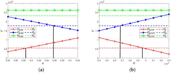
Figure 1.
Effects of two coordination factors on the profits: (a) Effects of on the profits; (b) Effects of G on the profits.
Table 4.
The optimal strategies of different models.
(1) Under the RS contract, the retailer’s expected profit improves, and the manufacturer’s profit drops with the increase of . The retailer’s expected profit becomes greater than that in the decentralized scenario once , and the manufacturer’s expected profit is higher than that in the decentralized scenario once . As a result, for achieving Pareto improvement under the RS contract, the value of ranges from (0.2877, 0.3587).
(2) Under the TPT contract, the retailer’s profit drops, and the manufacturer’s profit improves with the increase of G. The retailer’s expected profit exceeds that in the decentralized scenario once . In addition, the manufacturer’s expected profit becomes over that in the decentralized scenario once , which indicates that the Pareto improvement can be achieved under the TPT contract when G lies at (26708, 29666).
(3) The optimal emission abatement level, order quantities, and profits in the RS and TPT contracts are to be greater than those in the decentralized system, and carbon emissions are precisely the opposite. Moreover, these numerical values are consistent with those in the centralized scenario. Hence, both contracts can achieve perfect coordination. Here, the manufacturer’s highest profit is 20713, and the retailer’s highest profit is 8494. Thus, the former and the latter increase by 76.15% and 53.40% of profit at most. Nevertheless, the amount of respective profit ultimately depends on the bargaining capacity of both system members.
(4) When and G are in the range of (0.2877, 0.3587) and (26708, 29666), respectively, both the RS and TPT contracts can achieve perfect coordination and Pareto improvement. In addition, raises with the increase of . In the TPT contact, it remains constant with G, which implies that the TPT contract performed more robustly. Moreover, is higher than , which means that the TPT contract provides more advantages to the manufacturer as a leader. Hence, on this point alone, we are inclined to infer that the TPT contract is more attractive and robust.
To examine the impacts of the demand and carbon parameters, including , , , , , e, and k, on the coordinated system, the sensitivity analysis is designed by varying each parameter by , , and while keeping other parameters unchanged. A similar method can be found in Ahmed et al. (2020) [61]. When and , the overall percentage change in each variable under both contracts is summarized in Table 5.
Table 5.
Sensitivity summary with and .
Based on Table 5, we are able to come up with the following observations.
(1) The optimal order quantity is more sensitive to changes in , and the optimal wholesale prices and show higher sensitivity to movements in k under both contracts. Moreover, the optimal emission abatement level , all profits , and carbon emissions exhibit more sensitivity to movements in the parameter , which means that has the greatest impact on the economic and environmental performance. Hence, decision-makers should pay more attention to the accuracy of the stochastic demand mean information when the system achieves coordination.
(2) When each of the above seven parameters is floated up and down by 30%, the optimal emission abatement level , order quantities , supply chains’ profits , and carbon emissions behave as in the superb system, and they change by the same percentage under both the RS and TPT contracts. In addition, the optimal wholesale prices, retailers’ profits, and manufacturers’ profits have different percentage changes under both contracts, and they satisfy: , , and . This indicates that the retailer is more stable against movements in parameters under the RS contract, and the manufacturer is more stable against movements in parameters under the TPT contract. Hence, for this point, the manufacturer as a leader is more inclined to implement the TPT contract.
5.3. Managerial Insights
The research offers some managerial insights into supply chain decision making with the government’s flexible C&T policy, and the industry managers could benefit from it.
(1) The industry managers should implement an emission abatement investment, which can achieve win-win performance for both the economy and environment.
(2) Limited demand information gained by the industry managers using reliable historical data is more acceptable than the complete information.
(3) The industry managers should focus more on the accuracy of the mean information of the stochastic demand distribution because it has the greatest impact on the economic and environmental performance among seven key parameters under two coordinated contracts.
(4) Compared to the RS contract, the TPT contract performs more robustly to the manufacturer as the leader, and hence, the TPT contract is a better candidate for industry managers.
6. Conclusions
In the context of global warming, sustainable development has become a global consensus. Our research has revisited the two-echelon sustainable supply chain, considering the government, enterprise, and consumer based on a consistent goal of reducing carbon emissions. Moreover, the incomplete stochastic demand information is closer to reality. In this context, we first employ the Stackelberg game to analyze the optimal abatement and order quantity decisions that maximize the profit with complete demand information, which includes centralized and decentralized systems, respectively. Second, we formulate the distribution-free newsvendor to discuss the scenario with limited demand information, and the model also verifies the advantage of abatement investment. Furthermore, the RS and TPT contracts are explored to bridge the profit and low-carbon gap between the centralized and decentralized systems under the worst-case distribution. Numerical analyses are performed to illustrate the effectiveness of the distribution-free newsvendor model and coordination and present a sensitivity analysis of the obtained solutions. Some important findings could be derived from these observations: (1) Abatement investments are necessary to raise profits and reduce emissions. (2) The worst-case distribution is closer to the normal distribution, as compared to the uniform distribution. (3) The lower performance-cost ratio yield that limited demand information obeying the worst-case distribution is more acceptable than the complete information. (4) Under the worst distribution, both the RS and TPT contracts can achieve the centralized system‘s performance. (5) Under the worst distribution, the leader’s profit is more robust under the TPT contract compared to the RS contract in the face of variation in the coordination factor. (6) The parameter has the greatest impact on economic and environmental performance.
This research combines the distribution-free newsvendor method, game theory, contract theory, and numerical analysis to study the operation strategies and coordination optimizations with limited demand information. Several potential aspects are applicable to these theories and methods that deserve to be expanded on in future research. Future research may extend our findings by exploring the retailer-led system, where the salvage disposal or sales process generates carbon emissions and the retailer invests in abatement equipment. Another potential research topic is to consider the multi-manufacturer or multi-retailer problem in sustainable systems with limited demand information. Finally, it could be interesting to employ the distribution-free newsvendor model to study the effects of carbon emission policies on a closed-loop or dual-channel supply chain with limited demand information in different systems.
Author Contributions
Conceptualization, Y.G. and J.X.; formal analysis, Y.G. and J.X.; methodology, Y.G. and J.X.; software Y.G. and H.X.; visualization, H.X.; supervision, J.X.; writing—original draft, Y.G.; writing—review and editing, Y.G., J.X. and H.X.; funding acquisition, J.X. All authors have read and agreed to the published version of the manuscript.
Funding
This research was funded by the Innovation Project of Qufu Normal University Graduate Education, grant number QSYY16015, and the Special funds for Taishan Scholars, Shandong, grant number tsqn202103063.
Institutional Review Board Statement
Not applicable.
Informed Consent Statement
Not applicable.
Data Availability Statement
Not applicable.
Acknowledgments
We greatly appreciate the editor and the anonymous reviewers for their insightful comments and constructive suggestions, which have greatly helped us to improve the manuscript and guide us toward future research.
Conflicts of Interest
The authors declare no conflict of interest.
Appendix A. The Proof of Theorem 1
Substituting and into Equation (1), we rearrange the retailer’s profit function as and . Taking the first and second derivatives of over the order quantity q, we have:
Obviously, holds. From the first-order optimality condition, i.e., =0, we can obtain the optimal reaction function of q with the emission abatement level as . After substituting into Equation (2) and deviating the manufacturer’s profit function with regard to , we have:
It is apparent that is concave, which means that there is a unique to maximize . By solving the first-order optimality condition, we can obtain .
Appendix B. The Proof of Theorem 2
can be written as .
Firstly, we take the first and second partial derivatives of over q and obtain:
From the first-order optimality condition, we can uniquely determine that the optimal reaction function of the order quantity is .
Secondly, substituting into , the maximization problem becomes an optimization with respect to the single variable : . By taking the first and second derivatives of over , we have:
As before, assume that , it is hard to know the symbol of directly. Therefore, the third derivative of over is taken, and we have:
It can be seen that when , we have , which implies that is concave in , and vice versa is convex. Therefore, has at most three roots in the interval , which we set to , , and , satisfying .
Furthermore, we consider the following four situations to derive the optimal emission abatement level . (i) If has no root in [0,1], it means that is monotone and . (ii) If there is only one root , , it means that is concave or convex in [0,1] and .(iii) If there are two roots and , where , , and , we recover that . (iv) If there are three roots , and , then . Consequently, is one of the set .
Appendix C. The Proof of Theorem 3
Equation (A11) yields that is concave. To calculate easily, let and . Then we can acquire the optimal reaction function of the order quantity is by solving .
Substituting into Equation (7), then taking the first and second derivatives of the manufacturer’s profit , we have:
Obviously, is concave. Solving , the optimal emission abatement level is uniquely given by .
Appendix D. The Proof of Corollary 1
Substituting into and Equation (11), we easily obtain and .
Let , and from Equation (12), we have , and rearranging yields . Further, we obtain
Additionally, we easily have and ; thus, .
Appendix E. The Proof of Theorem 4
Adopting and to simplify Equation (14), and from Lemma 1, the channel’s expected profit function under the worst-case distribution is rearranged as
where .
Taking the first and second partial derivatives of over , we obtain:
From the first-order optimality condition, we obtain , where , .
Similar analysis to Theorem 2, we have:
It can be seen that when , we have , which implies that is concave in , and vice versa is convex. Therefore, has at most three roots in , which we set to , , and , satisfying . Similarly, we consider the following four situations to derive . (i) If has no root in [0,1], then . (ii) If there is only one root , , then . (iii) If there are two roots and , where , , and , then . (iv) If there are three roots , , and , then . Consequently, is one of the set .
Appendix F. The Proof of Theorem 5
Similar analysis to Theorem 3 and from the first-order optimality condition, we can obtain . Let , substituting it into and from , we can know that .
Substituting and into the profits of the retailer and manufacturer under the RS contract, we can obtain:
Appendix G. The Proof of Theorem 6
The proof is omitted because it is analogous to the Theorem 5.
References
- Sun, L.X.; Xia, Y.S.; Feng, C. Income gap and global carbon productivity inequality: A meta-frontier data envelopment analysis. Sustain. Prod. Consump. 2021, 26, 548–557. [Google Scholar] [CrossRef]
- Fan, Z.Y.; Friedmann, S.J. Low-carbon production of iron and steel: Technology options, economic assessment, and policy. Joule 2021, 5, 829–862. [Google Scholar] [CrossRef]
- Xu, J.T.; Bai, Q.G.; Xu, L.; Hu, T.T. Effects of and partial demand information on operational decisions of a newsvendor problem. J. Clean. Prod. 2018, 188, 825–839. [Google Scholar] [CrossRef]
- Wang, Z.R.; Wu, Q.H. Carbon emission reduction and product collection decisions in the closed-loop supply chain with cap-and-trade regulation. Int. J. Prod. Res. 2021, 59, 4359–4383. [Google Scholar] [CrossRef]
- Zhang, G.T.; Zhang, X.; Sun, H.; Zhao, X.Y. Three-echelon closed-loop supply chain network equilibrium under cap-and-trade regulation. Sustainaiblity 2021, 13, 6472. [Google Scholar] [CrossRef]
- Fang, Z.M.; Moolchandani, K.; Chao, H.; DeLaurentis, D. A method for emission allowances allocation in air transportation systems from a system-of-systems perspective. J. Clean. Prod. 2019, 226, 419–431. [Google Scholar] [CrossRef]
- Wang, M.; Zhao, L.D.; Herty, M. Modelling carbon trading and refrigerated logistics services within a fresh food supply chain under carbon cap-and-trade regulation. Int. J. Prod. Res. 2018, 56, 4207–4225. [Google Scholar] [CrossRef]
- Wang, S.Y.; Wu, Z.H.; Yang, B.C. Decision and performance analysis of a price-setting manufacturer with options under a flexible-cap emission trading scheme (ETS). Sustainability 2018, 10, 3681. [Google Scholar] [CrossRef] [Green Version]
- Yang, L.; Ji, J.N.; Wang, M.Z.; Wang, Z.Z. The manufacturer’s joint decisions of channel selections and carbon emission reductions under the cap-and-trade regulation. J. Clean. Prod. 2018, 193, 506–523. [Google Scholar] [CrossRef]
- Wang, S.Y.; Choi, S.H. Pareto-efficient coordination of the contract-based MTO supply chain under flexible cap-and-trade emission constraint. J. Clean. Prod. 2020, 250, 119571. [Google Scholar] [CrossRef]
- Yu, M.; Cao, E.B. Information sharing format and carbon emission abatement in a supply chain with competition. Int. J. Prod. Res. 2020, 58, 6775–6790. [Google Scholar] [CrossRef]
- Dou, G.W.; Choi, T.M. Does implementing trade-in and green technology together benefit the environment? Eur. J. Oper. Res. 2021, 295, 517–533. [Google Scholar] [CrossRef]
- Testa, F.; Nucci, B.; Iraldo, F.; Appolloni, A.; Daddi, T. Removing obstacles to the implementation of LCA among SMEs: A collective strategy for exploiting recycled wool. J. Clean. Prod. 2017, 156, 923–931. [Google Scholar] [CrossRef]
- Ma, X.L.; Xu, J.T.; Peng, W.L.; Wang, S.Y. Optimal freshness and carbon abatement decisions in a two-echelon cold chain. Appl. Math. Model. 2021, 96, 834–859. [Google Scholar] [CrossRef]
- Yang, H.X.; Chen, W.B. Retailer-driven carbon emission abatement with consumer environmental awareness and carbon tax: Revenue-sharing versus cost-sharing. Omega 2018, 78, 179–191. [Google Scholar] [CrossRef]
- Bai, Q.G.; Xu, J.T.; Zhang, Y.Z. The distributionally robust optimization model for a remanufacturing system under cap-and-trade policy: A newsvendor approach. Ann. Oper. Res. 2020. [Google Scholar] [CrossRef]
- Yadav, D.; Kumari, R.; Kumar, N.; Sarkar, B. Reduction of waste and carbon emission through the selection of items with cross-price elasticity of demand to form a sustainable supply chain with preservation technology. J. Clean. Prod. 2021, 297, 126298. [Google Scholar] [CrossRef]
- Ullah, M.; Asghar, I.; Zahid, M.; Omair, M.; AlArjani, A.; Sarkar, B. Rami fi cation of remanufacturing in a sustainable three-echelon closed-loop supply chain management for returnable products. J. Clean. Prod. 2021, 290, 125609. [Google Scholar] [CrossRef]
- Wang, M.; Zhao, L.D.; Herty, M. Joint replenishment and carbon trading in fresh food supply chains. Eur. J. Oper. Res. 2019, 277, 561–573. [Google Scholar] [CrossRef]
- Ji, T.; Xu, X.P.; Yan, X.M.; Yu, Y.G. The production decisions and cap setting with wholesale price and revenue-sharing contracts under cap-and-trade regulation. Int. J. Prod. Res. 2020, 58, 128–147. [Google Scholar] [CrossRef]
- Liu, B.Y.; Hua, Z.S.; Zhang, Q.H.; Yang, H.D.; Migdalas, A. Optimal operational decision making of manufacturers and authorized remanufacturers with patent licensing under carbon cap-and-trade regulations. Complexity 2020, 2020, 1864641. [Google Scholar]
- Bai, Q.G.; Chen, M.Y.; Xu, L. Revenue and promotional cost-sharing contract versus two-part tariff contract in coordinating sustainable supply chain systems with deteriorating items. Int. J. Prod. Econ. 2017, 187, 85–101. [Google Scholar] [CrossRef]
- Qu, S.J.; Jiang, G.Q.; Ji, Y.; Zhang, G.M.; Mohamed, N. Newsvendor’s optimal decisions under stochastic demand and cap-and-trade regulation. Environ. Dev. Sustain. 2021. [Google Scholar] [CrossRef]
- Bai, Q.G.; Meng, F.W. Impact of risk aversion on two-echelon supply chain systems with carbon constraints. J. Ind. Manag. Optim. 2020, 16, 1943–1965. [Google Scholar]
- Zheng, Y.F.; Zhou, W.H.; Chen, X.; Huang, W.X. The effect of emission permit allocation in an early-stage cap-and-trade for a duopoly market. Int. J. Prod. Res. 2020, 59, 909–925. [Google Scholar] [CrossRef]
- Chang, X.Y.; Li, Y.P.; Zhao, Y.B.; Liu, W.J.; Wu, J. Effects of carbon permits allocation methods on remanufacturing production decisions. J. Clean. Prod. 2017, 152, 281–294. [Google Scholar] [CrossRef]
- Ji, J.N.; Zhang, Z.Y.; Yang, L. Comparisons of initial carbon allowance allocation rules in an o2o retail supply chain with the cap-and-trade regulation. Int. J. Prod. Econ. 2017, 187, 68–84. [Google Scholar] [CrossRef]
- Li, L.Q.; Liu, K. Coordination contract design for the newsvendor model. Eur. J. Oper. Res. 2020, 283, 380–389. [Google Scholar] [CrossRef]
- Pasternack, B. Optimal pricing and returns policies for perishable commodities. Mark. Sci. 1985, 4, 131–132. [Google Scholar] [CrossRef]
- Hou, Y.; Wei, F.; Li, S.X.; Huang, Z.; Ashley, A. Coordination and performance analysis for a three-echelon supply chain with a revenue-sharing contract. J. Clean. Prod. 2016, 55, 202–227. [Google Scholar] [CrossRef]
- Wu, C.Q.; Li, K.P.; Shi, T.Q. Supply chain coordination with two-part tariffs under information asymmetry. J. Clean. Prod. 2017, 55, 2575–2589. [Google Scholar] [CrossRef] [Green Version]
- Shen, B.; Xu, X.Y.; Choi, T.M. Simplicity is beauty: Pricing coordination in two-product supply chains with simplest contracts under voluntary compliance. Int. J. Prod. Res. 2019, 57, 2769–2787. [Google Scholar] [CrossRef]
- He, Y.; Huang, H.F.; Li, D. Inventory and pricing decisions for a dual-channel supply chain with deteriorating products. Oper. Res. 2020, 20, 1461–1503. [Google Scholar] [CrossRef]
- Liu, W.; Zhao, H.; Song, S.J.; He, W.X.; Li, X.C. Coping with Loss Aversion and Risk Management in the Supply Chain Coordination. Sustainability 2021, 13, 4364. [Google Scholar] [CrossRef]
- Dubey, V.K.; Chavas, J.P.; Veeramani, D. Analytical framework for sustainable supply chain contract management. Int. J. Prod. Econ. 2018, 200, 240–261. [Google Scholar] [CrossRef]
- Hong, Z.F.; Guo, X.L. Green product supply chain contracts considering environmental responsibilities. Omega 2019, 83, 155–166. [Google Scholar] [CrossRef]
- Wang, Y.Y.; Yu, Z.Q.; Jin, M.Z.; Mao, J.F. Decisions and coordination of retailer-led low-carbon supply chain under altruistic preference. Eur. J. Oper. Res. 2021, 293, 910–925. [Google Scholar] [CrossRef]
- Xu, J.T.; Chen, Y.Y.; Bai, Q.G. A two-echelon sustainable supply chain coordination under cap-and-trade regulation. J. Clean. Prod. 2016, 135, 42–56. [Google Scholar] [CrossRef]
- Dong, C.W.; Shen, B.; Chow, P.S.; Yang, L.; Ng, C.T. Sustainability investment under cap-and-trade regulation. Ann. Oper. Res. 2016, 240, 509–531. [Google Scholar] [CrossRef]
- Bai, Q.G.; Gong, Y.M.; Jin, M.Z.; Xu, X.H. Effects of carbon on supply chain coordination with vendor-managed deteriorating product inventory. Int. J. Prod. Econ. 2019, 208, 83–99. [Google Scholar] [CrossRef]
- Scarf, H.; Arrow, K.J.; Karlin, S. A min-max solution of an inventory problem. Stud. Math. Theory Inventory Prod. 1958, 10, 201–209. [Google Scholar]
- Gallego, G.; Moon, I. The distribution free newsboy problem: Review and extensions. J. Oper. Res. Soc. 1993, 44, 825–834. [Google Scholar] [CrossRef]
- Mostard, J.; Koster, R.D.; Teunter, R. The distribution-free newsboy problem with resalable returns. Int. J. Prod. Econ. 2005, 97, 329–342. [Google Scholar] [CrossRef]
- Alfares, H.K.; Elmorra, H.H. The distribution-free newsboy problem: Extensions to the shortage penalty case. Int. J. Prod. Econ. 2005, 93-94, 465–477. [Google Scholar] [CrossRef]
- Lin, Y.J. Minimax distribution free procedure with backorder price discount. Int. J. Prod. Econ. 2008, 111, 118–128. [Google Scholar] [CrossRef]
- Lee, C.M.; Hsu, S.L. The effect of advertising on the distribution-free newsboy problem. Int. J. Prod. Econ. 2011, 129, 217–224. [Google Scholar] [CrossRef]
- Han, Q.M.; Du, D.L.; Zuluaga, L.F. Technical note-a risk-and ambiguity-averse extension of the max-min newsvendor order formula. Oper. Res. 2014, 62, 535–542. [Google Scholar] [CrossRef]
- Fu, Q.; Sim, C.K.; Teo, C.P. Profit sharing agreements in decentralized supply chains: A distributionally robust approach. Oper. Res. 2018, 66, 500–513. [Google Scholar] [CrossRef] [Green Version]
- Modak, N.M.; Kelle, P. Managing a dual-channel supply chain under price and delivery-time dependent stochastic demand. Eur. J. Oper. Res. 2019, 272, 147–161. [Google Scholar] [CrossRef]
- Raza, S.A.; Govindaluri, S.M. Greening and price differentiation coordination in a supply chain with partial demand information and cannibalization. J. Clean. Prod. 2019, 229, 706–726. [Google Scholar] [CrossRef]
- Fander, A.; Yaghoubi, S. Impact of fuel-efficient technology on automotive and fuel supply chain under government intervention: A case study. Appl. Math. Model. 2021, 97, 771–802. [Google Scholar] [CrossRef]
- Liu, B.Y.; Holmbom, M.; Segerstedt, A.; Chen, W.D. Effects of carbon emission regulations on remanufacturing decisions with limited information of demand distribution. Int. J. Prod. Res. 2015, 53, 532–548. [Google Scholar] [CrossRef]
- Lu, J.; Sun, X.C. Carbon regulations, production capacity, and low-carbon technology level for new products with incomplete demand information. J. Clean. Prod. 2021, 282, 124551. [Google Scholar] [CrossRef]
- Sarkis, J.; Cohen, M.J.; Dewick, P.; Schroder, P. A brave new world: Lessons from the COVID-19 pandemic for transitioning to sustainable supply and production. Resour. Conserv. Recycl. 2020, 159, 104894. [Google Scholar] [CrossRef] [PubMed]
- Leal, W.; Brandli, L.L.; Salvia, A.L.; Rayman-Bacchus, L.; Platje, J. COVID-19 and the UN Sustainable Development Goals: Threat to Solidarity or an Opportunity? Sustainability 2020, 12, 5343. [Google Scholar] [CrossRef]
- Amankwah-Amoah, J. Stepping up and stepping out of COVID-19: New challenges for environmental sustainability policies in the global airline industry. J. Clean. Prod. 2020, 271, 123000. [Google Scholar] [CrossRef]
- Ranjbari, M.; Esfandabadi, Z.S.; Zanetti, M.C.; Scagnelli, S.D.; Siebers, P.O.; Aghbashlo, M.; Peng, W.X.; Quatraro, F.; Tabatabaei, M. Three pillars of sustainability in the wake of COVID-19: A systematic review and future research agenda for sustainable development. J. Clean. Prod. 2021, 297, 126660. [Google Scholar] [CrossRef]
- Ivanov, D.; Dolgui, A. OR-methods for coping with the ripple effect in supply chains during COVID-19 pandemic: Managerial insights and research implications. Int. J. Prod. Econ. 2021. [Google Scholar] [CrossRef] [PubMed]
- Qu, Y.; Yu, Y.; Appolloni, A.; Li, M.R.; Liu, Y. Measuring Green Growth Efficiency for Chinese Manufacturing Industries. Sustainaiblity 2017, 9, 637. [Google Scholar] [CrossRef] [Green Version]
- Raza, S.A. A distribution free approach to newsvendor problem with pricing. 4OR-Q. J. Oper. Res. 2014, 12, 335–358. [Google Scholar] [CrossRef]
- Ahmed, W.; Moazzam, M.; Sarkar, B.; Rehman, S.U. Synergic effect of reworking for imperfect quality items with the integration of multi-period delay-in-payment and partial backordering in global supply chains. Engineering 2020, 7, 260–271. [Google Scholar] [CrossRef]
Publisher’s Note: MDPI stays neutral with regard to jurisdictional claims in published maps and institutional affiliations. |
© 2021 by the authors. Licensee MDPI, Basel, Switzerland. This article is an open access article distributed under the terms and conditions of the Creative Commons Attribution (CC BY) license (https://creativecommons.org/licenses/by/4.0/).