1. Introduction
In the hot arid climate that prevails in countries like Egypt, due to the long exposure of urban structures to excessive solar radiation and the Urban Heat Island (UHI) phenomenon, uncomfortable outdoor spots appear on a microclimatic scale [
1,
2]. In particular, in outdoor spots in spaces with a high building density, such as on university campuses where students spend much time undertaking their curriculum activities such as visual drawings and/or field measurements, direct and reflected radiation is more absorbed, and more anthropogenic heat is released, [
3] putting users under higher thermal stress. To alleviate the impact of the UHI phenomenon on the health and well-being of the occupants of these outdoor spaces, investigating and manipulating the impact of urban built environment elements such as the arrangement of buildings, the orientation of open spaces, the aspect ratio, and shaded areas on the thermal comfort performance of these spots become crucial in the early stages of the design process either on the urban or architecture scale [
4].
Urban geometry and vegetation are the most influential factors in an open space’s microclimate [
5,
6]. Urban open spaces’ geometry, which is formed by building density, height, and orientation, differentiates one urban canyon from another, causing a different impact on microclimate, mostly through trapping heat. The relevant attributes that often cause differences in urban geometry are the Height/Width ratio (H/W) and the Sky View Factor (SVF) [
5].
Owing to the significant role of SVF in describing the complexity and interventions of urban form elements [
7], several studies have addressed this to investigate the impact of the shading effect on microclimate in various urban patterns [
8] and various climatic zones [
9,
10,
11]. SVF is defined as the ratio of radiation received from the sky by a planar surface to that received from the entire hemispheric radiating environment [
12]. It is a numerical dimensionless value between 0 and 1. An SVF of 0 is a completely enclosed environment, and an SVF of 1 is a completely open area without any obstructive elements.
The influence of SVF coupled with the aspect ratio (H/W) on meteorological parameters and outdoor thermal comfort has been commonly studied in the context of street canyons, which are considered to have a simplified rectangular vertical profile with an infinite length. It has been found that in the hot season in cities in cold deserts, such as Isfahan in Iran, the impact of SVF in four streets with different H/Ws and different amounts and arrangements of greenery on microclimatic variables varied with the street orientation. Moreover, the variation in the air temperature was the smallest, whereas the impact was most significant, on mean radiant temperature (T
mrt) and surface temperature. Additionally, there was a significant and positive relation between SVF and Physiological Equivalent Temperature (PET) [
13].
Contrarily, in high-rise urban residential environments in Tehran, Iran [
14], it was found that during the hottest and the coldest days in the year, there was a direct relation between SVF and air temperature during the day and an inverse relation at night. In the temperate oceanic climatic region, such as southern Brazil, which has dry winter seasons [
10], it was found that the variation in T
mrt was closely related to the variation in SVF. However, their results suggested that, during the daytime, the impact of other climatic variables and urban features makes SVF not the main determinant of outdoor thermal comfort. A smaller SVF showed a lower range of thermal sensation, while with a higher SVF, the thermal sensation was more dispersed in the outdoor environment in commercial pedestrian streets in severely cold regions of China [
15]. The latter results are compatible with [
7], who investigated the relation between SVF and microclimatic values in nine local climate zone models by applying the typical summer meteorological conditions of Nanjing, China. It has been found that SVF as an indicator of building heights, layouts, and densities is correlated with the predicted mean vote (PMV) and T
mrt. Meanwhile, [
16] stated that, generally, expanded SVF retained less warm air and reduced absorbed radiation.
Further, through the investigation of urban open spaces such as university campuses [
17], it was found that in the tropical climate of Taiwan, students experienced discomfort in hot summer in barely shaded areas with high SVF values as well as in mild winter in highly shaded areas with lower SVF values. Therefore, the researchers recommended that the designers provide sufficient shading by trees and buildings in the summer without creating excessive shadowed areas because low temperatures also caused discomfort in Taiwan.
In a subtropical climate, a higher SVF during daytime created an extreme outdoor environment in campus clusters due to the environment’s radiation. Furthermore, there was a significant effect of SVF on air temperature [
18]. Moreover, the studies mentioned above show that the effect of SVF on microclimatic conditions and thermal comfort has been most studied in street canyons, but very few studies have been conducted on universities, particularly those in hot arid climates. Such an effect even varied from location to location in the same climatic context due to the variance of urban space geometrical parameters, such as aspect ratio (H/W) and length to width (L/W) [
19], and the dynamic interactions between microclimatic variables in open spaces.
In Assiut University, which is located in a hot arid region in southern Egypt, an evaluation of different shading strategies in different locations [
20] showed that air temperature degrees increased in the sitting areas where SVF values were high due to the low density of trees and the low value of H/W. Further, they found that increasing the density of trees in the main open space caused a reduction of 0.7 °C in the average temperature and the predicted mean vote (PMV), leading to a more comfortable space for the students. Urban trees have proved to have a cooling effect in hot times of various climatic regions, which is related to the tree geometry, foliage density, evapotranspiration, and trees’ planting patterns and contributes to modifying its near microclimate conditions—basically, its canopies control SVF, hence modifying the site incident solar radiation [
21,
22,
23,
24]. However, studying urban trees’ microclimate in university campuses is much differentiated from in street canyons, as campuses may include different, irregular urban spaces with different occupation time schedules owing to their differentiated activities. The architecture engineering department plaza, Cairo University, and Assiut University, Egypt, are examples of this [
20]. The former example is a plaza in a high building density area, surrounded by the engineering faculty’s multi-story buildings, whose layout geometries are difficult to adjust after the many years of construction. Up to 80 students use the plaza at a time, and the only way to provide shelter for them from excessive solar radiation is to adjust their SVF and mitigate the heat stress. This is why it was crucial to assess the microclimate of trees in the site and to address the correlation of SVF that those trees contribute to with thermal comfort to extract implications.
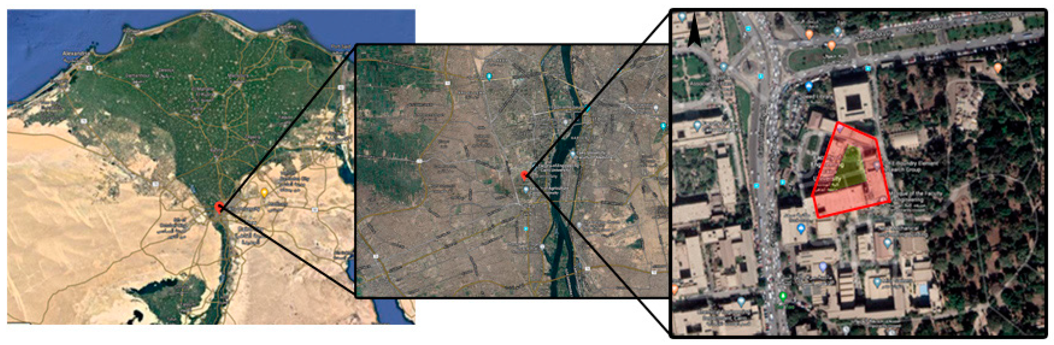
Figure 1 indicates the research case study location, architecture engineering department plaza of Cairo University, Giza, Egypt, which is located at 30.0131° N, 31.2089° E. Giza has a hot, arid climate and falls in the “hot desert climate” type according to the Köppen climate classification [
25]. Giza receives a significant amount of solar radiation throughout the year. The average hourly maximum solar radiation exceeds 6 kWh/m
2/d for almost 50% of the year [
26].
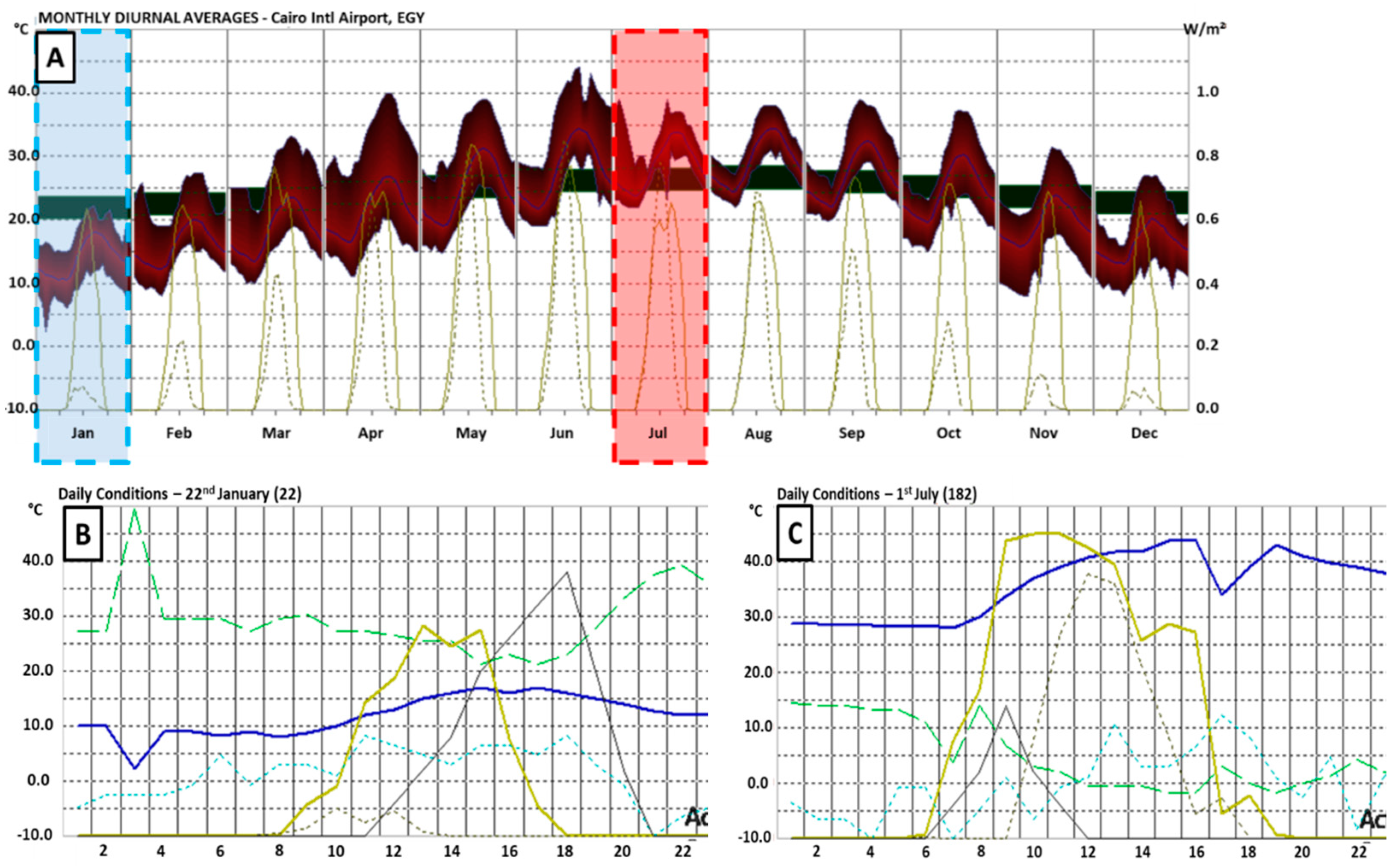
Ecotect weather analysis program was used to identify the two days that had the average temperature of each of the two seasons.
Figure 2 Ecotect shows that the temperature on the 22nd of January matched the average temperature for the cold season and that on 1st July matched the average for the hot season.
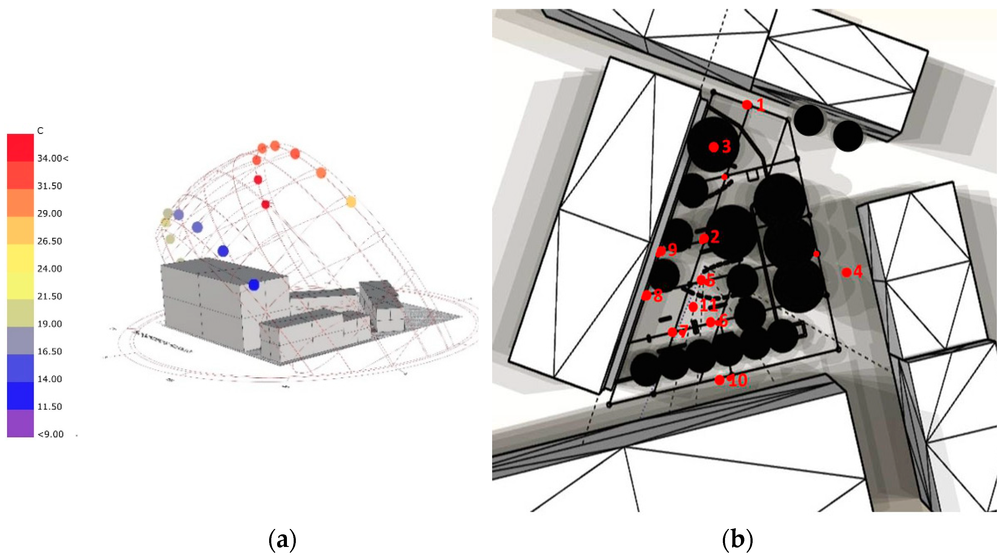
1.1. Urban Geometry Characteristics
The grid of the eighteenth points
Figure 3 comprises different urban geometry features and provides a variety of shading levels (e.g., under the trees’ crowns, near buildings, and in the un-shaded areas). Three sides of the semi-enclosed open space are surrounded by three streets (
Table 1):
Street 1 is a 6 m wide and WNW–ESE-oriented street. Four points were assigned in the middle of this street (1, 2, 3, and 4).
Street 2 is a 6 m wide NNW–SSE oriented street from which four points were selected: three points (9, 10, and 14) near three trees—one near a large, old Cassia leptophylla tree and two near mature Cassia nodosa tree—and the last point (number 15) at the end of the street.
Street 3 is a 6 m wide ENE–WSW-oriented street. Three points on it (16, 17, and 18) were selected.
Zone 1 is a semi-enclosed open space, surrounded by the three streets mentioned above and one building, and two points (6 and 7) 1.5 m away from the building, to avoid long wave reflection and emission, were selected. Point (8) was directly under the canopy of a large old Cassia leptophylla tree. Five points (5, 8, 11, 12, and 13) were located in the middle of the open space in the sunny spots in the middle of the seating zone.
The finishing material of the seating area where seven points are located is yellow cement blocks, the albedo of which is 0.5, whereas the albedo of the asphalt of the surrounding streets is 0.2. Eleven points are located on these streets.
1.2. Vegetation Characteristics
Two types of the most common Egyptian urban environment trees are on the site. They are the deciduous/semi-deciduous
C. nodosa and the semi-evergreen
C. leptophylla. These trees’ physical characteristics, such as leaf area density (LAD) and the albedo values for each type at different heights, were adopted from [
27].
Table 2 shows the simulation setup for the use of Leaf Area Index (LAI)-2000 (plant canopy analyzer instrument) [
28].
3. Results
Microclimatic variables were analyzed for eight hours from 09:00 to 17:00 while the selected space was occupied. The minimum value of air temperature was at point 17 at 09:00 LST in the hot season, and the mean radiant temperature was at its minimum at point 4 at 17:00 LST. The air temperature was at its maximum at point 11 at 13:00 LST, and the mean radiant temperature was at its maximum at point 8 at 14:00 LST. On the other hand, the minimum relative humidity was at point 11 at 13:00 LST, and the maximum was at 09:00 LST at point 13. The highest wind speed was recorded at point 18 at 17:00 LST, whereas the lowest wind speed was recorded at point 6 at 09:00LST. For each Ta, Tmrt, RH, and V, the values ranged between 28.85 and 34.1 °C, 30.83 and 75.4 °C, 37.2% and 53.1%, and 0.18 and 2.6 m/s, respectively.
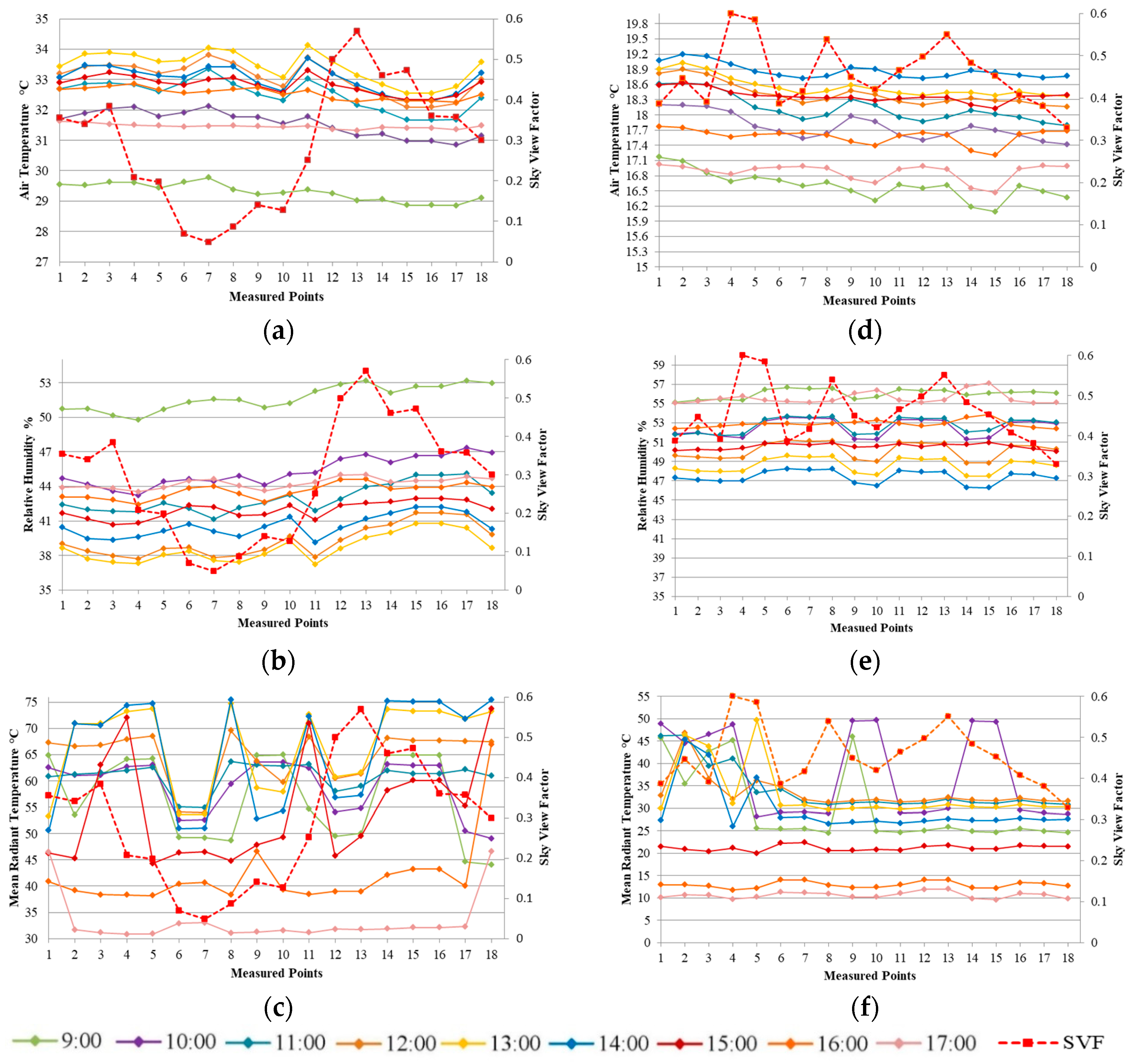
As shown in
Figure 8a, throughout the simulation hours, the air temperature was increasing at all the 18 points before it declined noticeably after 13:00 LST, and they became roughly convergent at 17:00 LST. From 09:00 to 12:00 LST, T
a was the highest at point 7. However, from 13:00 to 15:00 LST, the air temperature at point 11 remained the highest and higher by 1 °C than at point 13, where the highest SVF was found. The lowest values were revealed in street 3, where values were lower by 0.1–1.3 °C than points in street 1—however, the temperature increased as they approached point 18. Moving from point 4 towards point 15, the Ta values decreased gradually toward the south–east along street 2. Overall, at most hours, peaks were observed at point 11 followed by point 7 and the points in street 1, while the minimum levels were observed in street 3.
In contrast with the Ta values, the highest values of RH (
Figure 8b) for all points were at 09:00 LST and decreased at all the points before increasing at 13:00 LST, except at Point 11, which remained at the lowest values from 11:00 to 15:00 LST before it increased after 15:00 LST. The RH values at the points on street 3 were higher than at the points on street 1. However, they decreased towards point 18. In general, in the simulation, the difference between relative values for all points diminished as 17:00 LST approached.
In the simulation, the mean radiant temperature values at all hours and all points fluctuated as shown in
Figure 8c, whereas from 09:00 to 14:00 LST, values at points 6, 7, and 8 were at their lowest values in comparison with the other points before they rose higher than others starting from 15:00 LST. Particularly at point 18, the T
mrt was higher by 18 °C than at point 17. At point 8, where SVF was low at 0.08, the T
mrt was nearly equal to the T
mrt at points 6 and 7 at 09:00 LST. After that, the T
mrt at point 8 increased and peaked at 14:00 LST, when it was higher than at points 6 and 7 by 24 °C. Thereafter, it decreased steeply by 30 °C to a level lower than at points 6 and 7. Like the T
mrt values at point 8, T
mrt at point 11 began rising and exceeded T
mrt at other points and peaked at 15:00 LST to exceed that at points 6 and 7 by 22 °C, a level of excess just less than that reached by the T
mrt at point 8. Thereafter, it decreased noticeably to become lower than the T
mrt at points 6 and 7. At point 8, it was lower by 31 °C than at point 13, where the highest average values of SVF and T
mrt were observed throughout the simulation. They reached their peak, 61.5 °C, at 13:00 LST. However, it was low in comparison with the values in street 1 and street 3. Generally, peaks at most of the hours were detected in streets 1 and 3, while minimum values were observed at the shaded points 6 and 7 in zone.
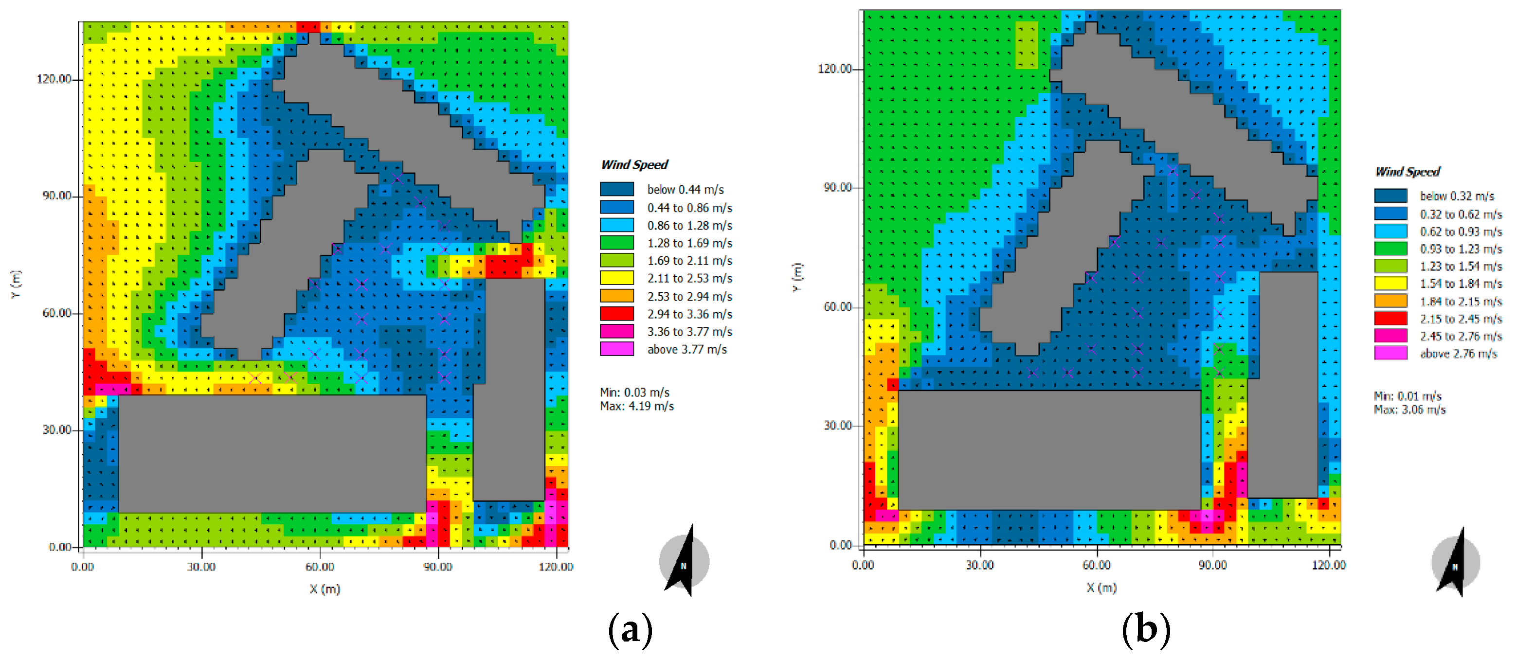
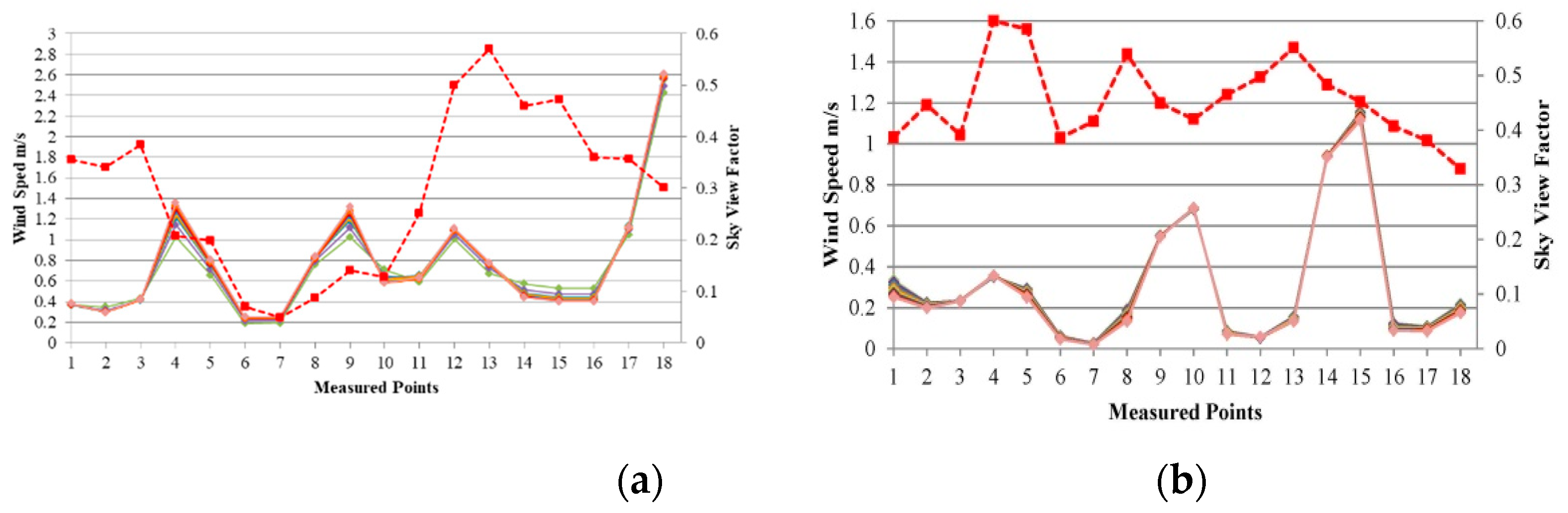
The prevailing wind direction was northeasterly
Figure 9a. Wind speed in
Figure 10a was almost steady at 0.18–2.6 m/s during all hours and at all points in the simulation. The values had an ascending trend from point 1 to point 4. It was lower at points in zone 1, particularly at points 6 and 7, where the lowest values were observed at 09:00 LST. The speed increased towards point 9. However, it decreased as one headed toward the south. On the contrary, the highest values were found in street 3, where it increased from point 16 and peaked at point 18. At the points in the middle of zone 1, such as points 5, 8, 11, and 12, the average values of V were higher by 0.4 to 0.6 m/s than at the points close to the building, such as points 6 and 7; however, V showed an ascending trend toward the south from point 5 toward point 12, where the V values were high throughout all hours in the simulation. In general, the lowest values were at points in street 1 as compared to street 2, while, in contrast, the highest values were at points in street 3.
In the cold season, the air temperature values ranged between 16.00 and 19.2 °C. As shown in
Figure 8e, air temperature values at points in street 1 increased noticeably from 09:00 to 14:00 LST throughout all the simulated hours, and the highest value was observed at point 2 at 14:00 LST. At this hour, T
a was 18.9 °C at points 9 and 10 in street 2. These were among the highest values after point 2, while the lowest value was found at point 15 at 09:00 LST, followed by point 14. However, their T
a increased by 2.4 °C at 14:00 LST. T
a at points 6, 7, and 8 also increased as afternoon approached. However, the increase was between 0.1 and 0.4 °C, which was a lesser rate than that at the points in streets 1 and 2. Street 3’s values were among the lowest as compared to those in streets 1 and 2. A noticeable decrease of 0.7 °C at points 14 and 15 occurred at 15:00 LST. Generally, in all the simulation hours, the highest temperature values were recorded in street 1, whereas the lowest values were recorded in street 3.
The relative humidity values in
Figure 8f ranged between 46.2% and 57.1%, and the highest values were at 09:00 LST and 17:00 LST, while the lowest values were at 14:00 LST with a reduction between 0.5% and 1.39% during the simulation. Both minimum and maximum values were recorded at point 15 followed by point 14 at 14:00 and 17:00 LST, respectively. Points in zone 1 and street 3 had a difference of 1%–2% higher than other points from 10:00 to 13:00 LST. A noticeable increment of 6% was at points in street 2 from 15:00 till 17:00 LST. Overall, at almost all simulation hours, the highest RH values were at points in zone 1 and street 3 compared to street 1 and street 2.
The mean radiant temperature in
Figure 8g ranged between 9.06 and 49.60 °C, since the lowest T
mrt was at p15 at 17:00 LST while the highest value was at p5 at 13:00 LST. Points in street 1 showed high values of T
mrt in the forenoon, particularly at point 2, where values were high until 14:00 LST, when it noticeably decreased by 24.4 °C. Points in zone 1 remained roughly increasing by 2–4 °C until 13:00 LST, and then it began decreasing, except for point 5, where the highest value was revealed by an obvious increase of 13 °C from 12:00 LST to 13:00 LST before it decreased 12.8 °C at 14:00 LST. Point 10, point 14, and point 15 showed a noticeable increase of 25 °C from 09:00 to 10:00 LST; point 9 T
mrt was high at 09:00 and 10:00 LST, then it lowered to 18 °C at 11:00 LST. In general, values at points in street 1 were high in comparison to street 3 and zone 1 until 14:00 LST, followed by points 9 and 10 at street 2, which were high until 11:00 LST, relative to the other points.
As expected, the prevailing wind direction was blocked by surrounding buildings, reducing the release of trapped heat and RH. As shown in
Figure 9, the prevailing wind direction was northwest, and wind speed in
Figure 10b was unvaried through all the simulation hours at each point and ranged between 0.01 and 1.15 m/s. The highest values were found at point 15, followed by point 14, where V was 0.9 m/s, followed by point 10, where V was 0.6 m/s, and further followed by point 9, where V was 0.5 m/s. The lowest values were found at zone 1 at point 7 and point 6, followed by point 12 and point 11, where V was 0.05 and 0.08 m/s, respectively. Points in street 3 also demonstrated low values of V; however, their values were slightly higher before the afternoon. Moreover, V was higher by 0.1 m/s at point 18. Overall, all the highest values of V were observed in street 2 at point 15 and decreased as one moved northward. These were followed by values at points in street 1. The lowest values were in zone 1, particularly at points nearer to the 12 m high administrative building, such as at point 12, and it decreased gradually from points in the south, such as point 13, where V was 0.15 m/s, towards points located in the north until it was lowest at point 7 followed by point 6. Additionally, values at points in street 3, particularly at point 18, were higher than points in zone 1.
3.1. SVF, Microclimatic Variables and Thermal Comfort
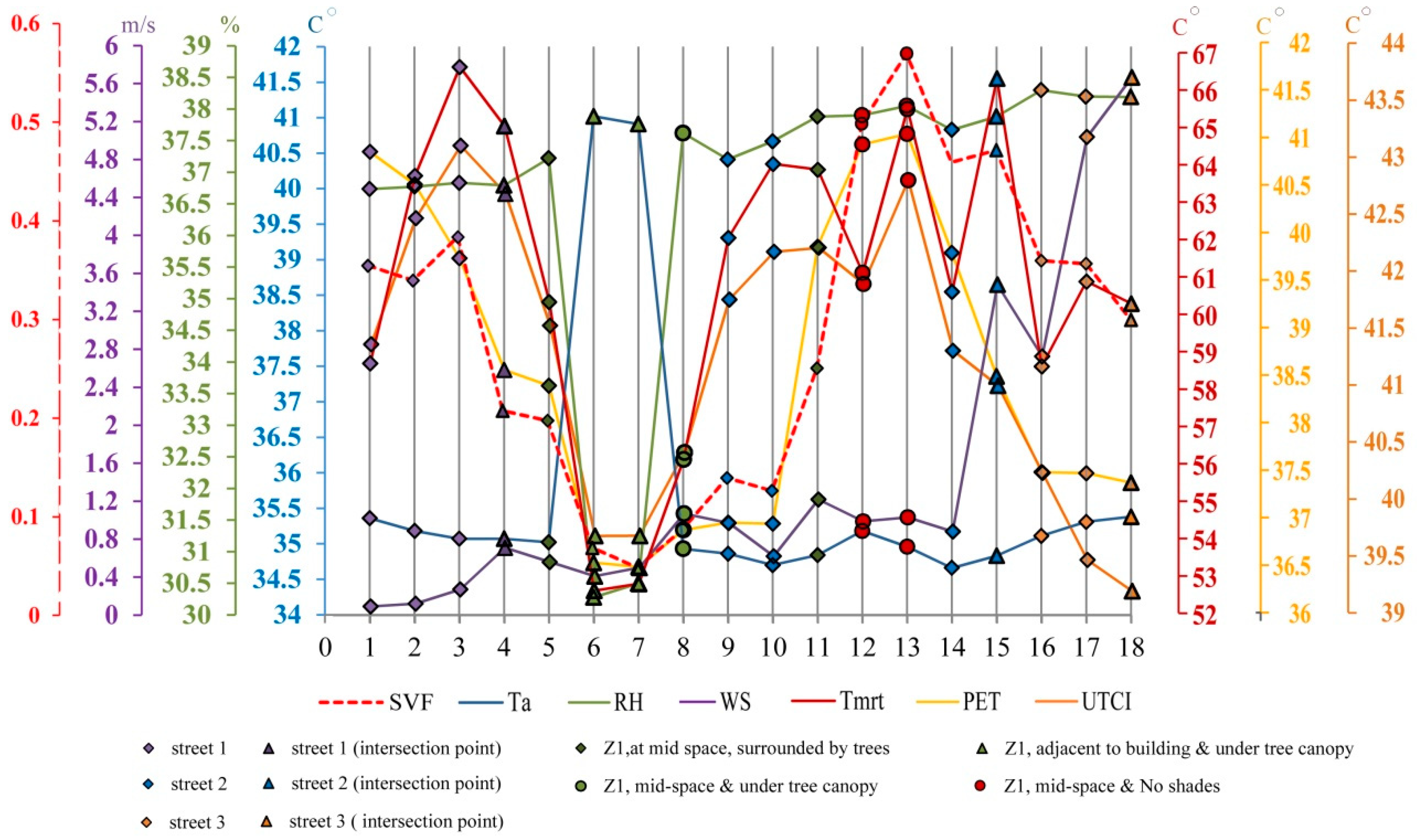
As shown in
Figure 11 and
Figure 12, the 18 points were categorized according to their location in the open space, describing the surrounding urban features from
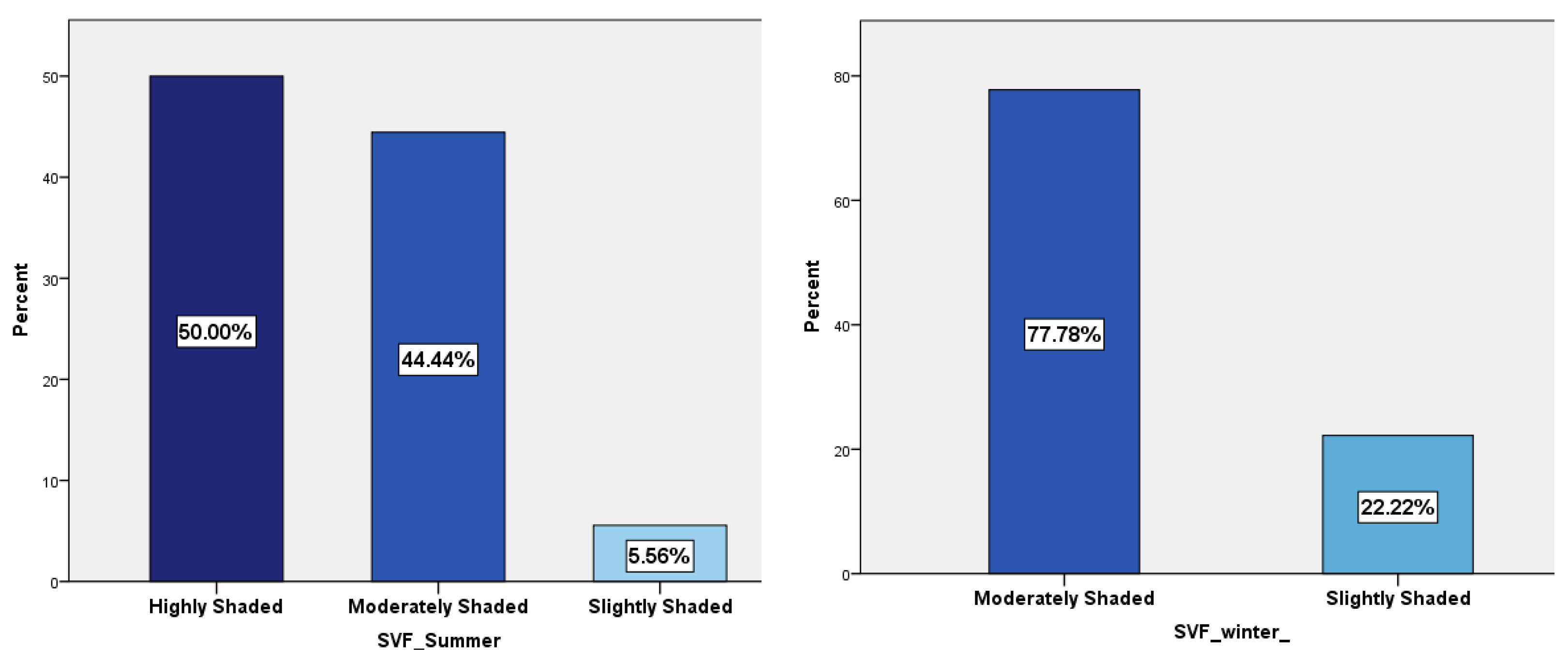
Table 1. In the summer (
Figure 11), SVF ranged from 0.04 to 0.5, and the average air temperature T
a_
avg ranged from 31.6 to 32.6 °C. The highest value was found at point 7 despite the lowest SVF value of 0.049 that it had. They were followed by point 11, where the T
a_
avg was 32.6 °C. Points in street 1 showed high values of T
a_
avg between 32.3 and 32.5 °C compared to street 3, where the lowest value, 31.6 °C, was found. However, there was a slight increase of 0.5 °C at point 18. T
a_
avg values were 32.3 °C at point 5 and point 6 increased by 0.1 °C at point 8. The highest SVF value was observed at point 13, followed by point 12; these points showed low values of T
a_
avg at 31.9 °C and 32.1 °C, respectively.
The average relative humidity, RH_avg, highest values were found at the points in street 3 since the highest value was 44.6% at point 17 followed by point 16 and point 15, while it decreased 1% at point 18. The lowest values were found at street 1 at point 4, where RH_avg was 41.8%, and it increased gradually towards point 1 where the value was 42.7%. A slight difference of 0.1% was observed among points located in zone 1 where values were between 42.4% and 42.9%; a slight rise of 1.5% at point 12 and point 13 was also observed. In street 2, values continued to increase, starting from point 9 (42.5%) towards point 14 (43.95%).
Concerning Tmrt, the highest average value was 62 °C observed at point 18 despite its location in the deep canyon. Moreover, it had the highest value of an average wind speed of 2.5 m/s. On the other hand, it was found that the lowest value of Tmrt_avg was 48.4 °C at point 6, which also demonstrated the lowest value of wind speed, 0.2 m/s. At points in street 1, these values increased towards point 4 to reach 60.6 °C and 1.2 m/s with a difference of 6 °C and 0.9 m/s from point 1, respectively.
In terms of outdoor thermal comfort indices, PET average values ranged from 36.8 to 41.07 °C, while UTCI ranged from 28.4 to 31.6 °C. PET and UTCI showed their lowest average values at both points 7 and 6, which were 36.8 °C and 28.4 °C, respectively, whereas the lowest values of SVF were also seen. The highest value of PET_
avg was at point 13, followed by point 12, where the highest values of SVF also was recorded, while the highest value of UTCI_
avg was 31.62 °C at point 4. All points were considered to be uncomfortable for PET values since the thermal comfort ranged 23–32 °C [
44]. Meanwhile, regarding UTCI values, according to the UTCI assessment scale [
36], all points indicated moderate heat stress, even the lowest values.
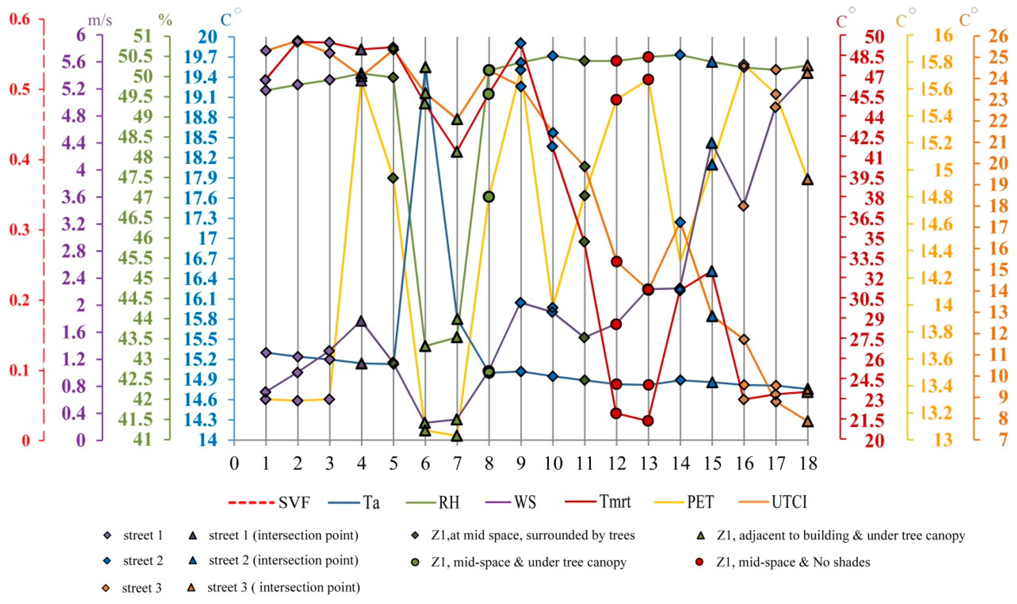
In the cold season, SVF values ranged 0.3–0.6 and T
a_
avg ranged from 17.6 to 18.2 °C (
Figure 12). Point 2, with an SVF of 0.4, showed the highest value of T
a_
avg and T
mrt_
avg and UTCI, which were 34.3 and −0.35 °C, respectively. The lowest value of T
a_
avg was demonstrated at point 15, accompanied by the highest value of V_
avg 1.1 m/s. T
a_
avg values in street 1 were the highest in comparison to street 2 and 3. T
a_
avg under tree canopy in zone 1 at point 8 was 17.8 °C, where the lowest value of T
mrt_
avg was 24 °C. On the other hand, the minimum value of RH_
avg was 51.2% at point 3 with SVF = 0.39; the maximum value was 52.4% at point 6, where SVF equals 0.3. Point 7 showed the lowest V_
avg 0.02 m/s as it showed the lowest value of PET_
avg 13 °C. The highest value of PET was 15.78 °C found at point 16, although T
a_
avg was 17.8 °C. The lowest value of the UTCI value was −4.4 °C at point 18, where the lowest SVF value, 0.32, was found.
3.2. Correlation between SVF, Microclimatic Variables, and Thermal Comfort
Finally, at the statistical analysis phase, the correlation between SVF and the average values of the microclimatic variables, PET and UTCI, which are required to express the central tendency of the results during the whole period of occupation at each point, was analyzed throughout the daytime during both seasons, with the average values of each variable indicated by Ta_avg, Tmrt_avg, RH_avg, V_avg, PET_avg, and UTCI_avg.
Table 7 shows Pearson’s bivariate test (r) to explore the strength and type of correlation between variables considering the significance level and r coefficient interpretation, since there is no correlation when r = 0, it is weak when 0 < r < 0.25, it is moderate when 0.25 < r < 0.75, and it is strong when r > 0.75 [
45]. In the summer, the test showed a moderate correlation between SVF and T
a, T
mrt, RH, PET, and UTCI as r = −0.57, r = 0.71, r = 0.51, r = 0.68, and r = 0.53, respectively. On the other hand, the correlation of V with SVF was not at a significant level. In the winter, SVF showed no correlation with any microclimatic variables, even PET and UTCI.
Table 8 illustrates the correlation between SVF and the microclimatic variables, PET and UTCI, which showed a correlated linear variation significantly in the Pearson test for the two seasons. Regarding SVF and Ta_
avg Equation (1), the intercept a = 32.52 implies that T
a_
avg at a completely shaded point with no sun penetration was 32.52 °C. Furthermore, the slope b = −1.15 expresses that T
a_
avg decreased 0.1 °C per 0.1 unit increase in SVF, which indicates the lesser the shade at any point, the lesser will be the average air temperature.
At Tmrt_avg Equation (2), the slope b = 25.63 is equivalent to an increase in Tmrt_avg value by 2.5 °C per 0.1 unit of SVF, which indicates the lesser shade at any point, the more mean radiant temperature the occupants experience at this point. Tmrt at a completely shaded area equals 49.9 °C, while RH showed a positive correlation with SVF since it increased 0.3% per each 0.1 unit increase in SVF RH_avg Equation (3). Moreover, it equals 42.2% at a completely shaded point. In SVF and PET_avg Equation (4), intercept a = 36.3 °C (uncomfortable) determined that PET was 36.3 °C at a completely shaded point, and it increased 0.4 °C per 0.1 unit increase in SVF according to the slope (b = 7.92). UTCI_avg Equation (5) showed a lower value (28.61 °C) at the completely shaded point, and it increased by 2.5 °C at each 0.1 unit increase in SVF.


