Article

Assessing and Predicting the Impact of Multi-Scenario Land Use Changes on the Ecosystem Service Value: A Case Study in the Upstream of Xiong’an New Area, China

1
Key Laboratory of Agricultural Water Resources, Center for Agricultural Resources Research, Institute of Genetics and Developmental Biology, Chinese Academy of Sciences, Shijiazhuang 050021, China
2
College of Advanced Agricultural Sciences, University of Chinese Academy of Sciences, Beijing 100049, China
*
Author to whom correspondence should be addressed.
Sustainability 2021, 13(2), 704; https://doi.org/10.3390/su13020704
Submission received: 3 December 2020 / Revised: 28 December 2020 / Accepted: 8 January 2021 / Published: 13 January 2021
(This article belongs to the Special Issue Environmental Impact Assessment and the Culture of Sustainability)

Abstract

:
The evaluation of ecosystem service value has become the basis of ecological protection, ecological regionalization, and ecological compensations. Land use changes have taken place due to several natural and anthropogenic reasons, significantly influencing the ecosystem services value (ESV). In this study, we used an interactive coupling model that simulates future land use changes and the equivalent coefficient table method to predict and evaluate the ecosystem service value in the upstream of Xiong’an New Area in 2035, and we quantitatively calculated the impact of land use changes on the ecosystem service value under four future scenarios. The results indicate that from 2015 to 2035, the ecosystem service value in the production scenario and life scenario decreased significantly by CNY 1635.39 million and 561.95 million, respectively, and the areas where the ESV decreased mainly appeared in river banks and surrounding areas of towns. The conversion of forest land to cultivated land and the conversion of grassland to construction land are the main reasons for the reduction of the ecosystem service value in the production scenario and life scenario, respectively. The ecosystem service value in the ecological scenario increased significantly by CNY 2550.59 million, and the conversion of grassland to waters is the main reason for the increase in ecosystem service value, with a contribution rate of 73.89%. Moreover, due to the trade-off between ecosystem services, the overall change of ecosystem service value in the current scenario is not obvious. In conclusion, strictly controlling the scale of construction land, strengthening the management and protection of water resources, and expanding the afforestation scale may improve the ecosystem service value of the upstream Xiong’an New Area in the future.

1. Introduction

Ecosystem services refer to life support products and services obtained directly or indirectly through the ecosystem’s structure, processes, and functions, including provisioning services, regulating services, supporting services, and cultural services [1,2]. The sustainable development of the social economy depends on the sustainable supply of ecosystem services. However, rapid population growth, coupled with economic growth and global climate change, are producing various environmental problems, which severely threaten the ability of ecosystems to provide ecosystem services [3,4]. Quantifying, valuing, and mapping ecosystem services are becoming important and reliable tools for ecological environment management and policy making [5,6]. Costanza et al. used the “willingness to pay” method to evaluate the global ecosystem service value (ESV) [7], which provides new methods and ideas for the study of ESV. Based on the research of Costanza et al., Xie et al. constructed a method for valuing ecosystem services based on expert knowledge [8], and it has been widely used in the evaluation of ESV at sample, regional, and national scales [9,10].
Land use change alters the physical parameters of the earth’s surface, modifies the ecosystem productivity, influences nutritional provision from soil to vegetation by changing biochemical cycles, and significantly affects ecosystem services ranging from water supply to biodiversity [11,12,13]. In the past few decades, human-dominated land use change (e.g., forest overexploitation, agricultural intensification, and urbanization) has changed ecosystems more drastically and extensively than ever before, leading to substantial and largely irreversible loss of ecosystem services [14,15,16]. Diaz et al. noted that the land use change from natural land to urban and cultivated land has accelerated the loss of biodiversity, leading to a decrease in the ecosystem’s stability [17]. Deng et al. found that the increase in land use intensity and the resulting change in vegetation cover can significantly change hydrological processes, including the cycle of chemical elements, thereby affecting hydrological ecosystem services [18]. Cultivated land is an essential part of a country’s ecological environment because it is one of the most important provisioning services in the ecosystem [19]. However, land use changes caused by rapid urbanization have reduced the quality and quantity of cultivated land, which has reduced the food provisioning services provided by agricultural ecosystems [20]. Song et al. assessed the impacts of land use change on the ESV in the rapidly urbanizing North China Plains and found that the conversion from cultivated land to construction land decreased the ESV by 66.5% [21]. Moreover, many previous studies have found that climatic factors (e.g., precipitation and temperature variations) have long-term effects that alter the natural landscape dynamics and significantly impact specific ecosystem services, such as carbon sequestration and raw material production [22,23].
Land use change is a complex process intertwined with nature and economic activities. On the one hand, the land’s natural material conditions provide the possibility and suitability of land use [24]. On the other hand, the final use range, structure, and method of land depend on the rationality and feasibility of socioeconomic and technological innovation, and are deeply affected by the level of urban and rural industrial development and industrial structure [25,26]. With the continuous changes in national policies, social needs and the natural environment, the types and structures of land use will inevitably change. Although the government has made strong interventions in land use planning, future land use changes cannot be accurately forecasted [27]. In view of the complexity and uncertainty of future land use changes, land use change simulation models need to be used to evaluate the impact of land use changes on ESV under different scenarios. Xu et al. suggested these models should be either “top down” or “bottom up” [28]. The “top-down” model, such as the system dynamics (SD) model, focuses on the relationship between different land use types at the macro level and is usually used to predict the magnitude of land use change [29]. However, the “top-down” model cannot predict the spatial pattern of land use [30]. In contrast, the “bottom-up” model predicts land use changes in all grid cells by establishing a regular grid, and it can predict the spatial pattern of land use [31]. One widely used “bottom-up” model is the future land use simulation (FLUS) model, which can effectively deal with the complexity and uncertainty of converting various land use types under the mutual influence of the human–land relationship [32]. Some studies have coupled “top-down” and “bottom-up” approaches. In this coupling, the “top-down” method is used to determine the amount of future land use change. Subsequently, a “bottom-up” approach is used to allocate these land-use changes on grid cells [33,34]. However, current the coupled model directly integrate two models via land use demands at the end of the study period, while the interaction and feedback between the two models are ignored [30,35]. Moreover, the spatially explicit allocation of land use change to a grid cell involves a complex process that must identify the relationships between land use change and its driving forces [36]. The impact of human activities on climate change is increasing; thus, if climate change scenarios are not taken into account, these models are not suitable for the simulation of land use changes under human-climate-included scenarios [37].
In this paper, we interactively integrate the “top-down” SD and the “bottom-up” FLUS model to simulate and predict future land use changes in multiple scenarios. In the coupled model, we incorporate natural factors (including future climate variations and socioeconomic development) into the SD and FLUS models. In addition, driving force factors of different degrees were set in the SD model according to the future scenarios designed, and different internal conversion costs were set in the FLUS model accordingly, so as to meet the actual characteristics of land use change and conversion under different scenarios. We present a case study in the upstream of Xiong’an New Area to investigate how land use changes under different scenarios in 2025 will affect the ESV by applying the coupling model. The aims of this paper are (1) the simulation and prediction of land use changes under different scenarios in the upstream of Xiong’an New Area; (2) the evaluation of changes in ESV under different land use change scenarios; and (3) the calculation of the contribution rate of land use change to the ESV under four future scenarios.

2. Materials and Methods

2.1. Overview of the Study Area

The study area includes three basins in the upstream of Xiong’an New Area, across Hebei and Shanxi provinces of the Northern China, Zijingguan, Zhongtangmei and Fuping basins, with a total area of 7310.27 km2 (Figure 1) [38]. The terrain of the study area is high in the northwest and low in the southeast, with an average altitude of 1108 m and an average slope of about 19°, which belongs to the mountain–plain interlaced area with frequent human activities [39]. The study area has a monsoon climate of the medium latitudes zone with an average annual temperature of 7.4 to 12.8 °C and annual precipitation of 550 to 790 mm. Affected by the monsoon climate, precipitation in the study area was uneven throughout the year; nearly 80% was concentrated from June to September [40].
On 1 April 2017, China’s Central Committee and State Council decided to establish the Xiong’an New Area. The upstream of Xiong’an New Area is an important ecological environment support area and water conservation function area. The change in ecosystem services in this area will directly affect the ecology, water supply, and flood control safety of Xiong’an New Area [38]. However, with the increase in global warming and human disturbance, the land use in this area has changed significantly, and the ecological environment is facing unprecedented pressure [41]. The recent joint statement from China’s the Central Committee and State Council passed the “Hebei Xiong’an New Area Master Plan (2018–2035)”, which describes the plans to build the New Area into a green, ecological, and livable new city by 2035 [42]. This puts forward higher requirements for protecting and improving the ecological environment in the upstream of Xiong’an New Area in the future.

2.2. Land Use Change Multi-Scenario Simulation

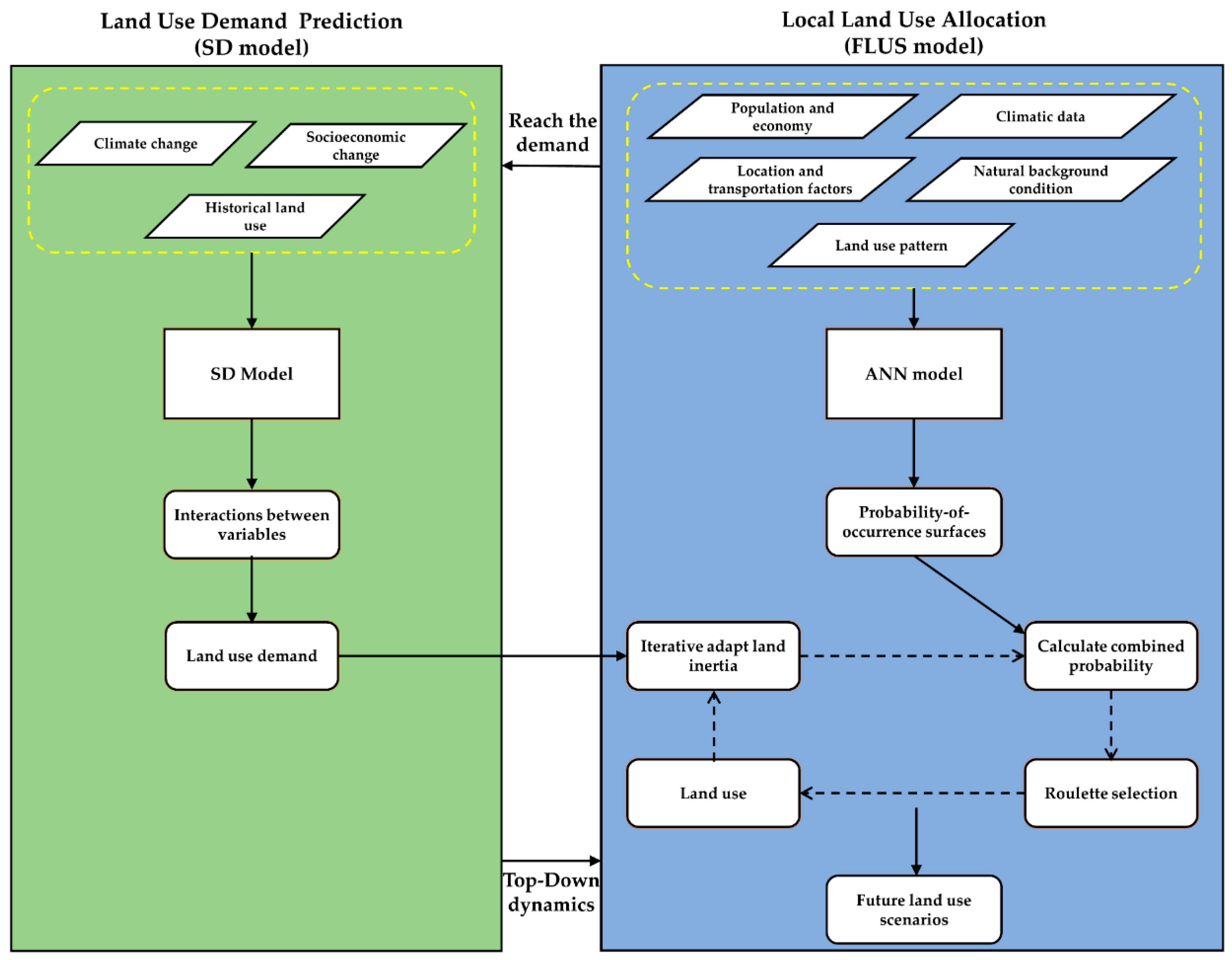
In this study, we established a coupling model for land use simulation. The realization of the coupling model consists of three steps: (1) the SD model is used to predict land use demand; (2) the FLUS model is used to simulate the spatial pattern of land use; (3) an “interactive coupling” mechanism is used to connect the SD model and the FLUS model. The general structure of the coupling model is illustrated in Figure 2.

2.2.1. Land Use Demand Prediction Using the System Dynamics (SD) Model

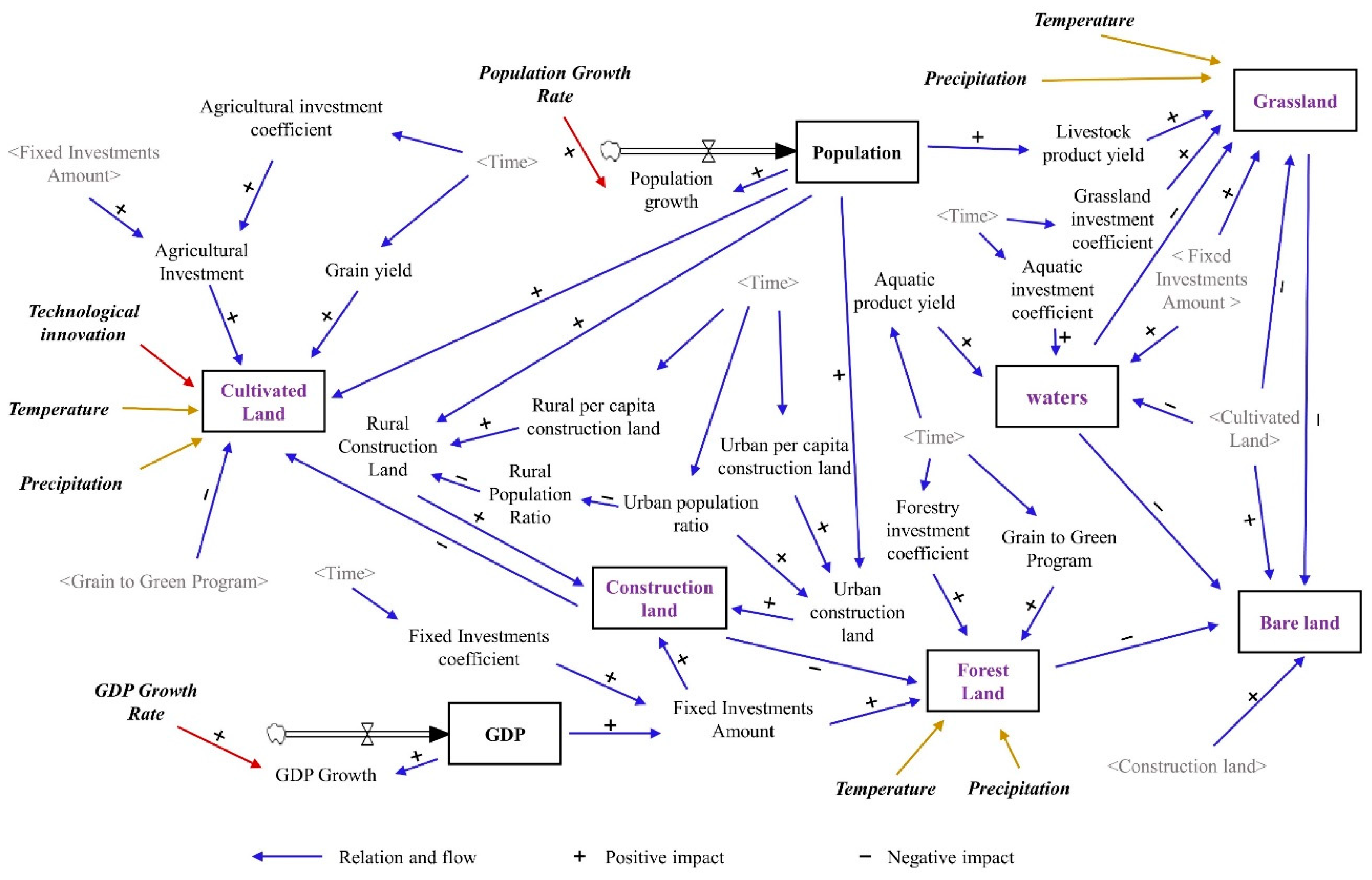
The SD model is an effective way to model complex systems’ nonlinear behavior over time through feedback loops between different modules and variables [43]. Thus, SD models can be established to understand the interaction between climate and socioeconomic changes and future land use changes. In this study, we established an SD model that considers the impact of human activities and the natural environment to predict future land use demand (Figure 3). The established SD model consists of four sectors: economy, population, climate, and land use. In the economic sector, GDP affects fixed-asset investment changes, thereby affecting the economic investment in various land use types. The population sector is very important, since population changes will directly affect the demand for agricultural and animal husbandry products, urbanization rates, and social productivity, leading to corresponding changes in other sectors. The climate sector (temperature and precipitation) is also an essential part of the model. As mentioned in the introduction, climate change has long-term effects on natural landscape dynamics. A moderate increase in precipitation and temperature can meet the water consumption and growth needs of various natural vegetation and crops, leading to changes in woodland, grassland, and cultivated land. The land use sector includes six land use types: cultivated land, forest land, grassland, construction land, waters, and bare land. The changes in each land use type are restricted by the comprehensive influence of socioeconomic and climatic conditions as well as by the interaction between various land use types. For example, the area of construction land is mainly increased by occupying cultivated land and grassland, and it will also affect the area of bare land and forest land.
The simulation time of the SD model is 2000 to 2035, and the time step is one year. The period from 2000 to 2015 is the model simulation stage, in which the collected data are used to evaluate and check the simulation results. The period from 2016 to 2035 is the simulation stage of land use scale. The 2015 data are selected as the initial simulation value, and 2016 is the starting year of the scenario simulation. The data used to build the SD model in this study include the social and economic data, such as population and GDP from 2000 to 2015, as well as the climate data, such as precipitation and temperature. Socioeconomic data were collected from China Statistical Yearbook, Shanxi Province Statistical Yearbook and Hebei Province Statistical Yearbook; climate data were provided by China Meteorological Data Network. The land use data for 2000, 2005, 2010, and 2015 were provided by the Resource and Environmental Science Data Center of the Chinese Academy of Sciences with a spatial resolution of 100 × 100 m. This model was built in Vensim PLE for windows version x64.

2.2.2. Land Use Change Spatial Pattern Simulation using the FLUS Model

The FLUS model used in this study was proposed by Sun Yat-Sen University [32]. The principle of the FLUS model is to estimate the occurrence probability of each land use type in the region based on the calculation of the land use data and the driving influence factor data in the base period by using the artificial neural network (ANN) model algorithm [44]. In this study, the ANN model will be trained with the 15 spatial driving factors in natural, social, and economic aspects that are listed in Table 1. All of the spatial datasets were resampled to the same resolution of 100 × 100 m.
In the second step, the mechanism of self-adaptive inertia and competition is adopted in the FLUS modeling process. The self-adaptive inertia coefficient is set by automatically adjusting the inheritance of the current land type for each cell based on the difference between the expected land demand and the actual land type allocated. If the development trend of a particular land type is inconsistent with the expected demand, the self-adaptive inertia coefficient will dynamically adjust the land type’s inheritance to correct the problem in the next iteration and achieve the expected goal [32]. The inertia coefficient is defined as follows:
I k t = { I k t 1 i f    | D k t 1 |      | D k t 2 | I k t 1 × D k t 2 D k t 1 i f    D k t 1 <   D k t 2 < 0 I k t 1 × D k t 1 D k t 2 i f    0 <   D k t 2 < D k t 1
where I k t denotes the inertia coefficient for land use type k at iteration time t, and D k t 1 denotes the difference between the macro demand and the allocated amount of land use type k until iteration time t − 1. The conversion cost, which indicates the conversion difficulty from the current land use type to the demand type, is obtained by analyzing historical land use change data, and it reflects the inherent attributes of land use changes [45]. The value of the conversion cost varies within the range of [0,1]. The larger the value, the more difficult the conversion.
Finally, the following formula is used to estimate the overall conversion probability of units occupied by a specific land type [46]:
T P i , k t = P i , k × Ω i , k t × I k t × Z c k
where T P i , k t denotes the overall conversion probability of grid cell i to covert from the original land use type to the demand type k at iteration time t; P i , k denotes the probability of occurrence of land use type k on grid cell i ;   Ω i , k t denotes the neighborhood influence factor of land use type k on grid cell i at iteration time t; I k t denotes the inertia coefficient of land use type k at iteration time t; and Z c k denotes the conversion cost from the original land use type c to the demand type k.
The roulette selection mechanism is used in the FLUS model to determine which land type the grid unit is converted to. In order to better simulate the dynamics and uncertainties of land use, a higher total probability has a greater chance of being assigned to the target land type, but land types with a lower probability also have a chance to be assigned to the target land type [32].

2.2.3. Integration of the SD Model with the FLUS Model

This study uses the “interactive coupling” mechanism proposed by Liang et al. [46] to closely combine the SD model and the FLUS model in order to strengthen the mutual feedback between the two models (Figure 4). The land use demand comes from the SD model’s output, which is used to guide the simulation of the land use spatial pattern of the FLUS model until the land use growth meets the forecast demand. Then, using the land use spatial pattern simulated at the previous time node, combined with the new stage’s driving factors, the SD model is used to predict the land use demand in the next period. This interaction continues throughout the simulation period, resulting in a spatial pattern map of land use in 2035.

2.3. Scenario Description and Parameterization

2.3.1. Drive Factor Setting for SD Model

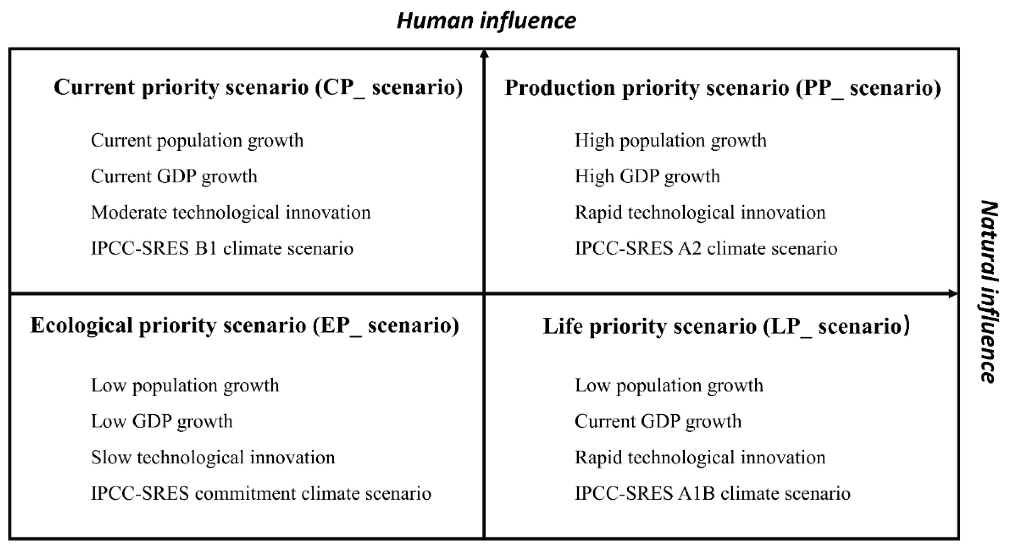
The SD model constructed in this study considers the impact of population, economy, technological innovation, and climate change on land use demand under four future scenarios from 2015 to 2035 (Figure 5). Based on the Intergovernmental Panel on Climate Change (IPCC) assessment report, four scenarios were designed, taking into account regional climate change and different socioeconomic developments in the study area [47].
We considered five parameters in different scenarios: annual economic growth, annual population growth, annual technological innovation, annual temperature growth, and annual precipitation growth. These parameters are set to be slightly different in the four scenarios to reflect the socioeconomic and natural condition differences among these scenarios (Table 2). The development trend of the economy, population, and climate change in the current priority (CP)_ scenario maintains the current growth level. This scenario’s parameters are calculated based on the statistical yearbook and meteorological data of the study area from 2000 to 2015, and they are used as reference values for other scenario parameters. In the production priority (PP)_ scenario, we assume that the establishment of Xiong’an New Area will drive its upstream area’s economic development. The population growth and economic growth are considered to experience sustained and rapid increases (1% and 20%, respectively) at the expense of many natural resources. Additionally, large-scale human activities have accelerated greenhouse gas emissions, leading to a sharp increase in temperature and precipitation. The ecological priority (EP)_ scenario focuses on protecting the ecological environment, and the population and economy in this scenario have a relatively slow growth rate (0.3% and 8%, respectively) to reduce the impact on the natural environment. The life priority (LP) scenario is a more human-oriented and sustainable development mode. In this scenario, the economy shifts to high-quality development, and the improvement of technological innovation capabilities (15%) can better meet social needs. The climate change data in the above future scenarios refer to the research of Zeng et al. because the location of the study area of Zeng et al. is adjacent to this study area, and the climate data can be used for reference [48].

2.3.2. Internal Transfer Feature Settings for FLUS Models

In this study, we designed four different conversion costs to correspond to the internal transfer characteristics of land use under different development scenarios in the future in order to meet the actual characteristics of land use conversion under different scenarios (Table 3). In the CP_ scenario, all land use types can be converted to each other. In the PP_ scenario, all land except construction land can be converted into cultivated land. In the LP_ scenario, each land is ranked according to the social development needs: construction, cultivated land, woodland, grassland, waters, and bare land. The conversion principle is implemented to prevent the conversion of high-grade land to low-grade land. In the EP_ scenario, the ecological benefits of various types of land are ranked as follows: forest land, waters, grassland, and others, and the conversion principle is the same as the LP_ scenario.

2.4. Evaluation of the Ecosystem Service Value (ESV)

In this study, we used the equivalent coefficients table of the ecosystem services proposed by Xie et al. [8] as a basis and modified the equivalent coefficients according to the actual situation of the study area. According to previous studies in the study area, we settled the correction coefficient for ESV of one standard equivalent factor as 0.70 [38]. The increase in construction land caused by rapid urbanization will cause air and water pollution, which will destroy the natural ecological environment [49,50]. Therefore, we set the service value coefficient of construction land as 0. The final value tables of the ecosystem services per unit area of different land use types were obtained (Table 4) [38]. This work was guided on “Observation Methodology for Longterm Forest Ecosystem Research” of the National Standards of the People’s Republic of China (GB/T 33027-2016).
The ESV was calculated using the following equations [51]:
E S V k = f A k × V C k f
E S V f = k A k × V C k f
E S V = k f A k × V C k f = k A k × V C k
where E S V k , E S V f and E S V refer to the ESVs of land use type k, ecosystem service function f and the entire ecosystem, respectively; A k is the area of land use type k; V C k f is the value coefficient for land use type k with the ecosystem service function f; and V C k represents the value coefficient of land use type k.

2.5. Ecological Contribution Rate of Land Use Change

The contribution rate of land use changes for ESV referring to the change rate of ESV caused by the conversion of class i land use type to class e land use type [38]. Its expression is as follows:
E L k e = ( V C e V C k ) × A k e k = 1 n e = 1 n [ ( V C e V C k ) × A k e ] × 100 %
where E L k e represents the contribution of land use change to the ecosystem service value; V C k and V C e represent the value coefficients of land use types k and e, respectively; and A k e is the area from land use type k to land use type e during the study period.

3. Results

3.1. Land Use Change in 2035

Under the different scenarios, the spatial pattern of land use in the study area is basically consistent, but changes in local areas were obvious (Figure 6). Compared with 2015, the area of each land use type was considerably different in 2035, and the degree of overall land use fragmentation was more prominent (Table 5).
Under the CP_ scenario, the areas of cultivated land, forest land, waters, construction land and bare land increased by 53.37, 353.5, 20.08, 143.64 and 0.06 km2, respectively. However, the areas of grassland decreased by 570.65 km2. It can be seen that the increase in the area of forest land and construction land mostly came from the occupation of grassland (Figure 6 and Table 6). Under the PP_ scenario, the construction land showed a dramatic growth to 330.94 km2 by 2035, almost twice that in 2015. Construction land growth was characterized by extension; that is, most of the growth was located in the periphery of the original countryside and towns, occupying a considerable amount of the cultivated land. Forest land sharply declined, with a total reduction of 353.48 km2 that mainly converted into cultivated land (Table 5 and Table 6). Under the EP_ scenario, the area of construction land increased the least among all scenarios, with an increase of only 20.62 km2. Forest land increased significantly, with a value of 565.56 km2 that mainly resulted from the transfer of grassland. Under the LP_ scenario, the area of cultivated land and construction land increased the most prominently, increasing by 53.38 and 56.18 km2, respectively, mainly due to the transfer of grassland. The areas of other land use types changed only slightly.

3.2. Changes in Ecosystem Service Values in 2035

The changes in ESV in the upstream of Xiong’an New Area under the different scenarios in 2035 are shown in Table 7. The ESV of the PP_ scenario and LP_ scenario showed a downward trend, while they increased under the EP_ scenario. The ESV of the CP_ scenario changed only slightly.
According to the type of ecosystem service, compared with 2015, the value of provisioning services increased the most in the EP_ scenario, reaching CNY 133.42 million, while the value of provisioning services in the PP_ scenario and LP_ scenario declined significantly by CNY 62.3 million and 25.21 million, respectively. The values of regulating services under the PP_ scenario and LP_ scenario decreased significantly, with decreases of CNY 1263.53 million and 438.36 million, respectively. In contrast, the value of regulating services increased significantly in the CP_ scenario and EP_ scenario, with an increase of CNY 170.59 million and 2274.14 million, respectively. The value of supporting services decreased under the CP_ scenario, PP_ scenario, and LP_ scenario, while it increased slightly under the EP_ scenario. In addition, the value of cultural services declined under both the PP_ scenario and LP_ scenario, with decreases of CNY 1635.39 million and 561.95 million, respectively. The value of cultural services increased the most in the EP_ scenario, reaching CNY 2550.59 million.
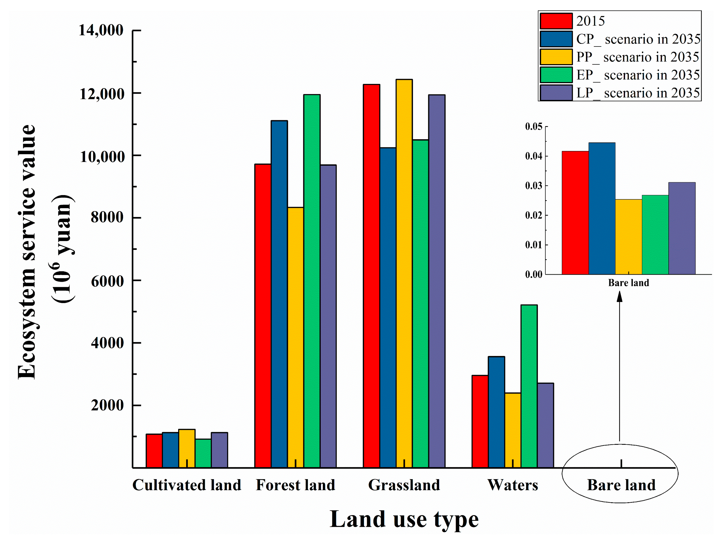
According to the land use types, compared with 2015, the ESV of cultivated land increased under the CP_ scenario, PP_ scenario, and LP_ scenario, with increases of CNY 51.24 million, 153.72 million, and 51.25 million, respectively, while it decreased under the EP_ scenario, with decreases of CNY 153.78 million (Figure 7). The ESV of forest land increased the most in the EP_ scenario, reaching CNY 2222.14 million, while the value of provisioning services in the PP_ scenario declined significantly by CNY 1388.86 million. The ESV of grassland under the PP_ scenario increased significantly, with increases of CNY 160.66 million. In contrast, the ESV of grassland decreased significantly in the CP_ scenario, EP_ scenario, and LP_ scenario with a decrease of CNY 2023.53 million, 1775.81 million, and 331.2 million, respectively. The ESV of waters increased under both the CP_ scenario and EP_ scenario, with increases of CNY 603.91 million and 2258.04 million, respectively. The value of waters services decreased the most in the PP_ scenario, reaching CNY 560.90 million. Moreover, the ESV of bare land did not significantly change.

3.3. Influence of Future Land Use Changes on Ecosystem Services Value (ESV)

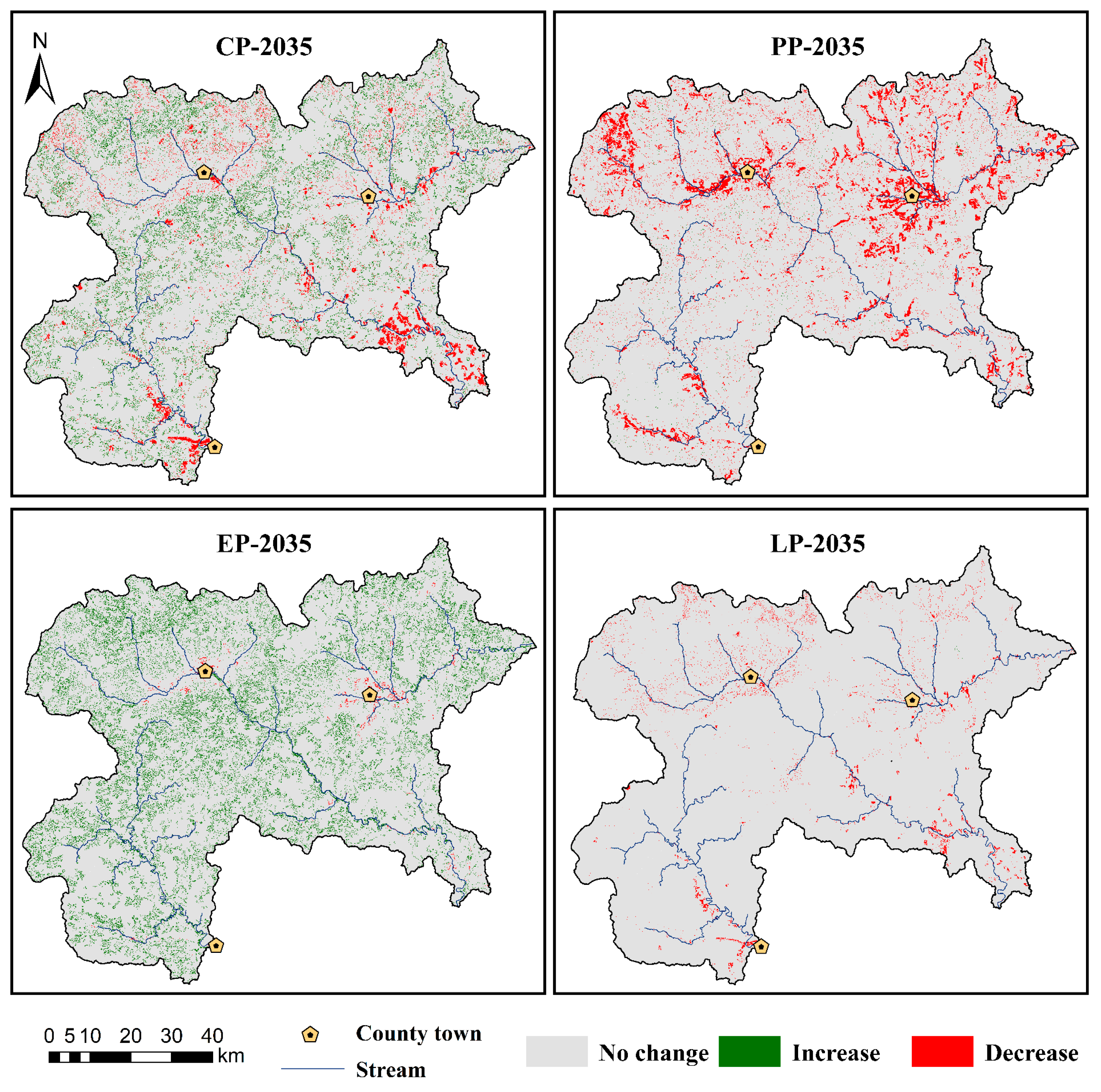
From 2015 to 2035, the area of ESV changes in the CP_ scenario, PP_ scenario, EP_ scenario and LP_ scenario was 753.83, 596.47, 781.92, and 113.66 km2, respectively (Figure 8). The area that ESV increased in the CP_ scenario and EP_ scenario was 475.19 and 761.30 km2, respectively, which mainly occurred in the region where grassland converted into forest land. The area that ESV decreased in the CP_ scenario, PP_ scenario, and LP_ scenario was 278.64, 578.14, and 113.44 km2, respectively, which mainly occurred on river banks and the surrounding areas of towns.
Quantitative calculation of the influence of land use change on ESV showed that land use change has both positive and negative effects on ESV in the study period (2015 to 2035) (Table 8). The conversion of grassland to waters was the main reason for the increase in ESV in the CP_ scenario, with a contribution rate of 74.18%. The conversion of grassland to construction land was the main reason for the decrease in ESV in the CP_ scenario, with a contribution rate of 55.70%. The conversion of forest land to cultivated land contributed the most to the total decreasing ESV in the PP_ scenario, followed by the waters converted to cultivated land. In the LP_ scenario, the conversion of grassland to construction land and the conversion of waters to cultivated land contributed 33.02% and 30.89% to the reduction of ESV, respectively. The conversion of grassland to waters played an important role in the increase in ESV in the EP_ scenario, with a contribution rate of 73.89%.

4. Discussion

4.1. Review and Synthesis Analyses of Simulation Results

This paper focuses on the impacts of land use change on ecosystem services in the upstream of Xiong’an New Area. Our results show that in the CP_ scenario, the grassland on the river bank is occupied by construction land, resulting in a decrease in ESV in the occupied area. On the contrary, the conversion of grassland to waters increases ESV in the area. Since the two trends of ESV increase and decrease occur at the same time, they offset each other within a certain range, which makes the overall change of ESV in the CP_ scenario insignificant. In the PP_ scenario and the LP_ scenario, the urbanization process and technological innovation capabilities rapidly improve, which requires an increase in construction land and cultivated land to adapt to population and economic growth [52]. Through the occupation of forest land, grassland, and waters, the area of construction land and cultivated land increases significantly, but this significantly reduces the ESV in the region. This is similar to the results of the study conducted on the Guizhou mountainous area [53] and Tianshan Mountain area [54]. Forest land and grassland can regulate regional temperature and humidity through vegetation transpiration and soil evaporation, thereby regulating the climate [55,56]. Moreover, carbon fixation and oxygen release also are among the most important services provided by the forest and grassland ecosystem [57,58]. Waters have outstanding water resource supply and hydrological regulation capabilities [59]. Therefore, when forest land, grassland, and waters are occupied by cultivated land and construction land, the ecosystem service functions in the region will decrease significantly. In the EP_ scenario, the slowdown of social and economic activities will reduce the impact of humans on the natural environment, which will make the terrestrial ecosystem and climate system form a virtuous circle, thereby accelerating the succession of vegetation. Therefore, a large amount of grassland in the EP_ scenario is converted into forest land, and the area of waters also increases significantly, which enhances the stability of the ecosystem and significantly increases ESV.
Spatially, ESV changes in most parts of the study area in the CP_ scenario. This shows that if the trends of population growth and climate change continue, the stability of the region’s ecosystem will be destroyed, which is in line with other studies carried out in other China mountains, such as the Qinling Mountains [60] and Qilian Mountains [61]. In the EP scenario, land use change positively impacts ecosystem services in most of the regions, which indicates that the “Grain-for-Green”, “ecological red line”, and other political strategies can protect ecological land and gradually improve ecosystem quality [62]. In the LP scenario, the ESV of most areas remains unchanged and only decreases in towns and river banks. In the LP_ scenario, the ESV increases significantly in the area where it decreases in the PP_ scenario. In the LP_ scenario, as the population size is controlled and technological innovation increases, resources are used efficiently. In this way, humans can meet their own needs by consuming the least natural resources, thereby reducing the scope of disturbance to the natural ecosystem [63,64]. In contrast, the population size in the PP_ scenario is not controlled, leading to increasing demand for natural resources by humans coupled with the continuous improvement in technological innovation capabilities, which ultimately leads to a sharp increase in human disturbance to the natural ecosystem area [65]. In many developing countries, economic benefits are the primary consideration in land resources management, while the ecological benefits are often ignored, which continues to increase the pressure on natural resources and ecosystems and threatens regional ecological security [66,67]. Therefore, the land transfer restriction measures and socioeconomic management policies in the LP_ scenario can provide a reference for policy makers to make sound decisions that balance the socioeconomic and ecological benefits.

4.2. Advice for Future Strategies and Policies

The water supply safety and flood controlling ability of Xiong’an New Area largely depend on the upstream ecosystem [38]. Land use changes directly affect the structure and function of the ecosystem. Therefore, it is necessary for decision makers to formulate reasonable land use strategies and policies to ensure the ecological security of the region. In order to enhance the ecological stability of the region and ensure the ecological safety of the downstream Xiong’an New Area, combined with the above research results, we suggest that focus be placed on the following aspects in future work: (1) Strict laws and regulations should be formulated in the study area to prohibit grazing, felling of trees, and occupation of waters in order to ensure that the existing ecological environment does not deteriorate. (2) Under the condition of not affecting the normal food supply, large-scale afforestation should be implemented to convert arable land and grassland into forest land. (3) The scale of construction land should be controlled, population density should be reasonably controlled, the ecological structure should be stabilized, the burden on ecosystems should be eased, and ecosystem service capability should be improved. (4) The ability to respond to climate change should be strengthened, especially in the context of rising extreme weather events, to reduce the risk of drought and flood disasters. (5) It is necessary to consider balancing the relationship between natural resources, economy, and society; strengthening cooperation between the upstream and downstream to achieve integrated river basin management; and revising the ecological environment protection strategy for a more sustainable future.

4.3. Strengths and Limitations

This study has its strengths and weakness, which we summarize here. In this study, we constructed an SD-FLUS coupling model that takes into account human activities and climate change to predict land use change, which helps to improve the accuracy of future land use change simulations. We also set different land use demands and internal transfer characteristics for different development scenarios to adapt to the various possibilities of regional land use changes. The coupling model is especially suitable for the areas which are greatly affected by human activities and climate change, such as agropastoral interlaced regions, coastal areas, and hilly regions. When applying this model to other regions, we should fully consider the characteristics the region in question and understand the interaction between climate and socioeconomic changes and future land use changes so as to establish a suitable coupling model. The equivalent coefficients table proposed by Xie et al. is suitable for ESV estimation at the national scale in China [38]. Therefore, we used the grain yield correction coefficient to make regional corrections to the equivalent coefficients table, which improved the accuracy of ESV assessment. We quantified and mapped the response of ecosystem service value to multi-scenario land use changes. The advantages of this method are its quick assessment and the low cost associated with collecting the primary data needed to achieve our objectives, which can be used for the scientific evaluation and rapid accounting of ecological assets in specific regions. This method also has strong generalizability. It can be used to comprehensively and objectively evaluate the development status of the ecological environment and future sustainable development potential of other similar regions, and it can provide theoretical support and a scientific basis for formulating relevant ecological asset compensation policies and measures.
Despite these strengths, this study also has some limitations. The limitations and accuracy of the results in this paper are mainly related to the accuracy of land use data. The land use data were provided by the Resource and Environmental Science Data Center of the Chinese Academy of Sciences with a spatial resolution of 100 × 100 m. The land use datasets do not have detailed classification [68]. For example, the grasslands of different coverage are not further differentiated, which may have an impact on the research results. Thus, to overcome these limitations, a land use dataset with high resolution is needed [69].

5. Conclusions

We predicted and evaluated ESV in the upstream of Xiong’an New Area in 2035 using the SD-FLUS coupling model and the equivalent coefficient table method. We also quantitatively calculated the impact of future land use changes on ESV under different scenarios. Based on the results, we can draw the following conclusions:
  • From 2015 to 2035, the area of construction land in the four scenarios increased. Among them, the area of construction land in the CP_ scenario and PP_ scenario is almost twice that in 2015. In the PP_ scenario, the area of forest land decreased the most, from 2474.36 km2 in 2015 to 2120.88 km2 in 2035. In the ecological scenario, the forest area increased significantly, accounting for 41.51% of the total area, and the waters had a dramatic growth to 2.37 km2 by 2035, almost twice that in 2015. In the LP_ scenario, the land use structure of the study area is relatively stable.
  • From 2015 to 2035, the ESV of the PP_ scenario and LP_ scenario showed a downward trend, while they increased under the EP_ scenario. The ESV of the CP_ scenario changed only slightly. Among the different scenarios, the value of each ecosystem service function is the smallest in the PP_ scenario, and the value of each ecosystem service function is the largest in the EP_ scenario. The ESV of cultivated land and grassland is the largest in the PP scenario, and the ESV of forest land and waters is the largest in the EP scenario.
  • From 2015 to 2035, the areas where ESV decreased mainly appeared in river banks and surrounding areas of towns. In the CP_ scenario and LP_ scenario, the conversion of grassland to construction land is the main reason for the decline in ESV, and the contribution rates are 55.70% and 33.02%, respectively. In the PP_ scenario, the conversion of forest land to cultivated land is the main reason for the decline in ESV. In the CP_ scenario and EP_ scenario, the conversion of grassland to waters is the main reason for the increase in ESV, and the contribution rates are 74.18% and 73.89%, respectively.
This study quantified the effects of land use change on ESV by evaluating the land use changes and ESVs under future scenarios in the upstream of Xiong’an New Area. The results of this study can help decision makers to optimize land use structure and promote sustainable development of the ecological environment.

Author Contributions

Conceptualization, Z.W.; methodology, Z.W.; software, Z.W.; validation, J.C.; formal analysis, Z.W.; writing—original draft preparation, Z.W.; writing—review and editing, Z.W. and J.C; visualization, Z.W.; supervision, J.C.; project administration, J.C.; funding acquisition, J.C. All authors have read and agreed to the published version of the manuscript

Funding

This research was funded by the National Natural Science Foundation of China (No. 41877170), National Key Research and Development Program of China (No. 2018YFC0406501-02) and Hebei Province Key Research and Development Program of China (No. 20324203D and No. 20536001D).

Institutional Review Board Statement

Not applicable.

Informed Consent Statement

Not applicable.

Data Availability Statement

Not applicable.

Acknowledgments

This work is supported by CFERN & BEIJING TECHNO SOLUTIONS Award Funds on excellent academic achievements.

Conflicts of Interest

The authors declare no conflict of interest.

References

  1. La Notte, A.; D’Amato, D.; Makinen, H.; Paracchini, M.L.; Liquete, C.; Egoh, B.; Geneletti, D.; Crossman, N.D. Ecosystem services classification: A systems ecology perspective of the cascade framework. Ecol. Indic. 2017, 74, 392–402. [Google Scholar] [CrossRef]
  2. Kindu, M.; Schneider, T.; Teketay, D.; Knoke, T. Changes of ecosystem service values in response to land use/land cover dynamics in Munessa-Shashemene landscape of the Ethiopian highlands. Sci. Total Environ. 2016, 547, 137–147. [Google Scholar] [CrossRef]
  3. Qian, X.; Wei, S.; Yili, Z.; Fengyun, M. Research progress in ecological carrying capacity: Implications, assessment methods and current focus. J. Resour. Ecol. 2017, 8, 514–525. [Google Scholar] [CrossRef]
  4. Song, W.; Liu, M. Farmland conversion decreases regional and national land quality in China. Land Degrad. Dev. 2016, 28, 459–471. [Google Scholar] [CrossRef]
  5. Olander, L.P.; Johnston, R.J.; Tallis, H.; Kagan, J.; Maguire, L.A.; Polasky, S.; Urban, D.; Boyd, J.; Wainger, L.; Palmer, M. Benefit relevant indicators: Ecosystem services measures that link ecological and social outcomes. Ecol. Indic. 2018, 85, 1262–1272. [Google Scholar] [CrossRef]
  6. Bateman, I.J.; Harwood, A.R.; Mace, G.M.; Watson, R.T.; Abson, D.J.; Andrews, B.; Binner, A.; Crowe, A.; Day, B.H.; Dugdale, S.; et al. Bringing ecosystem services into economic decision-making: Land use in the United Kingdom. Science 2013, 341, 45–50. [Google Scholar] [CrossRef] [PubMed]
  7. Costanza, R.; d’Arge, R.; de Groot, R.; Farber, S.; Grasso, M.; Hannon, B.; Limburg, K.; Naeem, S.; O’Neill, R.V.; Paruelo, J.; et al. The value of the world’s ecosystem services and natural capital. Ecol. Econ. 1998, 25, 3–15. [Google Scholar] [CrossRef]
  8. Xie, G.D.; Zhen, L.; Lu, C.X.; Xiao, Y.; Chen, C. Expert knowledge based valuation method of ecosystem services in China. J. Nat. Resour. 2008, 5, 911–919. [Google Scholar]
  9. Song, W.; Deng, X. Land-use/land-cover change and ecosystem service provision in China. Sci. Total Environ. 2017, 576, 705–719. [Google Scholar] [CrossRef]
  10. Liu, Y.; Hou, X.; Li, X.; Song, B.; Wang, C. Assessing and predicting changes in ecosystem service values based on land use/cover change in the Bohai Rim coastal zone. Ecol. Indic. 2020, 111, 106004. [Google Scholar] [CrossRef]
  11. Li, Y.; Zhan, J.; Liu, Y.; Zhang, F.; Zhang, M. Response of ecosystem services to land use and cover change: A case study in Chengdu City. Resour. Conserv. Recycl. 2018, 132, 291–300. [Google Scholar] [CrossRef]
  12. Koo, H.; Kleemann, J.; Fürst, C. Integrating ecosystem services into land-use modeling to assess the effects of future land-use strategies in northern Ghana. Land 2020, 9, 379. [Google Scholar] [CrossRef]
  13. Hasan, S.S.; Zhen, L.; Miah, M.G.; Ahamed, T.; Samie, A. Impact of land use change on ecosystem services: A review. Environ. Dev. 2020, 34, 100527. [Google Scholar] [CrossRef]
  14. Roces-Díaz, J.V.; Vayreda, J.; De Cáceres, M.; García-Valdés, R.; Banqué-Casanovas, M.; Morán-Ordóñez, A.; Brotons, L.; de-Miguel, S.; Martínez-Vilalta, J. Temporal changes in mediterranean forest ecosystem services are driven by stand development, rather than by climate-related disturbances. For. Ecol. Manag. 2021, 480, 118623. [Google Scholar] [CrossRef]
  15. Solé-Senan, X.O.; Juárez-Escario, A.; Robleño, I.; Conesa, J.A.; Recasens, J. Using the response-effect trait framework to disentangle the effects of agricultural intensification on the provision of ecosystem services by Mediterranean arable plants. Agric. Ecosyst. Environ. 2017, 247, 255–264. [Google Scholar] [CrossRef]
  16. Deng, C.; Liu, J.; Nie, X.; Li, Z.; Liu, Y.; Xiao, H.; Hu, X.; Wang, L.; Zhang, Y.; Zhang, G.; et al. How trade-offs between ecological construction and urbanization expansion affect ecosystem services. Ecol. Indic. 2021, 122, 107253. [Google Scholar] [CrossRef]
  17. DÍAz, S.; Lavorel, S.; McIntyre, S.U.E.; Falczuk, V.; Casanoves, F.; Milchunas, D.G.; Skarpe, C.; Rusch, G.; Sternberg, M.; Noy-Meir, I.; et al. Plant trait responses to grazing? a global synthesis. Glob. Chang. Biol. 2007, 13, 313–341. [Google Scholar] [CrossRef]
  18. Deng, X.; Shi, Q.; Zhang, Q.; Shi, C.; Yin, F. Impacts of land use and land cover changes on surface energy and water balance in the Heihe River Basin of China, 2000–2010. Phys. Chem. Earth Parts A/B/C 2015, 79–82, 2–10. [Google Scholar] [CrossRef]
  19. Zhong, L.; Wang, J.; Zhang, X.; Ying, L. Effects of agricultural land consolidation on ecosystem services: Trade-offs and synergies. J. Clean. Prod. 2020, 264, 121412. [Google Scholar] [CrossRef]
  20. Hou, X.; Liu, J.; Zhang, D.; Zhao, M.; Xia, C. Impact of urbanization on the eco-efficiency of cultivated land utilization: A case study on the Yangtze River Economic Belt, China. J. Clean. Prod. 2019, 238, 117916. [Google Scholar] [CrossRef]
  21. Song, W.; Deng, X.; Yuan, Y.; Wang, Z.; Li, Z. Impacts of land-use change on valued ecosystem service in rapidly urbanized North China Plain. Ecol. Model. 2015, 318, 245–253. [Google Scholar] [CrossRef]
  22. Aguirre-Gutierrez, J.; Malhi, Y.; Lewis, S.L.; Fauset, S.; Adu-Bredu, S.; Affum-Baffoe, K.; Baker, T.R.; Gvozdevaite, A.; Hubau, W.; Moore, S.; et al. Long-term droughts may drive drier tropical forests towards increased functional, taxonomic and phylogenetic homogeneity. Nat. Commun. 2020, 11, 3346. [Google Scholar] [CrossRef] [PubMed]
  23. Runting, R.K.; Bryan, B.A.; Dee, L.E.; Maseyk, F.J.; Mandle, L.; Hamel, P.; Wilson, K.A.; Yetka, K.; Possingham, H.P.; Rhodes, J.R. Incorporating climate change into ecosystem service assessments and decisions: A review. Glob. Chang. Biol. 2017, 23, 28–41. [Google Scholar] [CrossRef] [Green Version]
  24. Jiao, S.; Li, J.; Li, Y.; Xu, Z.; Kong, B.; Li, Y.; Shen, Y. Variation of soil organic carbon and physical properties in relation to land uses in the Yellow River Delta, China. Sci. Rep. 2020, 10, 20317. [Google Scholar] [CrossRef] [PubMed]
  25. Gao, J.; O’Neill, B.C. Mapping global urban land for the 21st century with data-driven simulations and Shared Socioeconomic Pathways. Nat. Commun. 2020, 11, 2302. [Google Scholar] [CrossRef] [PubMed]
  26. Gao, Y.; Tian, L.; Cao, Y.; Zhou, L.; Li, Z.; Hou, D. Supplying social infrastructure land for satisfying public needs or leasing residential land? A study of local government choices in China. Land Use Policy 2019, 87, 104088. [Google Scholar] [CrossRef]
  27. Dietrich, J.P.; Schmitz, C.; Lotze-Campen, H.; Popp, A.; Müller, C. Forecasting technological change in agriculture—An endogenous implementation in a global land use model. Technol. Forecast. Soc. Chang. 2014, 81, 236–249. [Google Scholar] [CrossRef]
  28. Xu, X.; Du, Z.; Zhang, H. Integrating the system dynamic and cellular automata models to predict land use and land cover change. Int. J. Appl. Earth Obs. Geoinf. 2016, 52, 568–579. [Google Scholar] [CrossRef]
  29. Geng, B.; Zheng, X.; Fu, M. Scenario analysis of sustainable intensive land use based on SD model. Sustain. Cities Soc. 2017, 29, 193–202. [Google Scholar] [CrossRef]
  30. Shen, Q.; Chen, Q.; Tang, B.-S.; Yeung, S.; Hu, Y.; Cheung, G. A system dynamics model for the sustainable land use planning and development. Habitat Int. 2009, 33, 15–25. [Google Scholar] [CrossRef]
  31. Wang, Y.; Li, S. Simulating multiple class urban land-use/cover changes by RBFN-based CA model. Comput. Geosci. 2011, 37, 111–121. [Google Scholar] [CrossRef]
  32. Liu, X.; Liang, X.; Li, X.; Xu, X.; Ou, J.; Chen, Y.; Li, S.; Wang, S.; Pei, F. A future land use simulation model (FLUS) for simulating multiple land use scenarios by coupling human and natural effects. Landsc. Urban. Plan. 2017, 168, 94–116. [Google Scholar] [CrossRef]
  33. Halmy, M.W.A.; Gessler, P.E.; Hicke, J.A.; Salem, B.B. Land use/land cover change detection and prediction in the north-western coastal desert of Egypt using Markov-CA. Appl. Geogr. 2015, 63, 101–112. [Google Scholar] [CrossRef]
  34. Kamusoko, C.; Aniya, M.; Adi, B.; Manjoro, M. Rural sustainability under threat in Zimbabwe—Simulation of future land use/cover changes in the Bindura district based on the Markov-cellular automata model. Appl. Geogr. 2009, 29, 435–447. [Google Scholar] [CrossRef]
  35. Ma, S.; Li, X.; Cai, Y. Delimiting the urban growth boundaries with a modified ant colony optimization model. Comput. Environ. Urban. Syst. 2017, 62, 146–155. [Google Scholar] [CrossRef]
  36. Li, X.; Chen, G.; Liu, X.; Liang, X.; Wang, S.; Chen, Y.; Pei, F.; Xu, X. A new global land-use and land-cover change product at a 1-km resolution for 2010 to 2100 based on human–environment interactions. Ann. Am. Assoc. Geogr. 2017, 107, 1040–1059. [Google Scholar] [CrossRef]
  37. Samat, N.; Mahamud, M.A.; Tan, M.L.; Maghsoodi Tilaki, M.J.; Tew, Y.L. Modelling land cover changes in peri-urban areas: A case study of george town conurbation, Malaysia. Land 2020, 9, 373. [Google Scholar] [CrossRef]
  38. Wang, Z.; Cao, J.; Zhu, C.; Yang, H. The impact of land use change on ecosystem service value in the upstream of Xiong’an new area. Sustainability 2020, 12, 5707. [Google Scholar] [CrossRef]
  39. Yang, D.; Liu, W.; Tang, L.; Chen, L.; Li, X.; Xu, X. Estimation of water provision service for monsoon catchments of South China: Applicability of the InVEST model. Landsc. Urban. Plan. 2019, 182, 133–143. [Google Scholar] [CrossRef]
  40. Zhao, G.; Zhou, H.; Liu, X.; Li, K.; Zhang, P.; Wen, W.; Yu, Y. PHAHs in 14 principal river sediments from Hai River basin, China. Sci. Total Environ. 2012, 427–428, 139–145. [Google Scholar] [CrossRef]
  41. Yang, T.; Liu, J.; Chen, Q.; Zhang, J.; Yang, Y. Estimation of environmental flow requirements for the river ecosystem in the Haihe River Basin, China. Water Sci. Technol. 2013, 67, 699–707. [Google Scholar] [CrossRef] [PubMed]
  42. Song, C.; Ke, L.; Pan, H.; Zhan, S.; Liu, K.; Ma, R. Long-term surface water changes and driving cause in Xiong’an, China: From dense Landsat time series images and synthetic analysis. Sci. Bull. 2018, 63, 708–716. [Google Scholar] [CrossRef] [Green Version]
  43. Coyle, R.G. System dynamics modelling: A practical approach. J. Oper. Res. Soc. 1997, 48, 544. [Google Scholar] [CrossRef]
  44. Li, X.; Yeh, A.G.-O. Neural-network-based cellular automata for simulating multiple land use changes using GIS. Int. J. Geogr. Inf. Sci. 2002, 16, 323–343. [Google Scholar] [CrossRef]
  45. Huang, K.; Liu, X.; Li, X.; Liang, J.; He, S. An improved artificial immune system for seeking the Pareto front of land-use allocation problem in large areas. Int. J. Geogr. Inf. Sci. 2013, 27, 922–946. [Google Scholar] [CrossRef]
  46. Liang, X.; Liu, X.; Li, X.; Chen, Y.; Tian, H.; Yao, Y. Delineating multi-scenario urban growth boundaries with a CA-based FLUS model and morphological method. Landsc. Urban. Plan. 2018, 177, 47–63. [Google Scholar] [CrossRef]
  47. Sohl, T.L.; Sleeter, B.M.; Sayler, K.L.; Bouchard, M.A.; Reker, R.R.; Bennett, S.L.; Sleeter, R.R.; Kanengieter, R.L.; Zhu, Z. Spatially explicit land-use and land-cover scenarios for the Great Plains of the United States. Agric. Ecosyst. Environ. 2012, 153, 1–15. [Google Scholar] [CrossRef] [Green Version]
  48. Zeng, S.; Zhang, L.; Xia, J.; Yang, Z. Water cycle characteristic and its responses to climate change of the yongding River Basin. J. Basic Sci. Eng. 2013, 21, 501–511. [Google Scholar]
  49. Lin, X.; Lu, C.; Song, K.; Su, Y.; Lei, Y.; Zhong, L.; Gao, Y. Analysis of coupling coordination variance between urbanization quality and eco-environment pressure: A case study of the west taiwan strait urban agglomeration, China. Sustainability 2020, 12, 2643. [Google Scholar] [CrossRef] [Green Version]
  50. Kuai, P.; Li, W.; Liu, N. Evaluating the effects of land use planning for non-point source pollution based on a system dynamics approach in China. PLoS ONE 2015, 10, e0135572. [Google Scholar] [CrossRef]
  51. Xie, G.; Zhang, C.; Zhen, L.; Zhang, L. Dynamic changes in the value of China’s ecosystem services. Ecosyst. Serv. 2017, 26, 146–154. [Google Scholar] [CrossRef]
  52. Cao, M.; Zhu, Y.; Lü, G.; Chen, M.; Qiao, W. Spatial distribution of global cultivated land and its variation between 2000 and 2010, from both agro-ecological and geopolitical perspectives. Sustainability 2019, 11, 1242. [Google Scholar] [CrossRef] [Green Version]
  53. Zhao, Y.; Li, X. Spatial Correlation between type of mountain area and land use degree in Guizhou province, China. Sustainability 2016, 8, 849. [Google Scholar] [CrossRef] [Green Version]
  54. Fang, C.; Gao, Q.; Zhang, X.; Cheng, W. Spatiotemporal characteristics of the expansion of an urban agglomeration and its effect on the eco-environment: Case study on the northern slope of the Tianshan Mountains. Sci. China Earth Sci. 2019, 62, 1461–1472. [Google Scholar] [CrossRef]
  55. Vieira, J.; Matos, P.; Mexia, T.; Silva, P.; Lopes, N.; Freitas, C.; Correia, O.; Santos-Reis, M.; Branquinho, C.; Pinho, P. Green spaces are not all the same for the provision of air purification and climate regulation services: The case of urban parks. Environ. Res. 2018, 160, 306–313. [Google Scholar] [CrossRef]
  56. Scheller, R.; Parajuli, R. Forest management for climate change in New England and the Klamath ecoregions: Motivations, practices, and barriers. Forests 2018, 9, 626. [Google Scholar] [CrossRef] [Green Version]
  57. Chu, X.; Zhan, J.; Li, Z.; Zhang, F.; Qi, W. Assessment on forest carbon sequestration in the Three-North Shelterbelt Program region, China. J. Clean. Prod. 2019, 215, 382–389. [Google Scholar] [CrossRef]
  58. Vass, M.M.; Elofsson, K. Is forest carbon sequestration at the expense of bioenergy and forest products cost-efficient in EU climate policy to 2050? J. For. Econ. 2016, 24, 82–105. [Google Scholar] [CrossRef] [Green Version]
  59. Sun, Z.; Lotz, T.; Chang, N.B. Assessing the long-term effects of land use changes on runoff patterns and food production in a large lake watershed with policy implications. J. Environ. Manag. 2017, 204, 92–101. [Google Scholar] [CrossRef]
  60. Zhang, H.; Gao, Y.; Hua, Y.; Zhang, Y.; Liu, K. Assessing and mapping recreationists’ perceived social values for ecosystem services in the Qinling Mountains, China. Ecosyst. Serv. 2019, 39, 101006. [Google Scholar] [CrossRef]
  61. Qian, D.; Yan, C.; Xiu, L.; Feng, K. The impact of mining changes on surrounding lands and ecosystem service value in the Southern Slope of Qilian Mountains. Ecol. Complex. 2018, 36, 138–148. [Google Scholar] [CrossRef]
  62. Verburg, R.; Selnes, T.; Verweij, P. Governing ecosystem services: National and local lessons from policy appraisal and implementation. Ecosyst. Serv. 2016, 18, 186–197. [Google Scholar] [CrossRef] [Green Version]
  63. Mao, D.; He, X.; Wang, Z.; Tian, Y.; Xiang, H.; Yu, H.; Man, W.; Jia, M.; Ren, C.; Zheng, H. Diverse policies leading to contrasting impacts on land cover and ecosystem services in Northeast China. J. Clean. Prod. 2019, 240, 117961. [Google Scholar] [CrossRef]
  64. Zhang, J.; Yin, N.; Wang, S.; Yu, J.; Zhao, W.; Fu, B. A multiple importance–satisfaction analysis framework for the sustainable management of protected areas: Integrating ecosystem services and basic needs. Ecosyst. Serv. 2020, 46, 101219. [Google Scholar] [CrossRef]
  65. Ye, Y.; Bryan, B.A.; Zhang, J.; Connor, J.D.; Chen, L.; Qin, Z.; He, M. Changes in land-use and ecosystem services in the Guangzhou-Foshan Metropolitan Area, China from 1990 to 2010: Implications for sustainability under rapid urbanization. Ecol. Indic. 2018, 93, 930–941. [Google Scholar] [CrossRef]
  66. Clements, H.S.; De Vos, A.; Bezerra, J.C.; Coetzer, K.; Maciejewski, K.; Mograbi, P.J.; Shackleton, C. The relevance of ecosystem services to land reform policies: Insights from South Africa. Land Use Policy 2021, 100, 104939. [Google Scholar] [CrossRef]
  67. Rosa, I.M.D.; Purvis, A.; Alkemade, R.; Chaplin-Kramer, R.; Ferrier, S.; Guerra, C.A.; Hurtt, G.; Kim, H.; Leadley, P.; Martins, I.S.; et al. Challenges in producing policy-relevant global scenarios of biodiversity and ecosystem services. Glob. Ecol. Conserv. 2020, 22, e00886. [Google Scholar] [CrossRef]
  68. Wang, Y.; Dai, E.; Yin, L.; Ma, L. Land use/land cover change and the effects on ecosystem services in the Hengduan Mountain region, China. Ecosyst. Serv. 2018, 34, 55–67. [Google Scholar] [CrossRef]
  69. Arowolo, A.O.; Deng, X.; Olatunji, O.A.; Obayelu, A.E. Assessing changes in the value of ecosystem services in response to land-use/land-cover dynamics in Nigeria. Sci. Total Environ. 2018, 636, 597–609. [Google Scholar] [CrossRef]
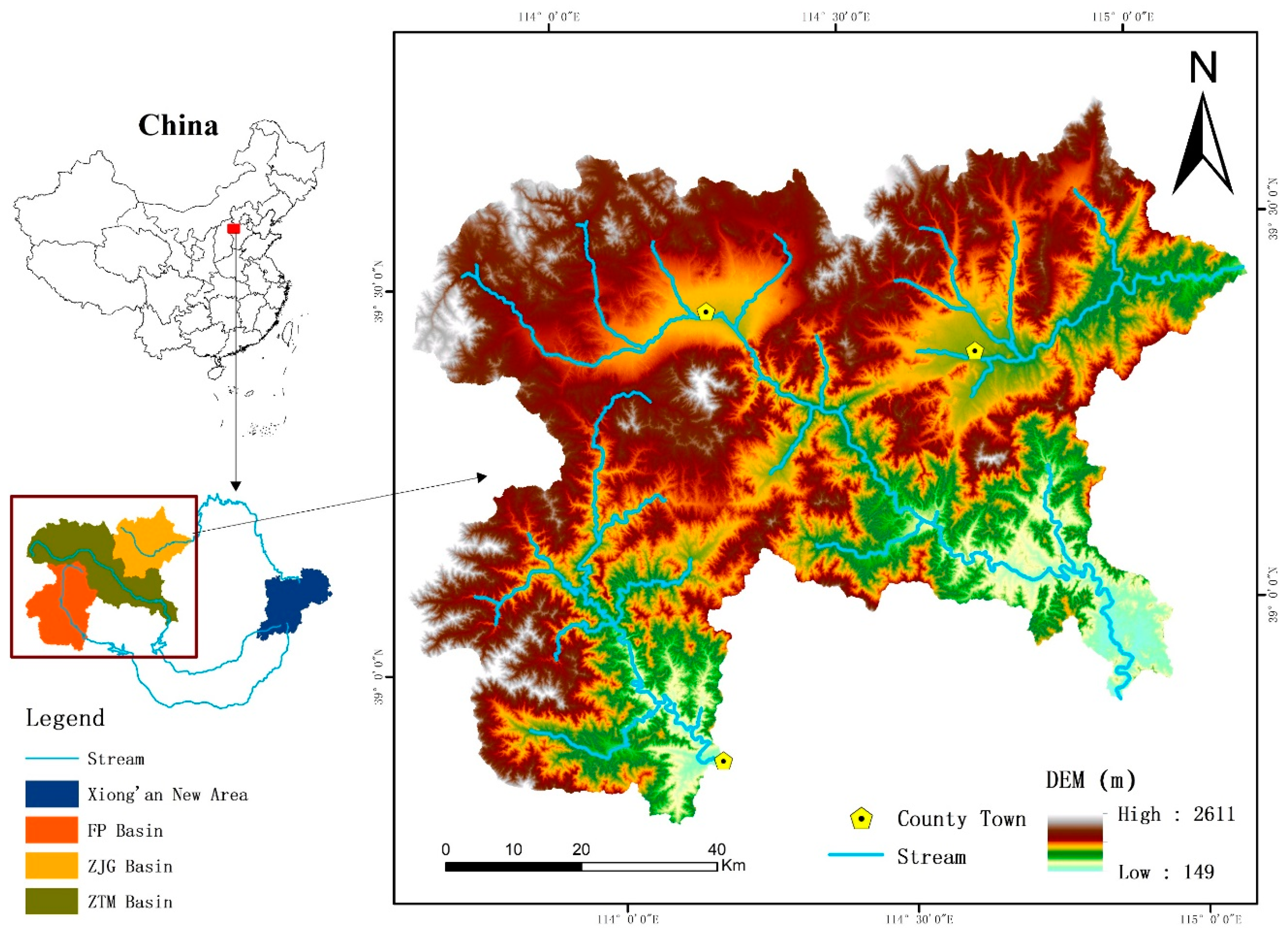
Figure 1. Geographical location of the study area.
Sustainability 13 00704 g001
Figure 2. The flowchart of the integrated system dynamics (SD) and future land use simulation (FLUS) model.
Sustainability 13 00704 g002
Figure 3. The structure of the SD model.
Sustainability 13 00704 g003
Figure 4. Interactive coupling mechanism of the SD and FLUS models.
Sustainability 13 00704 g004
Figure 5. Configurations of four development scenarios with regard to human and natural effects.
Sustainability 13 00704 g005
Figure 6. Simulated spatial pattern of land use in the four designed scenarios in 2035.
Sustainability 13 00704 g006
Figure 7. Ecosystem service value of different land use types under the four future scenarios.
Sustainability 13 00704 g007
Figure 8. Spatial distribution map of ecosystem service value changes under the four future scenarios.
Sustainability 13 00704 g008
Table 1. Data on driving forces of land use change.
CategoryDataYearResolutionData Resource
Social economyPopulation20101 kmGlobal Change Research Data Publishing & Repository
Gross Domestic Product (GDP)20101 kmGlobal Change Research Data Publishing & Repository
TerrainDigital Elevation Model (DEM)201030 mGeospatial Data Cloud
Aspect201030 mCalculated from DEM
Slope201030 mCalculated from DEM
Traffic and streamNational road2010VectorNational catalogue service for geographic information
Provincial road
Highway
Railway
River net
ClimateAnnual mean temperature2000–2010100 mChina Meteorological Data Network (Spatial interpolation)
Annual mean precipitation
Table 2. Parameterization of the socioeconomic and natural factors in the four designed scenarios.
ParametersCP_ ScenarioPP_ ScenarioEP_ ScenarioLP_ Scenario
Annual economic growth (%/a)13.882088
Annual population growth (%/a)0.5310.30.53
Annual technological innovation (%/a)1015515
Annual precipitation growth (%/a)0.040.170.030.20
Annual temperature growth (%/a)0.020.030.020.04
Table 3. Conversion cost matrix under the four future scenarios.
CP_ ScenarioPP_ ScenarioEP_ ScenarioLP_ Scenario
abcdefabcdefabcdefabcdef
a111111100010111111100010
b111111111001010000110010
c111111111111011100101010
d111111101101000100111110
e111111000010000010000010
f111111111111111111111111
Note: a, b, c, d, e, and f represent cultivated land, forest land, grassland, waters, construction land, and bare land, respectively; 0 means conversion is not possible, and 1 means conversion is allowed.
Table 4. Ecosystem service value per unit area for different land use types in the upstream of Xiong’an New Area.
Ecosystem Service FunctionsCultivated LandForest LandGrasslandWatersBare Land
Provisioning servicesFood production2035.18502.81694.361915.460.00
Raw material production957.731149.281005.62550.700.00
Water supply47.89598.58550.7019,849.000.00
Regulating servicesGas regulation1604.203735.153543.611843.6347.89
Climate regulation861.9611,133.639385.775483.020.00
Environment purification 239.433328.123088.6913,288.53239.43
Hydrological regulation646.477997.066871.7324,4796.3071.83
Supporting servicesSoil conservation2466.164525.284333.742226.7347.89
Nutrient cycle maintenance287.32359.15335.21167.600.00
Biodiversity311.264142.193926.706105.5447.89
Cultural servicesAesthetic landscape143.661819.691723.924525.2823.94
Total9601.2639,290.9635,460.0330,0751.79478.87
Table 5. Areas of six land use types in 2015 and under the four future scenarios in 2035 (km2).
20152035
CP_ ScenarioPP_ ScenarioEP_ ScenarioLP_ Scenario
Cultivated land1120.821174.191280.92960.661174.2
Forest land2474.362827.862120.883039.922466.81
Grassland3460.342889.693505.652959.553366.94
Waters98.28118.3679.63173.3689.89
Construction land163.88307.52330.94184.5220.06
Bare land0.870.930.530.560.65
Table 6. Land use transition matrix under the four future scenarios from 2015 to 2035 (km2).
Land Use in 2035.Land Use in 2015
123456Transfer in
CP_ scenario11092.499.2557.026.199.24081.7
22.932414.13409.680.280.840413.73
322.8449.252814.751.091.740.0274.94
40.20.1727.5190.460.02027.9
52.361.56151.30.26152.040155.48
6000.08000.850.08
Transfer out28.3360.23645.597.8211.840.02
PP_ scenario1964.31275.3329.2711.900.11316.61
202102.7217.98000.1818.16
3091.123411.013.4700.0594.64
400079.63000
5156.515.192.083.28163.880167.06
6000000.530
Transfer out156.51371.6449.3318.6500.34
EP_ scenario1960.66000000
215.552474.36549.86000.15565.56
3120.502838.89000.16120.66
43.49071.5998.280075.08
520.62000163.88020.62
6000000.560
Transfer out160.160621.45000.31
LP_ scenario11119.216.0842.945.970054.99
202466.2600.4400.110.55
30033651.8300.111.94
400089.89000
51.612.0252.40.15163.88056.18
6000000.650
Transfer out1.618.195.348.3900.22
Note: 1, 2, 3, 4, 5, and 6 represent cultivated land, forest land, grassland, waters, construction land, and bare land, respectively.
Table 7. Ecosystem service values of the upstream of Xiong’an New Area under the four future scenarios (CNY 106).
Ecosystem Service Functions20152035
CP_ ScenarioPP_ ScenarioEP_ ScenarioLP_ Scenario
Provisioning servicesFood production611.62604.47626.00587.07614.01
Raw material production745.11734.57723.35748.54739.50
Water supply539.11568.96484.20693.65517.12
Total1895.841908.001833.542029.261870.63
Regulating servicesGas regulation2348.352290.432254.622370.282319.44
Climate regulation6153.166026.745805.716340.166057.09
Environment purification2049.742019.101925.142179.222008.51
Hydrological regulation6834.937220.506137.198770.666562.78
Total17,386.1817,556.7716,122.6519,660.3216,947.82
Supporting servicesSoil conservation2917.642847.942812.642933.762885.04
Nutrient cycle Maintenance238.71234.15231.82238.89236.70
Biodiversity2478.602414.872343.562557.072435.33
Total5634.945496.955388.035729.725557.07
Cultural servicesAesthetic landscape1107.371083.171044.721155.631086.86
Total1107.371083.171044.721155.631086.86
Total26,024.3326,044.8924,388.9428,574.9225,462.38
Table 8. The contribution rate of land use change to ecosystem service value (ESV) under the four future scenarios from 2015 to 2035.
Change PatternTypes of Land Use ChangeContribution Rate/%
CP_ ScenarioPP_ ScenarioEP_ ScenarioLP_ Scenario
Improvement of ecosystem function1→20.88 1.80
1→36.00 12.12
1→40.59 3.95
2→40.45
3→215.9587.618.20
3→474.18 73.89
5→10.90
5→20.34
5→30.63
5→40.06
6→1 1.28
6→2 8.890.0252.60
6→30.012.220.0247.40
Total100.00100.00100.00100.00
Deterioration of ecosystem function1→50.249.14100.000.27
2→12.8549.75 3.21
2→31.962.12
2→50.641.24 1.41
3→115.314.61 19.73
3→555.700.45 33.02
3→60.03
4→118.7121.08 30.89
4→20.76 2.04
4→33.005.60 8.63
4→50.816.00 0.80
Total100.00100.00100.00100.00
Note: 1, 2, 3, 4, 5, and 6 represent cultivated land, forest land, grassland, waters, construction land, and bare land, respectively; 1→2 represents the conversion of cultivated land to forest land, and so on for other codes.
Publisher’s Note: MDPI stays neutral with regard to jurisdictional claims in published maps and institutional affiliations.