The Impact of Land Use Change on Water-Related Ecosystem Services in the Bashang Area of Hebei Province, China

Abstract

Land use change is an important scientific issue recognized for its potential to alter ecosystem services (ESs), especially water-related ecosystem services (WRESs). Using the integrated valuation of ecosystem services and trade-offs (InVEST) model, this study quantified and mapped spatiotemporal variations in land use and corresponding WRESs in the Bashang area of Hebei Province, China (BAHP) to investigate how land use change impacted WRESs by means of scenario analysis, especially, in which a new evaluation indicator, average ecology effect (AEE) was proposed and well applied. The results indicated that woodland expansion (+602.61 km²) and grassland shrinkage (−500.57 km²) dominated the land use change in the BAHP in 2000–2018, which altered local WRESs, including the moderate declines in water purification and water yield, as well as a significant enhancement in soil conservation. In scenario analysis, compared to baseline levels, riparian woodland buffer and planting trees scenarios slightly decreased water yield but strengthened water purification and soil conservation; reclaiming wasteland and integrated development scenarios significantly enhanced soil conservation but lowered water yield and water purification; fertilizer reduction scenario effectively mitigated water deterioration. According to AEE, the riparian woodland buffer (RWB) scenario performed greater than the planting trees (PT) scenario on variations of WRESs per unit area, which differed completely from the results based on total variations. Overall, a multiple-scale indicator for a comprehensive evaluation of ESs should receive more attention.

1. Introduction

Ecosystem services (ESs) represent the varieties of benefits that ecosystem offered to humanity directly or indirectly to maintain living and welfare, in the form of culture, provisioning, regulating, and supporting services [1,2]. As the Intergovernmental Science–Policy Platform on Biodiversity and Ecosystem Services (IPBES) reported, under the influence of human activities, global ecosystems are suffering from ESs losses at an unprecedented speed [3], thus arousing growing attention in ESs worldwide [4,5]. The reduction of ESs, especially the water-related ecosystem services (WRESs), e.g., water yield [6], soil conservation [7], and water purification [8], would severely threaten human health and welfare. Hence, utilizing and maintaining ESs sustainably is a hot but challenging issue [9,10]. Land use change was an essential factor to recognize its potential impacts on ESs through altering land use type, pattern, and intensity [11,12]. For instance, the conversions of land use types could affect ESs provision by disturbing ecological processes, including hydrological cycle, soil deposition, and material exchange [2]. Regarding land use patterns, higher landscape fragmentation was proven to have a negative impact on ESs [13]. Besides, high-level land use intensity (e.g., high-level urbanization and agricultural expansion) generally had a negative impact on most ESs [2]. The existing studies have demonstrated that land use change resulted in a series of ecological problems, such as water quality degradation, soil erosion, and water supply reduction [2,14].

Despite the increasing interest in ESs, there is no standardized framework to illustrate the mechanism of how land use change impacts ESs [15]. Most studies tried to value ESs and then to explain the relationship between ecosystem service value and land use change [16,17], which was essentially similar to the weighted summation of corresponding parameters based on each land use type. Besides, scenario analyses were commonly used to investigate the impact of land use change on ESs [18], of which the key step was scenario setting. Some studies selected the past land use landscapes as alternative scenarios and then evaluated the relative impacts of land use and climate change on ESs by fixing climate conditions [19,20]. Such a method only explained the past dynamics of ESs and provided limited information to serve future decision-making. Based on this, considerable studies tended to utilize the projection models (e.g., CA-Markov model, CLUE-S model [21], and econometric model [11]) to simulate future scenarios associated with local ecological policies and plans. However, it still remained defective to use projection models when the systematic errors of these models far exceed realistic land use change, especially for a relatively small spatial scale. In fact, these approaches to create scenarios exposed a common shortcoming—the created scenarios included multiple land use conversions while using the above-mentioned methods, thus leading to the uncertainty of which kind of land use conversion could be responsible for changes in ESs. Accordingly, a few scholars began designing the future scenarios based on the current land use landscape [22,23] (e.g., returning degraded cropland land to woodland or grassland, developing cropland on areas with lower slope). The approach to design scenarios could effectively quantify the impacts of one or more specific land use conversions on future ESs, and helped enhance ESs provision [24].

Indeed, the selection of ecological models was critical in the process of investigating related issues. The widely used models mainly included Artificial Intelligence for Ecosystem Services (ARIES) model, Soil and Water Assessment Tool (SWAT) model, the Integrated Valuation of Ecosystem Services and Trade-offs (InVEST) model, and so on. The ARIES model featured discerning the key elements in ecosystem service flow and capable of mapping spatial locations and quantities of these elements [25], but only to cater for the explanation of biophysical relationships [26]. The SWAT model, based on detailed hydrological processes and expert knowledge, could stimulate high-scale results while requiring a heavy workload [27]. In contrast, the InVEST model neither required many model parameters nor involved complicated calculation steps, thereby quite appropriate for multiple-scale assessments of ESs due to its operability and practicalness. Such studies were conducted in regional [21,28] and national scales [29].

Hence, this study utilized the InVEST model as the main tool to reveal how land use change drove WRESs in the Bashang area of Hebei Province (BAHP), a typical arid and semi-arid area in northern China. Water resources for the whole world were commonly recognized as the most important limiting factor for economic development and ecological security in arid or semi-arid areas. Here, the BAHP as a water-deficient area, as well as an ecologically vulnerable area, has developed long-term vegetable planting and consumed substantial water resources since the implementation of the Grain for Green Program in 2000 [30]. Moreover, under the interference of human activities (e.g., excessive groundwater exploitation, agricultural irrigation, and so on), most open waters shrunk or even dried up, and groundwater levels also showed a significant decline locally [31]. Under the current situation, the limited water resources could hardly continue to provide enough WRESs to meet local residents‘ demands. In order to cope with this water crisis, the Government of Hebei Province launched a new plan for land use in 2019 [32], aiming to facilitate the construction of water conservation areas and ecological environment support areas and ensure the local ecological security, as well as sustainable water resources. Therefore, studies on better understanding the impact of land use change on local WRESs is necessary to help policymakers formulate optimal schemes in advance and bridge the knowledge gap between WRESs and land use change.

In this study, three WRESs, including water purification, water yield, and soil conservation in the BAHP from 2000 to 2018, were quantified and mapped by the InVEST model. Besides, five alternative scenarios and a base landscape (baseline) based on land use in 2018 were developed into scenario analyses. The objectives of this study were (1) to assess the spatiotemporal dynamics of land use and WRESs; (2) to analyze the impacts of future scenarios on WRESs; and (3) to reveal the potential mechanism of how land use change impacted WRESs in arid and semi-arid area and provided a reference for related studies in other similar areas.

2. Materials and Methods

2.1. Study Area

The BAHP (40°70′–42°60′ N, 113°70′–117°90′ E) is located in the northwestern part of Hebei Province, China and across six counties (e.g., Guyuan, Zhangbei, Kangbao, Shangyi, Weichang, and Fengning), with a total area of 1.9 × 10⁴ km² and an elevation range of 831–2215 m (Figure 1). The BAHP is featured by numerous seasonal rivers and more lakes. Nowadays, most lakes and rivers are in danger of drying up because of a fast decline in groundwater levels led by human activities [31]. The ever largest plateau inland lake in northern China—the Anguli Lake, had totally degenerated into saline-alkali land in 2004. The BAHP belongs to continental monsoon plateau climate; the annual average temperature is 1–2 °C, and the annual average precipitation is approximately 400 mm, with nearly 70% of the rainfall appearing from June to September [30]. In the past several decades, the BAHP has experienced a long-term and high-intensity vegetable planting owing to agricultural transformation under the stimulation of the market economy, which causes a huge consumption of local water resources and seriously threatens water ecological environment. The BAHP is confronting a series of water-related ecological problems, including soil erosion, water shortage, water quality deterioration, and so on.

2.2. Data Sources and Pre-Processing

The main data used in this study and their sources are introduced as follows: (1) 30-m resolution land use datasets in 2000 and 2018 were from the Resource and Environment Science Data Center of Chinese Academy of Sciences; They are divided into six land use types, including cropland, woodland, grassland, water, construction land and unused land; (2) A digital elevation model (DEM) data, ASTER GDEM 30M, was obtained from the Geospatial Data Cloud (http://www.gscloud.cn); (3) 1-km resolution soil data, namely, Harmonized World Soil Database (HWSD), was from the National Cryosphere Desert center (http://www.crensed.ac.cn); (4) meteorological data (e.g., daily precipitation and evaporation data) were from China Meteorological Data Service Center (http://data.cma.cn), including the data of 11 meteorological stations in and around the BAHP; raster maps of meteorological data were derived from the interpolation utilizing the Kriging tool in ArcMap10.2 software; (5) the vector map of sub-watershed was extracted by Hydrological Analysis tool in ArcMap10.2 software.

2.3. Analysis of Land Use Changes and Scenario Settings

2.3.1. Water Yield

Water yield is based on water balance principles, obtained by subtracting the actual annual evapotranspiration from the annual precipitation in each grid [33]. The calculation was based on the Budyko curve [34], and the water yield module algorithm in the InVEST model is as follows:

$$Y_x=\left(1-\frac{AE{T}_x}{P_x}\right)\times P_x$$

(1)

where Y_x is the water yield of grid x, AET_x is the annual actual evapotranspiration on grid x, and P_x is the annual precipitation in grid x.

2.3.2. Soil Conservation

Soil export, an opposite representation to soil conservation, is calculated based on the Universal Soil Loss Equation (USLE) [35]. In terms of sediment retention, the InVEST model takes the important hydrological process into account, in which sediment in the upper slope can be intercepted, making the final results more scientific and reasonable [33]. The average soil export rate on pixel x is quantified by the following:

$$USL{E}_x=R_x\times K_x\times L{S}_x\times C_x\times P_x$$

(2)

where, USLE_x is the annual soil loss of grid x; R_x is the rainfall-runoff erosivity of grid x, K_x is the soil erodibility factor of grid x, LS_x is the slope-length factor of grid x, C_x is the crop management factor of grid x, and P_x is the support practice factor of grid x.

2.3.3. Water Purification

Water purification, a critical regulating service, measured by the annual nitrogen or phosphorus exports based on the corresponding export coefficient of each land use type; it represents the capacity of the ecosystem in purifying water quality by retaining non-point source pollutants through the effect of soil and vegetation [33]. The average nitrogen export at grid-scale was calculated in the InVEST model by the following equations:

$$AL{V}_x=HS{S}_x\times po{l}_x$$

(3)

$$HS{S}_x=\frac{{\lambda }_x}{\overline{{\lambda }_x}}$$

(4)

$${\lambda }_x=\log \left({\displaystyle {\sum }_U{Y}_U}\right)$$

(5)

where ALV_x is the adjusted loading value of grid x; HSS_x is the hydrologic sensitivity score of grid x, and pol_x is the output coefficient of grid x; λ_x is runoff index of grid x; $\overline{{\lambda }_x}$ is mean runoff index in the study area; Σ_UY_U is the sum of the water yield of the grid along the flow path above grid x.

2.4. New Indicator—Average Ecology Effect

In scenario analyses, a common indicator—total value variations of ecosystem services—was often utilized to evaluate how much one scenario affects ESs. Consequently, a consensus was that the smaller the total values of ESs changed, the more slight this scenario performed. In some cases, the area of some regions where land use was altered by one scenario rule is limited, thus causing a small fluctuation in total values of ESs, but actually, these local regions generated intense impacts on ESs under this scenario. To quantify this part of impacts, we proposed a new indicator, Average Ecology Effect (AEE). AEE aimed to quantify per unit area of ESs variations only for the part of land use change and to provide a new evaluation indicator to compare different scenarios’ impacts on ESs. However, the limitation of AEE was that it was only applicable to the scenario where only one land use type came into being as a result of land use change. The formula of AEE is as follows:

$$AE{E}_i=\frac{\Delta E{S}_i}{\Delta S}$$

(6)

where AEE_i is the unit area variation of ecosystem service i under one scenario, and its unit depends on the unit of ecosystem service i; ΔES_i is the total variation of ecosystem service i under one scenario; ΔS is the area variation of desired land use type under one scenario. (unit: ha).

2.5. Scenario Setting

In order to simulate the future impacts of land use change on WRESs, this study designed five alternative scenarios relevant to local land use planning to estimate WRESs in each scenario; besides, land use in 2018 was assumed as a baseline for further comparison among different scenarios. The detailed process was displayed in

Table 1. Different scenarios setting.

Scenarios	Descriptions	Variations
Baseline (2018)	Land use in 2018 (No treatment)
Riparian woodland buffer (RWB) Scenario	100-m-wide riparian buffer is converted into woodland (excluding construction land).	(1) cropland = −0.76%; (2) woodland = +4.1%; (3) grassland = −1.01%; (4) unused land = −3.08%
Planting trees (PT) Scenario	Cropland and unused land that have a slope gradient of >15° were converted into woodland.	(1) cropland = −2.38%; (2) woodland = +7.28% (3) unused land = −0.26%
Reclaiming wasteland (RW) Scenario	Unused land that has a slope gradient of <6° were converted into cropland for agricultural development, but woodland and grassland with a slope gradient of <6° were not converted due to eco-environmental protection.	(1) cropland = +9.29%; (2) unused land = −94.47%
Integrated development (ID) Scenario	Combine RWB, PT and RW scenarios. The priorities are as follows: RWB > PT > RW	(1) cropland = +5.22%; (2) woodland = +13.44% (3) grassland = −2.04%; (4) unused land = −94.92%
Fertilizer reduction (FR) Scenario	The nutrient loading of cropland reduce by 20%	Nitrogen loading of cropland decrease from 22.02 kg/ha to 16.16 kg/ha.

.

3. Results

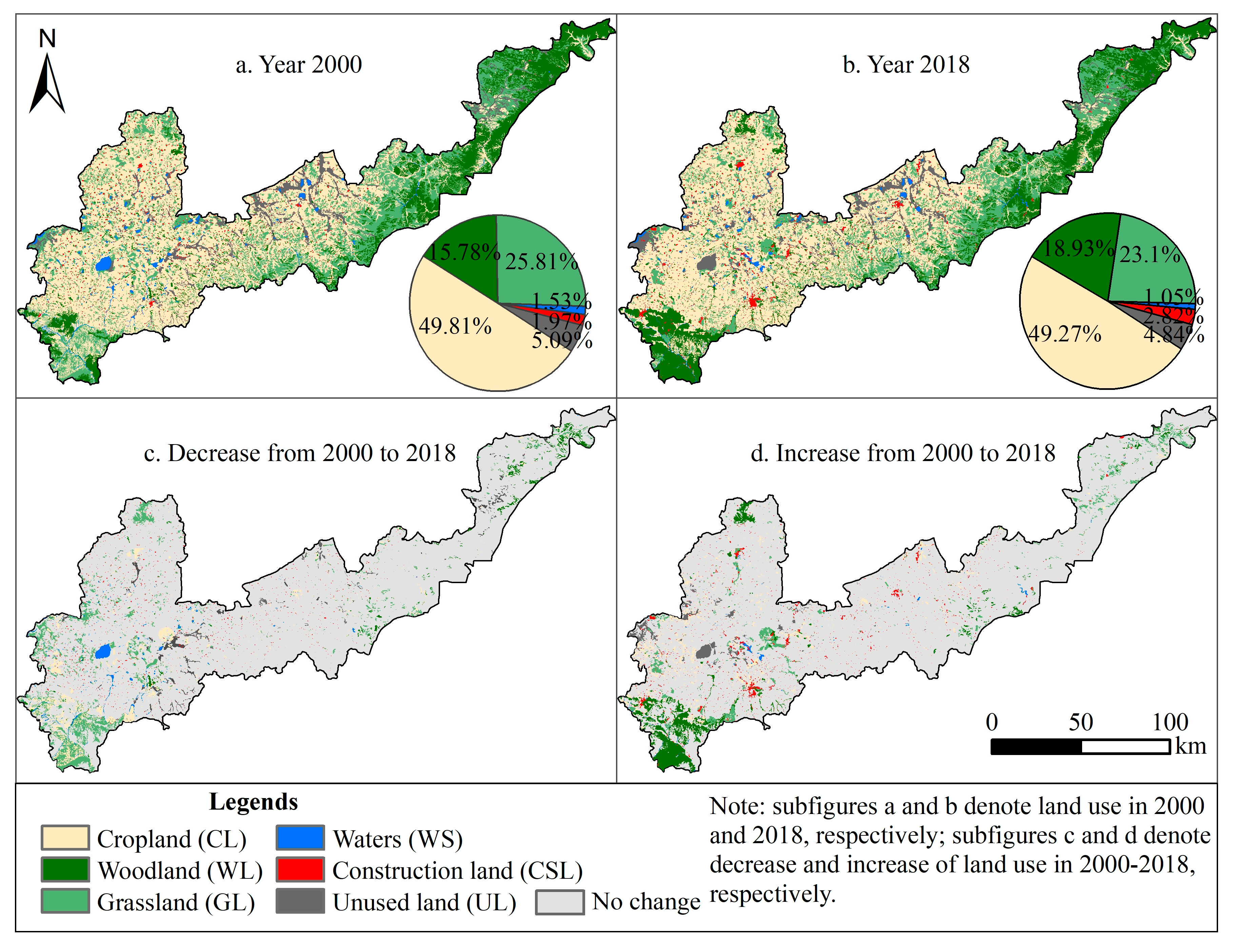
3.1. Land Use Change in the BAHP from 2000 to 2018

Maps of land use in 2000 and 2018 were displayed in Figure 2. On the whole, six land use types kept decreasing except for woodland and construction land. Among them, cropland was the primary land use type, accounting for the highest proportion (49.27%) of the entire BAHP in 2018, and showed only a 1.07% decrease from 2000. Accordingly, although waters and construction land occupied the least proportion of the total area in 2018 (1.05% and 2.82%, respectively), their change rates were the highest compared with the other four land use types, reaching −31.75% and 43.16%, respectively. Over the past 18 years, the area of woodland expansion and that of grassland shrinkage were 602.61 km² (+16.60%) and 500.57 km² (−11.30%), respectively, dominating the most main land use change for the BAHP. Regarding unused land, it covered more than 929 km² in 2018 and decreased by 5.08% compared with 2000. Generally, land use change in the BAHP from 2000 to 2018 was characterized by a high change rate in both construction land and waters, and significant area change in woodland and grassland.

From 2000 to 2018, the distribution pattern of land use and its spatial change varied among the six counties in the BAHP. In 2018, croplands were mainly distributed in Zhangbei (30.41%), Kangbao (24.86%), Guyuan (21.25%) and Shangyi (13.58%), and decreased by 31.55% and 48.26% in Shangyi and Zhangbei, with new 32.85% and 30.28% increases from 2000, respectively. Nearly 83.03% of Woodland and 53.63% of grassland were mainly observed in Fengning, Weichang, and Shangyi in 2018, respectively. Among them, grassland shrunk appeared primarily in western BAHP, and woodlands expansion was located in Shangyi (71.31%). Waters were mainly found in Guyuan (25.56%), Shangyi (24.90%), and Zhangbei (23.76%) whose most distinct change was the disappearance of Anguli Lake. Construction lands concentrated mainly in the urban core region of every county and extended outwards over the past two decades. Unused lands occurred mainly in Guyuan (40.71%) and Zhangbei (20.07%), and its spatial change in Zhangbei could be described as “a decrease in the east, but an increase in the west”.

From 2000 to 2018, the conversion from cropland to woodland and grassland reached 230.97 km² and 191.19 km², respectively (

Table 2. Land use conversion matrix from 2000 to 2018 unit: km².

2018	2000
	Cropland	Woodland	Grassland	Waters	Construction land	Unused land	Total
Cropland	8885.68	51.29	295.63	24.33	115.27	76.05	9448.25
Woodland	230.97	2802.43	534.96	29.18	2.35	29.62	3629.51
Grassland	191.19	150.49	3906.83	19.86	20.75	140.56	4429.68
Waters	18.45	2.89	15.52	148.89	1.15	13.84	200.74
Construction land	201.59	17.6	67.06	3.39	229.15	22.15	540.94
Unused land	22.36	2.20	130.25	68.48	9.18	696.53	929.00
Total	9550.24	3026.9	4950.25	294.13	377.85	978.75	19,178.12

). In addition, nearly 201.59 km² of construction land came mainly from cropland. In the same period, approximately 295.63 km², 534.96 km², and 130.25 km² of grassland were transformed to cropland, woodland, and unused land, respectively. Moreover, the area of waters degenerating into unused land was 68.48 km², which was caused primarily by the drying up of the Anguli Lake (Figure 2c). Besides, newly grown grassland (140.56 km²) and cropland (76.05 km²) were both converted from unused land. It could be concluded that the local government had made some progress in revegetation practices. However, notably, such success was at the expense of a dramatic decline in grassland.

3.2. Evaluation of WRESs Based on Past Land Use Changes

Water yield was a critical provision service for the BAHP, a semi-arid area, and its supply shortage would seriously threaten the local water resources sustainability and ecology security. Driven by land use change, the water yield increased from 29.64 × 10⁸ m³ in 2000 to 29.76 × 10⁸ m³ in 2018, an increase of only 0.40% (Figure 3). This was mainly related to precipitation and land use change. On the one hand, water yield was highly sensitive to variations in precipitation [36], whereas this study used annual average precipitation to eliminate meteorological influences on water yield. On the other hand, there was a trade-off between afforestation and urbanization for their impacts on water yield, finally causing a slight net increase.

Water purification was also modestly improved, as nitrogen export reached 6.37 × 10⁶ kg in 2018, showing a 0.93% decrease from 2000. Although ever-increasing construction land produced high nitrogen exports, newly generated woodlands in practice intercepted more nutrients, resulting in a positive influence on water quality.

Soil conservation in the BAHP was significantly strengthened due to a 14.05% decrease in soil exports during the past 18 years. By 2018, total soil export was reduced to 5.14 × 10⁶ tons. Generally, woodland possessed the strongest soil retention capacity among all land use types, however, it was the only land use type to maintain the growth trend except for construction land in BAHP during 2000–2018. Hence, woodland expansion was reasonably identified as the main factor for the enhancement of soil retention.

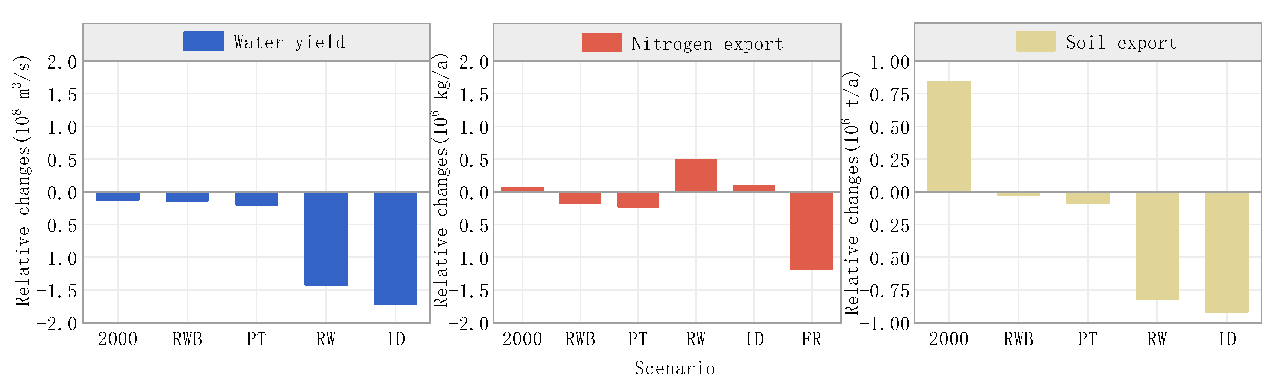
3.3. The Comparison of WRESs in Five Future Scenarios

In this study, we selected the land use in 2018 as a baseline. Figure 3 displayed the relative variations of WRESs among different alternative scenarios. The riparian woodland buffer (RWB) scenario performed well in soil conservation and water purification because of the slight declines in nitrogen export (−2.83%) and soil export (−0.58%), respectively, but it performed poorly on water yield because water supply decreased by 0.47% compared with the baseline level. The planting trees (PT) scenario generated similar effects on WRESs with the RWB scenario, and as compared with the baseline, soil export, nitrogen export, and water yield further decreased by 0.67%, 3.61%, and 1.75%, respectively. These were mainly because under the PT and RWB scenarios, the expansion of woodland led to the overall increases in evapotranspiration, nutrient interception capacity, and sediment retention capacity. Besides, for woodland, the litter layer on its soil surface also effectively slowed down the runoff accumulation and direct erosion from rainwater, thereby avoiding more sediment and nutrient losses.

As unused land with a slope below 6° was transformed to cropland, the reclaiming wasteland (RW) scenario performed worse on water yield due to a 4.81% decrease compared with the baseline, which mainly resulted from higher evapotranspiration of vegetation coverage in cropland. Similarly, the RW scenario also showed a worse performance on water purification because nitrogen export was 7.70% higher than that in the baseline, at a total value of 6.86 × 10⁶ kg/a, indicating that a high proportion of cropland generated more nitrogen sources and nutrient exports. However, different from the previous two, soil conservation in the RW scenario exhibited a significantly increasing trend by a dramatic decline of 15.95% (0.82 × 10⁶ tons) in soil loss compared with the baseline level, which was mainly due to the large gap between cropland and unused land on soil retention capacity.

Regarding the integrated development (ID) scenario, it performed best in soil conservation due to a minimum value of 4.22 × 10⁶ kg/a in sediment export but did worse in water yield, which was also because of a minimum value of 28.04 m³/a in the water supply. Compared with baseline, the ID scenario slightly degraded water purification as a result of a 1.41% increase in nitrogen export.

Finally, we added an extra fertilizer reduction (FR) scenario to investigate whether it would effectively mitigate water quality deterioration. The result was interesting because the FR scenario exhibited the largest decline in nitrogen export (−18.68%), far more than that in other scenarios. We attributed this to the high proportion of cropland in the BAHP (more than 49%) and its high nitrogen loading (20.02 kg/ha) before the implementation of fertilizer reduction. This result released a message that limiting the use of chemical fertilizers in cropland was an effective means for controlling pollutant emissions.

3.4. The Spatial Distribution Pattern of WRESs in Baseline and Five Future Alternative Scenarios

Figure 4 showed the spatial distribution of per unit area of WRESs in different scenarios based on a subwatershed scale (Figure 1). For water yield, its reductions occurred in subwatershed 5 under the RWB scenario and subwatershed 4 under the PT scenario, respectively, because high evapotranspiration of woodland resulted in reductions of the surface water in these regions. In addition, water yield in the RW scenario followed the spatial changes similar to that in the ID scenario, and under these two scenarios, subwatershed 5 and 11 jointly experienced declines in water yield, as a higher proportion of unused land was replaced by cropland and contributed to more evapotranspiration compared to other subwatersheds.

For water purification, there was no significant spatial difference observed in the distribution pattern of nitrogen export between the PT scenario and the baseline. Under the RWB scenario, the only decrease occurred in subwatershed 7, as the large area of woodland buffer was applied near waters in this region and strengthened the nutrient export control. In the RW scenario, the nitrogen exports increased mainly in subwatershed 5, 8, 9, and 11 because unused land located here was almost converted to cropland, thus contributing to a larger amount of nutrient export. The ID scenario performed similarly to the RW scenario in the spatial change of nitrogen export, except in subwatershed 8 and 11, which indicated that vegetation restoration mitigated water quality deterioration in these two regions because of the RW scenario. Finally, the FR scenario showed a declining trend in the subwatershed 4, 5, 7, 8, and 11 compared to the baseline level, as these five subwatersheds covered almost the entire cropland of the BAHP, decreasing nitrogen loading in cropland and further limited nitrogen exports from nutrient sources.

Regarding soil conservation, as compared to the baseline level, spatial differences in soil export were not obvious enough to be captured in both RWB and PT scenarios. However, in RW and ID scenarios, the reductions in soil export were observed in subwatershed 2 and 5, and this was mainly because frequent conversions of unused land to cropland took place in these regions and generated more positive effects on soil erosion control.

3.5. Comparison of AEE Among Three Scenarios

The values of AEE in RWB, PT, and RW scenarios were calculated in

Table 3. The values of average ecology effect (AEE) in three scenarios.

Scenarios	AEEWY (m3·ha−1)	AEENE (kg·ha−1)	AEESE (t·ha−1)
RWB	−931.84	−11.98	−2.00
PT	−589.73	−6.78	−2.65
RW	−1629.33	5.58	−9.34

Notes: WY = water yield; NE = nitrogen export; SE = soil export.

. ID and FR scenarios are excluded due to the limitation of AEE. The AEE_WY in RW scenario (−1629.33) was significantly lower than that in RWB (−931.84) and PT (−589.73) scenarios, which meant per unit area of the conversion from unused land to cropland in RW scenario exhibited a stronger negative effect on water yield than the corresponding conversions in both RWB and RW scenarios.

For water purification, the value of AEE_NE in the RWB scenario was −11.98 kg/ha, 76.70% lower than that in the PT scenario, indicating that the afforestation efforts in riparian buffer performed better on the removal of nutrients than that in a steep slope. The value of AEE_NE in the RW scenario reached 5.58 kg/ha, which represented that per hectare of the substitute of unused land by cropland would lead to an extra 5.58 kg nitrogen output.

Regarding soil conservation, the values of AEE_SE in RWB, PT, and RW scenarios were −2.00, −2.65, and −9.34 t/ha, respectively. The RW scenario performed best in AEE_SE compared with PT and RWB scenarios, and significantly improved soil erosion control after wasteland reclamation. The result suggested that in unit area, planting trees on steeper slopes could more effectively decrease soil loss than that in the riparian buffer.

4. Discussion

4.1. Linking Land Use Change and WRESs in the Past 18 Years

Land use change affected WRESs mainly by altering the properties, processes, and components of the ecosystem (e.g., evapotranspiration, nutrient interception, and sediment retention capacity) [37]. Indeed, the potential mechanism between land use change and WRESs was more complex and still poorly understood [38]. In this paper, annual average values (e.g., precipitation and evapotranspiration) were used to eliminate the extremes of meteorological data and ensured land use change as the only influencing factor (similar to previous studies [22,39]), because we focused more on the impact of land use change on WRESs. During the past 18 years, the BAHP experienced drastic woodland expansion (+602.61 km²) and grassland shrinkage (−520.57 km²), including highly relative urbanization growth (43.16%), which indicated that afforestation projects in the BAHP conducted by the local policy-makers had made great progress and generated positive effects on water yield (a 0.40% increase), water purification (a 0.93% decline in nitrogen export), and soil conservation (a 14.05% decline in soil export). Most notably, these positive impacts on WRESs were purely derived from land use change in the BAHP. The study [20] pointed out that compared to land use change, climate change has a stronger influence on water yield and weaker impacts on soil conversation and nitrogen export. Another study [40] also demonstrated that climate factors had a highly positive relationship with water yield. The change levels among WRESs in this study were basically consistent with the above-mentioned study results. Here, it could be acknowledged that land use change has a stronger impact on soil conservation than that on water yield and water purification in the BAHP, an arid and semi-arid area.

4.2. Implications of WRESs in the BAHP Based on Scenario Analysis and AEE

In order to understand the impacts of one or several special land use conversions on WRESs, we created one baseline and five alternative scenarios to compare the output results of these scenarios by the InVEST model. In view of the total value changes of WRESs, RWB and PT scenarios slightly enhanced water purification and soil conservation but reduced water yield because of the expansion of woodland (similar to previous studies [22,23]). In addition, we found that the RW scenario, similar to the agricultural expansion scenario proposed in previous studies [22,23,41], generated an opposite conclusion—the RW scenario significantly enhanced soil conservation due to a significant reduction (15.95%) in soil export compared with the baseline level. This was primarily because the RW scenario did not transform vegetation types (i.e., woodland and grassland) to cropland, namely, a kind of special agricultural development strategy taking ecology protection into account. Although the RW scenario greatly improved agricultural production (a 9.29% increase in cropland), as a consequence, it aggravated water quality deterioration (a 7.70% increase in nitrogen export) because of high nitrogen loading in the cropland [42]. The ID scenario resulted in the largest reductions in both water yield (−5.78%) and soil export (−17.90%), and an increase of 1.41% in nitrogen export, which was basically accepted because more foods were provided at the expense of relatively slight water quality degradation. Notably, water yield reduction did not mean the total lessening of ESs provision, because existing studies demonstrated revegetation (including afforestation) could reduce water yield [43,44] and even generate positive effects on the hydrological cycle by accelerating the exchange of water vapor [45]. Finally, the additional FR scenario showed a massive reduction (−18.68%) in nitrogen export and significantly strengthened soil conservation, which meant that the FR scenario could be applied to the ID scenario and effectively made up for the deficiency of water purification, thus deserving to be the optimal measure to enhance WRESs provision in the BAHP.

In this study, in view of total value changes of WRESs, RWB and PT scenarios, similar to scenarios used in previous studies [23,41], generated relatively small impacts on WRESs. In reality, this was mainly because there were quite limited areas suitable for the implementations of RWB and PT scenarios in the BAHP. Besides, the PT scenario performed greater on WRESs due to the higher increase of woodland in the PT scenario (+7.28%) than that in the RWB scenario (+4.10%). To make the two scenarios comparable, not just depending on the only indicator such as total value change of WRESs, AEE was proposed to provide new insights on assessing the impacts of different scenarios on WRESs. The final results showed that the RWB scenario performed better than the PT scenario in per unit area of water yield reduction and water purification totally different from the results derived from total variations of WRESs in the previous section. This finding suggested an important message that inconsistent results may be produced based on different evaluation indicators when assessing one or more kinds of ESs. Such a suggestion could be reflected in this study in which afforestation around the riparian buffer was more appropriate in views of its improvement on water purification and hydrological cycle. Accordingly, afforestation on steep slopes was more beneficial to soil erosion control than that on the riparian buffer.

This study made contributions in highlighting the importance of spatial heterogeneity on issues about geography science and ecology science, and revealing a necessity for cautious assessment on ESs. Exactly, land use structure and topography often varied in different study areas, thus determining different land uses and ESs provisions from the same scenario. For example, the study [41] showed that cropland as the main land use type made agriculture expansion scenario (similar to RW scenario in this study) perform most greatly on WRESs. Moreover, when the study area [22,46] was featured with low average slopes and cropland was not the primary land use type, the agriculture expansion scenario also exhibited a stronger impact on WRESs than other scenarios. The above-mentioned study, consistent with our results, jointly indicated spatial heterogeneity was worth considering in similar issues. Besides, multiple evaluation indicators could result in diverse conclusions because of spatial heterogeneity, for instance, there were distinct differences between AEE and total value variations in the explanations on how much various scenarios impacted WRESs. A similar result was also reasonably concluded based on another study [47], which exhibited that the PT scenario performed evidently better than the RWB scenario on soil conservation due to reductions of 50.64% and 30.05% in soil exports, respectively, but showed a narrow gap on enhancing soil conservation in views of AEE_SE in PT (0.74 t/ha) and RWB (0.80 t/ha) scenarios. As available data was quite limited in other similar studies, more verification of AEE needs to be conducted in the future.

4.3. Limitations and Prospects

The InVEST model simplified hydrological processes, therefore there were many uncertainties for realistic simulation. For instance, the water yield model did not consider the annual variation of runoff generation and concentration. However, the generation of hydropower depends on the flow regulation, the nutrient retention model did not involve any biochemical reaction, and the sediment delivery ratio model also ignored the sediment sources from landslides and river courses [33]. Despite the limitations, the InVEST model was widely identified as a suitable tool for multiple ecosystem services assessments due to less input data and relatively high accuracy [48,49]. Due to the absence of data in the BAHP, a further field study needed to be carried out to validate the results calculated by the InVEST model in the future. Even so, approaches and results in this study still supported a more comprehensive understanding of the driving mechanisms of how land use change impacted WRESs and informed decision-makers and stakeholders of alternative land use planning to serve optimal WRESs provision.

ESs assessment was the frontier and hot spot of ecology science and geography science, and it was the bridge and link between natural processes and human processes [12]. However, the challenges on ecosystem service science still exist, including that (1) formulating a scientific framework used for explaining the relationship between ecosystem processes and services under different land use change driven scenarios; (2) developing multiple indicators to comprehensively assess ESs provision, trades off and synergies, driver factor and so on; and (3) integrating ESs assessments into spatial planning to accomplish the combination of science-policy because all are difficult and require new interdisciplinary knowledge.

5. Conclusions

This study evaluated land use change and three WRESs in the BAHP from 2000 to 2018, including water yield, soil conservation, and water purification (in terms of soil export and nitrogen export). In addition to scenario analysis, a new indicator was put forward in order to further compare the impacts of different scenarios on WRESs. The results indicated that from 2000 to 2018, the BAHP mainly experienced a significant increase in woodland (602.61 km²) converted primarily from grassland (534.96 km²) and a rapid urbanization expansion (+43.16%) at the expense of cropland and grassland, ultimately leading to the corresponding alterations in WRESs. From 2000 to 2018, WRESs in the BAHP were characterized by a slight improvement in water yield (+0.40%), significant enhancement in soil conservation (a 14.04% decrease in soil export), and a moderate degeneration in water purification (a 6.69% decrease in soil export). For scenario analysis, in views of the total value variations of WRESs, as compared to the RWB scenario, the PT scenario performed better in water purification and soil conservation but had worse performance on water yield. In addition, compared with the baseline, both PT and ID scenarios performed significantly well in soil conservation because of obvious declines (more than 15.95%) in soil export but performed relatively poorly in water yield and water purification. We found that the FR scenario effectively mitigated water quality deterioration as a result of an obvious decline (−18.68%) in nitrogen export, which suggested that nutrient loading parameters in the InVEST model had strong impacts on output results of nutrient export. Notably, the new indicator, AEE, indicated the opposite results. AEE indicated that the RWB scenario actually performed greater on water yield and water purification compared with the PT scenario, as both AEE_WY (−931.84) and AEE_NE (−11.98) in the RWB scenario were smaller than AEE_WY (−589.73) and AEE_NE (−6.78) in the PT scenario, which was different from conclusions drawn by total value variations of WRESs in the previous section. Based on the above-mentioned analysis, three important points were made: (1) Afforestation in the riparian buffer could improve relatively higher ESs provision than that on steep slopes in views of the unit area; (2) Integrating the FR scenario into the ID scenario could effectively mitigate more nitrogen exports in the ID scenario; (3) Multiple-scale indicators should be developed into a comprehensive assessment on ESs, so as to avoid a one-sided conclusion.

References

1. Costanza, R.; d’Arge, R.; de Groot, R.; Farber, S.; Grasso, M.; Hannon, B.; Limburg, K.; Naeem, S.; O’Neill, R.V.; Paruelo, J.; et al. The value of the world’s ecosystem services and natural capital. Nature 1997, 387, 253–260. [Google Scholar] [CrossRef]
2. Millennium Ecosystem Assessment. Ecosystems and Human Well-Being: Synthesis; Island Press: Washington, DC, USA, 2005. [Google Scholar]
3. Intergovernmental Science-Policy Platform on Biodiversity and Ecosystem Services (IPBES). Summary for Policymakers of the Global Assessment Report on Biodiversity and Ecosystem Services of the Intergovernmental Science-Policy Platform on Biodiversity and Ecosystem Services. Bonn, Germany. 2019. Available online: https://ipbes.net/global-assessment-report-biodiversity-ecosystem-services (accessed on 8 October 2019).
4. Braat, L.C.; Groot, R.D. The ecosystem services agenda: Bridging the worlds of natural science and economics, conservation and development, and public and private policy. Ecosyst. Serv. 2012, 1, 4–15. [Google Scholar] [CrossRef] [Green Version]
5. Keesstra, S.; Nunes, J.; Novara, A.; Finger, D.; Avelar, D.; Kalantari, Z.; Cerdà, A. The superior effect of nature based solutions in land management for enhancing ecosystem services. Sci. Total Environ. 2018, 610, 997–1009. [Google Scholar] [CrossRef] [PubMed] [Green Version]
6. Zhuang, C.; Ouyang, Z.Y.; Xu, W.; Bai, Y.; Zhou, W.; Zheng, H.; Wang, X. Impacts of human activities on the hydrology of Baiyangdian Lake, China. Environ. Earth Sci. 2010, 62, 1343–1350. [Google Scholar] [CrossRef] [Green Version]
7. Bai, Y.; Ouyang, Z.Y.; Zheng, H.; Li, X.; Zhuang, C.; Jiang, B. Modeling soil conservation, water conservation and their tradeoffs: A case study in Beijing. J. Environ. Sci. 2012, 24, 419–426. [Google Scholar] [CrossRef]
8. Mei, Y.; Kong, X.H.; Ke, X.L.; Yang, B.H. The impact of cropland balance policy on ecosystem service of water purification—A case study of Wuhan, China. Water 2017, 9, 620. [Google Scholar]
9. Daily, G.C. Nature’s services: Societal dependence on natural ecosystems. Pacific Conserv. Biol. 1997, 6, 220–221. [Google Scholar]
10. De Groot, R.S.; Alkemade, R.; Braat, L.; Hein, L.; Willemen, L. Challenges in integrating the concept of ecosystem services and values in landscape planning, management and decision-making. Ecol. Complex. 2010, 7, 260–272. [Google Scholar] [CrossRef]
11. Lawler, J.J.; Lewis, D.J.; Nelson, E.; Plantinga, A.J.; Polasky, S.; Withey, J.C.; Helmers, D.P.; Martinuzzi, S.; Pennington, D.; Radeloff, V.C. Projected land-use change impacts on ecosystem services in the United States. Proc. Natl. Acad. Sci. USA 2014, 111, 7492–7497. [Google Scholar] [CrossRef] [Green Version]
12. Fu, B.J.; Zhang, L.W. Land-use change and ecosystem services: Concepts, methods and progress. Prog. Geogr. 2014, 33, 441–446. [Google Scholar]
13. Su, S.L.; Xiao, R.; Jiang, Z.L.; Zhang, Y. Characterizing landscape pattern and ecosystem service value changes for urbanization impacts at an eco-regional scale. Appl. Geogr. 2012, 34, 295–305. [Google Scholar] [CrossRef]
14. Aneseyee, A.B.; Elias, E.; Soromessa, T.; Feyisa, G.L. Land use/land cover change effect on soil erosion and sediment delivery in the Winike watershed, Omo Gibe Basin, Ethiopia. Sci. Total Environ. 2020, 728, 138776. [Google Scholar] [CrossRef] [PubMed]
15. Wong, C.P.; Jiang, B.; Kinzig, A.P.; Lee, K.N.; Ouyang, Z.Y. Linking ecosystem characteristics to final ecosystem services for public policy. Ecol. Lett. 2015, 18, 108–118. [Google Scholar] [CrossRef] [PubMed] [Green Version]
16. Aneseyee, A.B.; Soromessa, T.; Elias, E. The effect of land use/land cover changes on ecosystem services valuation of Winike watershed, Omo Gibe basin, Ethiopia. Hum. Ecol. Risk Assess. 2019, 26, 2608–2627. [Google Scholar] [CrossRef]
17. Bryan, B.A.; Ye, Y.Q.; Zhang, J.; Connor, J.D. Land-use change impacts on ecosystem services value: Incorporating the scarcity effects of supply and demand dynamics. Ecosyst. Serv. 2018, 32, 144–157. [Google Scholar] [CrossRef]
18. Polasky, S.; Nelson, E.; Pennington, D.; Johnson, K.A. The impact of land-use change on ecosystem services, biodiversity and returns to landowners: A case study in the state of Minnesota. Environ. Resour. Econ. 2011, 48, 219–242. [Google Scholar] [CrossRef]
19. Yang, J.; Xie, B.P.; Zhang, D.G. Spatio-temporal variation of water yield and its response to precipitation and land use change in the Yellow River Basin based on InVEST model. Chin. J. Appl. Ecol. 2020, 31, 2731–2739. [Google Scholar]
20. Bai, Y.; Ochuodho, T.O.; Yang, J. Impact of land use and climate change on water-related ecosystem services in Kentucky, USA. Ecol. Indic. 2019, 102, 51–64. [Google Scholar] [CrossRef]
21. Bai, Y.; Wong, C.P.; Jiang, B.; Hughes, A.C.; Wang, M.; Wang, Q. Developing China’s Ecological Redline Policy using ecosystem services assessments for land use planning. Nat. Commun. 2018, 9, 3034. [Google Scholar] [CrossRef] [Green Version]
22. Gao, J.; Li, F.; Gao, H.; Zhou, C.B.; Zhang, X.L. The impact of land-use change on water-related ecosystem services: A study of the Guishui River Basin, Beijing, China. J. Clean Prod. 2017, 163, S148–S155. [Google Scholar] [CrossRef]
23. Sun, X.; Li, F. Spatiotemporal assessment and trade-offs of multiple ecosystem services based on land use changes in Zengcheng, China. Sci. Total Environ. 2017, 609, 1569–1581. [Google Scholar] [CrossRef] [PubMed]
24. Bennett, E.M.; Peterson, G.D.; Gordon, L.J. Understanding relationships among multiple ecosystem services. Ecol. Lett. 2009, 12, 1394–1404. [Google Scholar] [CrossRef] [PubMed]
25. Huang, C.H.; Yang, J.; Zhang, W.J. Development of ecosystem services evaluation models: Research progress. Chin. J. Ecol. 2013, 32, 3360–3367. [Google Scholar]
26. Sharps, K.; Masanten, D.; Thomas, A.; Jackson, B.; Redhead, J.; May, L.; Prosser, H.; Cosby, B.; Emmett, B.; Jones, L. Comparing strengths and weaknesses of three ecosystem services modelling tools in a diverse UK river catchment. Sci. Total Environ. 2017, 584–585, 118–130. [Google Scholar] [CrossRef] [Green Version]
27. Cong, W.C.; Sun, X.Y.; Guo, H.W.; Shan, R.F. Comparison of the SWAT and InVEST models to determine hydrological ecosystem service spatial patterns, priorities and trade-offs in a complex basin. Ecol. Indic. 2020, 112, 106089. [Google Scholar] [CrossRef]
28. Aneseyee, A.B.; Noszczyk, T.; Soromessa, T.; Elias, E. The InVEST Habitat Quality Model Associated with Land Use/Cover Changes: A Qualitative Case Study of the Winike Watershed in the Omo-Gibe Basin, Southwest Ethiopia. Remote Sens. 2020, 12, 1103. [Google Scholar] [CrossRef] [Green Version]
29. Ouyang, Z.Y.; Zheng, H.; Xiao, Y.; Polasky, S.; Liu, J.G.; Xu, W.H.; Wang, Q.; Zhang, L.; Xiao, Y.; Rao, E.M.; et al. Improvements in ecosystem services from investments in natural capital. Science 2016, 352, 1455–1459. [Google Scholar] [CrossRef]
30. Liu, M.Z.; Wang, Y.F.; Pei, H.W. Landscape ecological risk assessment in Bashang area of Hebei province based on land use change. Bull. Soil Water Conserv. 2020, 40, 303–311. [Google Scholar]
31. Zhen, H.; Zhao, H.S.; Zhang, C.; Zhou, H.C.; Zhao, H.L.; Wang, H. Correlation analysis between groundwater decline trend and human-induced factors in Bashang Region. Water. 2019, 11, 473. [Google Scholar]
32. The People’s Government of Hebei Province. Zhangjiakou Capital Water Conservation Function Area and Ecological Environment Support Area Construction Plan (2019–2035). Available online: http://hbepb.hebei.gov.cn/xwzx/szfwj/201912/t20191216_87609.html (accessed on 13 December 2019).
33. Sharp, R.; Tallis, H.T.; Ricketts, T.; Guerry, A.D.; Wood, S.A.; Chapin-Kramer, R.; Nelson, E.; Ennaanay, D.; Wolny, S.; Olwero, N.; et al. InVEST 3.2.0 User’s Guide. The Natural Capital Project; University of Minnesota, The Nature Conservancy, World Wildlife Fund, Stanford University: Standford, CA, USA, 2015. [Google Scholar]
34. Budyko, M.I. Climate and Life; Academic Press: New York, NY, USA, 1974. [Google Scholar]
35. Sonneveld, B.G.J.S.; Nearing, M.A. A nonparametric/parametric analysis of the Universal Soil Loss Equation. CATENA 2003, 52, 9–21. [Google Scholar] [CrossRef] [Green Version]
36. Redhead, J.W.; Stratford, C.; Sharps, K.; Jones, L.; Ziv, G.; Clarke, D.; Oliver, T.H.; Bullock, J.M. Empirical validation of the InVEST water yield ecosystem service model at a national scale. Sci. Total Environ. 2016, 1418–1426. [Google Scholar] [CrossRef] [PubMed] [Green Version]
37. Sánchez-Canales, M.; López Benito, A.; Passuello, A.; Terrado, M.; Ziv, G.; Acuna, V.; Schuhmacher, M.; Elorza, F.J. Sensitivity analysis of ecosystem service valuation in a Mediterranean watershed. Sci. Total Environ. 2012, 440, 140–153. [Google Scholar] [CrossRef] [PubMed]
38. Qi, W.H.; Li, H.R.; Zhang, Q.F.; Zhang, K.R. Forest restoration efforts drive changes in land-use/land-cover and water-related ecosystem services in China’s Han River basin. Ecol. Eng. 2019, 126, 64–73. [Google Scholar] [CrossRef]
39. Wang, B.S.; Chen, H.X.; Dong, Z.; Zhu, W.; Qiu, Q.Y.; Tang, L.N. Impact of land use change on the water conservation service of ecosystems in the urban agglomeration of the Golden Triangle of Southern Fujian, China, in 2030. Acta Ecol. Sin. 2020, 40, 484–498. [Google Scholar]
40. Lian, X.H.; Qi, Y.; Wang, H.W.; Zhang, J.L.; Yang, R. Assessing Changes of Water Yield in Qinghai Lake Watershed of China. Water 2019, 12, 11. [Google Scholar] [CrossRef] [Green Version]
41. Sun, X.; Li, F.; Lu, Z.M.; Crittenden, J.C. Analyzing spatio-temporal changes and trade-offs to support the supply of multiple ecosystem services in Beijing, China. Ecol. Indic. 2018, 94, 117–129. [Google Scholar] [CrossRef]
42. Borjesson, P.; Tufvesson, L.M. Agricultural crop-based biofuels-resource efficiency and environmental performance including direct land use changes. J. Clean. Prod. 2011, 19, 108–120. [Google Scholar] [CrossRef]
43. Feng, X.; Fu, B.; Piao, S.; Wang, S.; Ciais, P.; Zeng, Z.; Lü, Y.; Zeng, Y.; Li, Y.; Jiang, X.; et al. Revegetationin China’s Loess Plateau is approaching sustainable water resource limits. Nat. Clim. Chang. 2016, 6, 1019–1022. [Google Scholar] [CrossRef]
44. Brown, A.E.; Zhang, L.; McMahon, T.A.; Western, A.W.; Vertessy, R.A. A review of paired catchment studies for determining changes in water yield resulting from alterations in vegetation. J. Hydrol. 2005, 310, 28–61. [Google Scholar] [CrossRef]
45. Li, Y.; Piao, S.L.; Li, L.Z.X.; Chen, A.; Wang, X.; Ciais, P.; Huang, L.; Lian, X.; Peng, S.; Zeng, Z.; et al. Divergent hydrological response to large-scale afforestation and vegetation greening in China. Sci. Adv. 2018, 4, eaar4182. [Google Scholar] [CrossRef] [Green Version]
46. Liang, J.; Li, S.; Li, X.D.; Li, X.; Liu, Q.; Meng, Q.F.; Lin, A.Q.; Li, J.J. Trade-off analyses and optimization of water-related ecosystem services (WRESs) based on land use change in a typical agricultural watershed, southern China. J. Clean Prod. 2021, 279, 123851. [Google Scholar] [CrossRef]
47. Wu, Y.F.; Zhang, X.; Li, C.; Hao, F.H.; Yin, G.D. Improvement of ecosystem service function in watershed by ecological restoration measures: A case study in Chaohe River Basion. Acta Ecol. Sin. 2020, 40, 5168–5178. [Google Scholar]
48. Vigerstol, K.L.; Aukema, J.E. A comparison of tools for modeling freshwater ecosystem services. J. Environ. Manag. 2011, 92, 2403–2409. [Google Scholar] [CrossRef] [PubMed]
49. Lorencová, E.K.; Harmáčková, Z.V.; Landová, L.; Pártl, A.; Vačkář, D. Assessing impact of land use and climate change on regulating ecosystem services in the Czech Republic. Ecosyst. Health Sustain. 2016, 2, e01210. [Google Scholar] [CrossRef]
Figure 1. Location of the study area and its elevation.
Sustainability 13 00716 g001
Figure 2. Land use change in the Bashang area of Hebei Province (BAHP) from 2000 to 2018 as (a) Land use in 2000, (b) Land use in 2018, (c) Decrease from 2000 to 2018 and (d) Increase from 2000 to 2018.
Sustainability 13 00716 g002
Figure 3. The relative changes of water-related ecosystem services (WRESs) based on the baseline in the past and future scenarios.
Sustainability 13 00716 g003
Figure 4. Maps of WRESs under baseline and five alternative scenarios (water yield and soil export were not displayed due to the limitation of fertilizer reduction scenario).
Sustainability 13 00716 g004