
Macro Sustainability across Countries: Key Sector Environmentally Extended Input-Output Analysis


Abstract
:1. Introduction
2. Methodological Literature Review
2.1. Input-Output Analysis
2.2. Environmentally Extended Input-Output Analysis
2.3. Multi-Criteria Decision Analysis
2.4. Country Selection
3. Methodology and Data Collection
3.1. Selecting a Data Source
3.2. Calculating Forward and Backward Linkage Coefficients
3.3. Calculating Sector Sustainability with Multi-Criteria Decision Analysis
4. Results
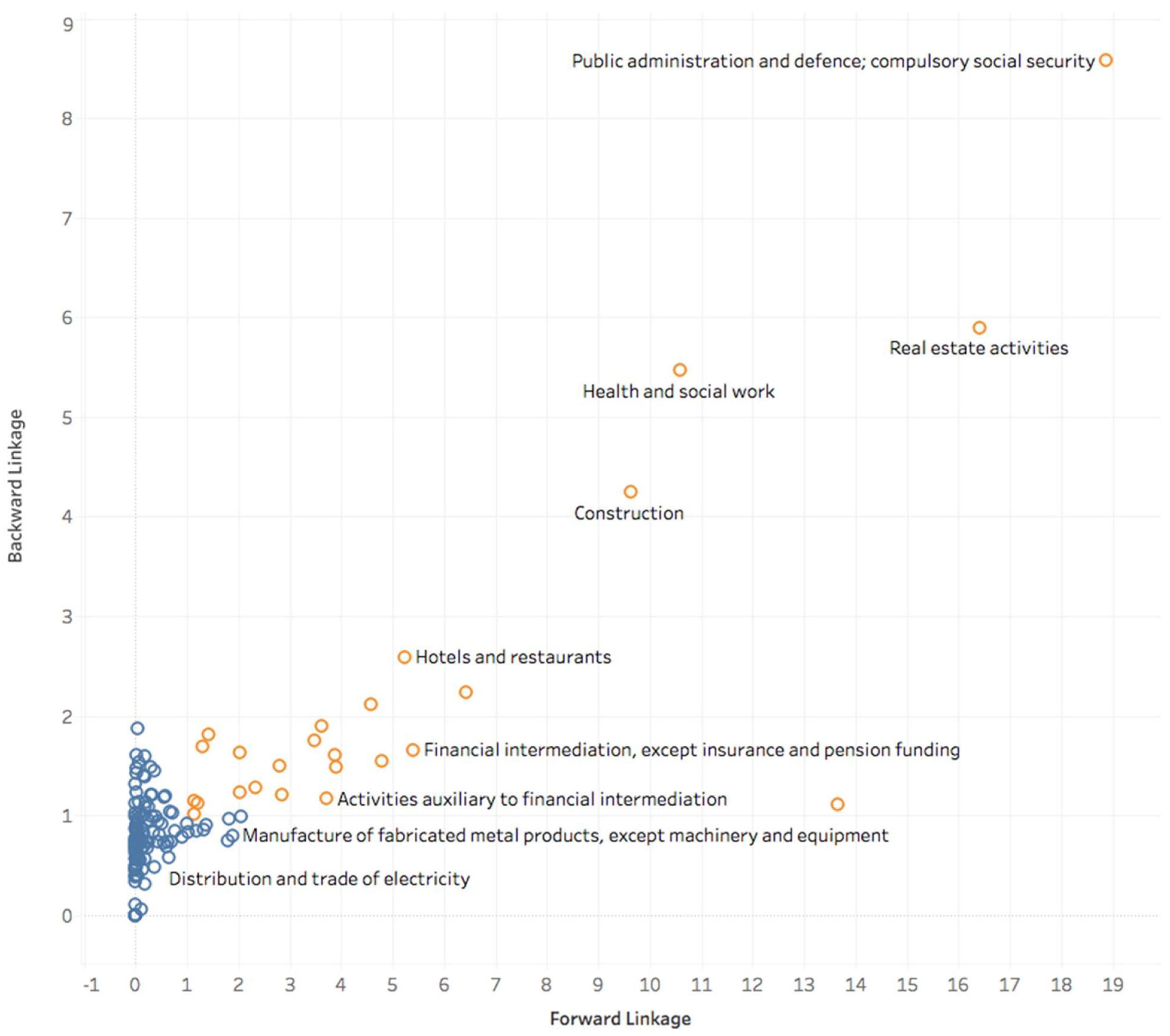
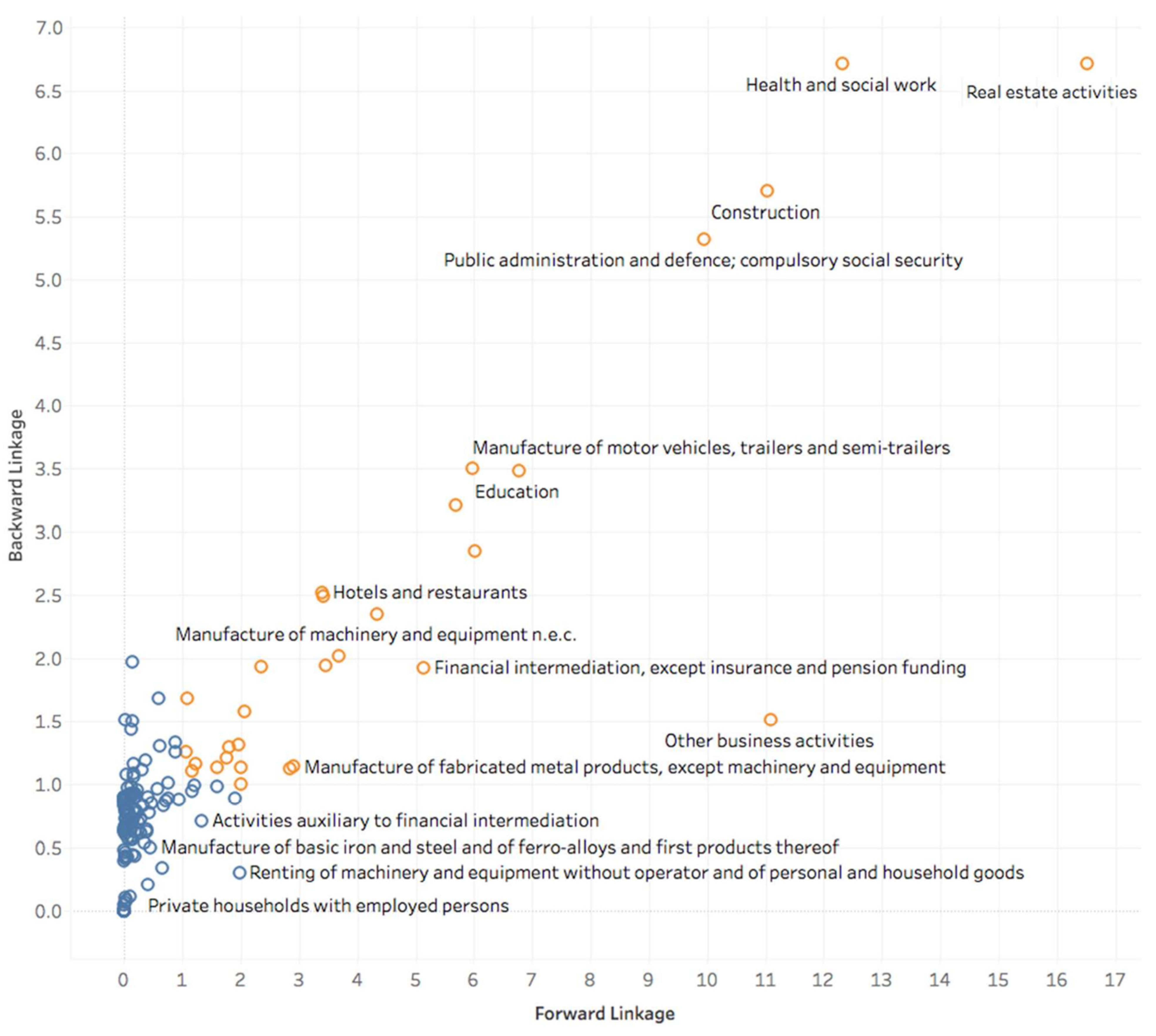
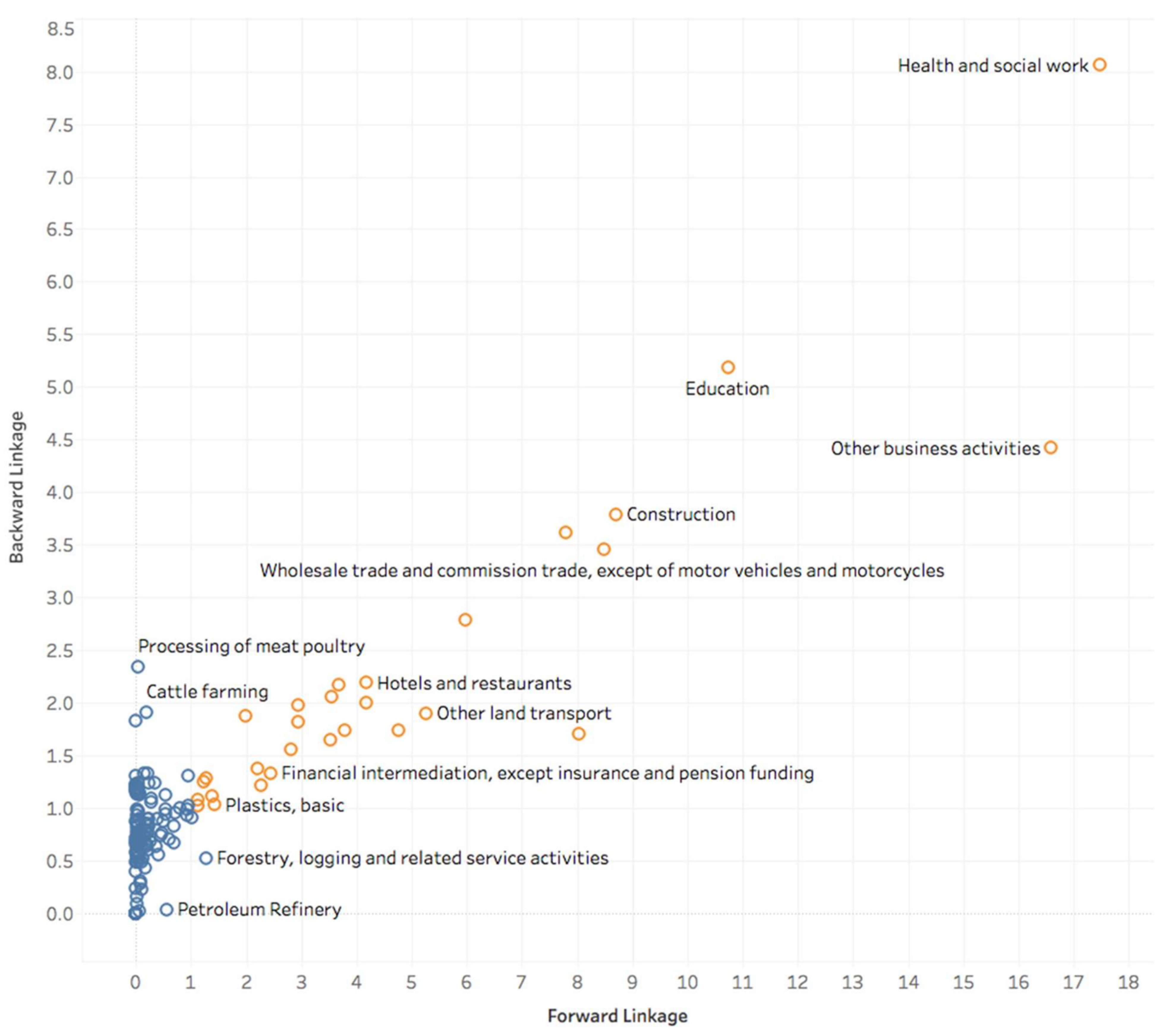
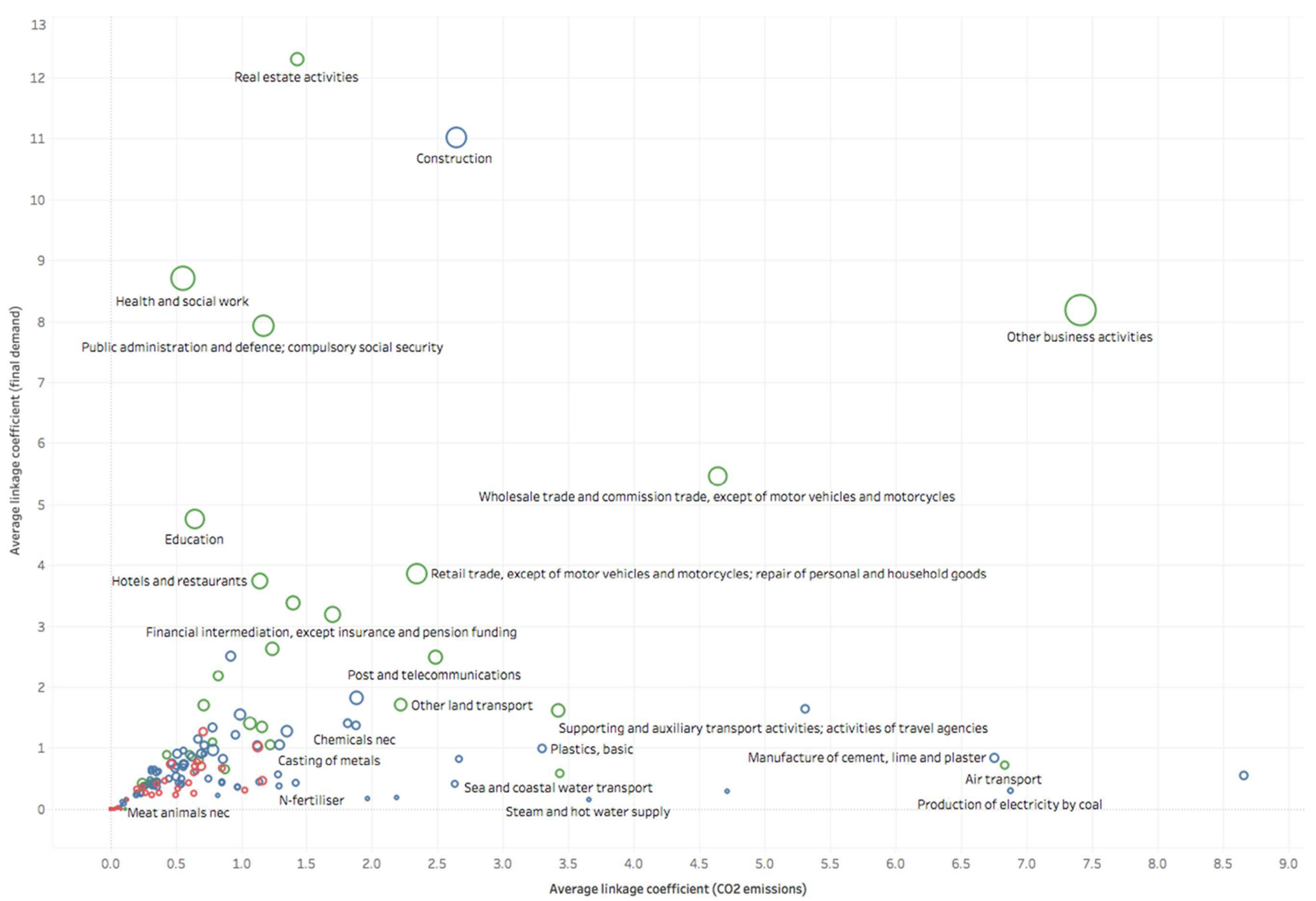
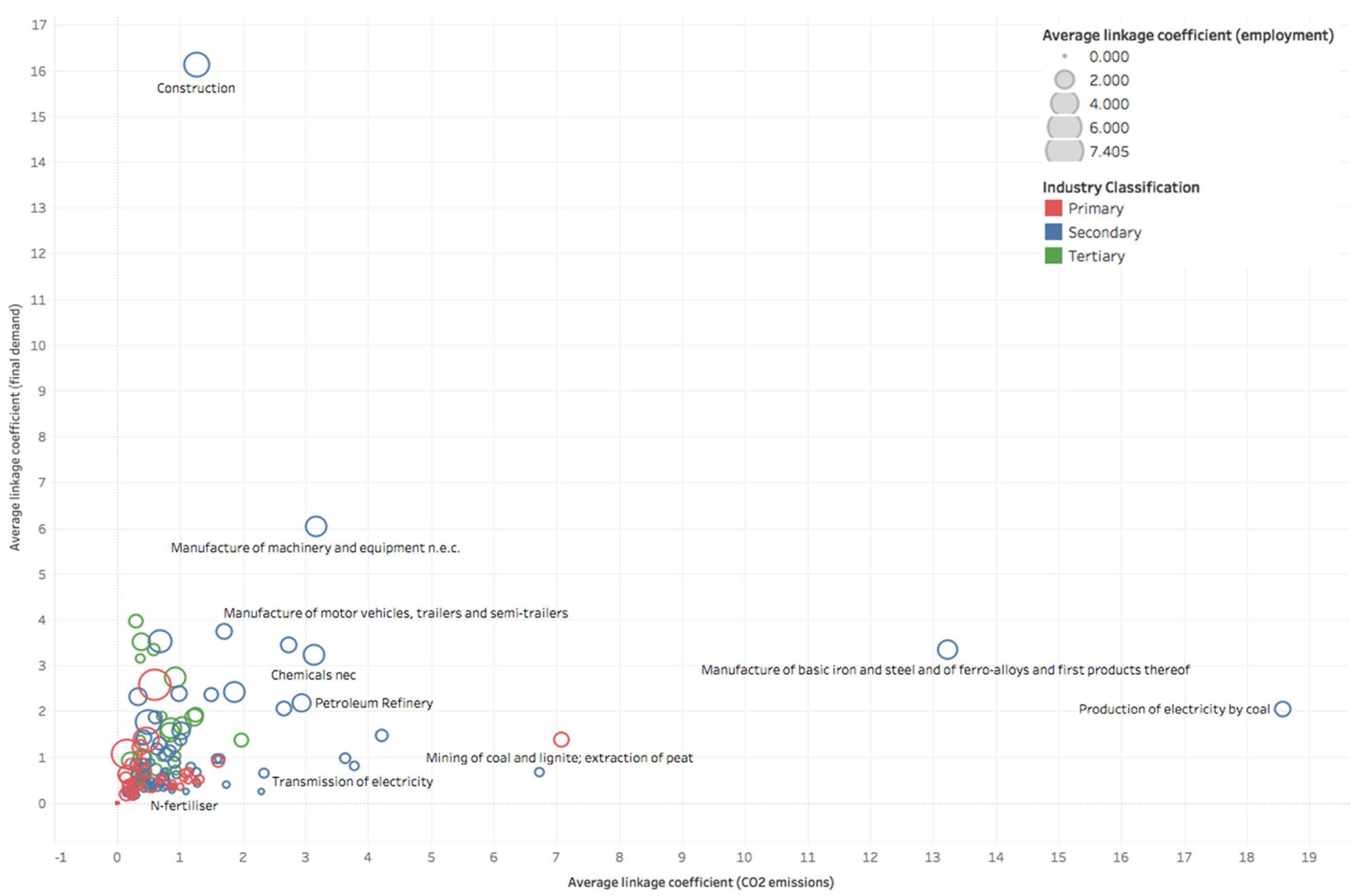
4.1. Forward and Backward Linkage Coefficients


4.2. Sector Sustainability Rankings

5. Discussion
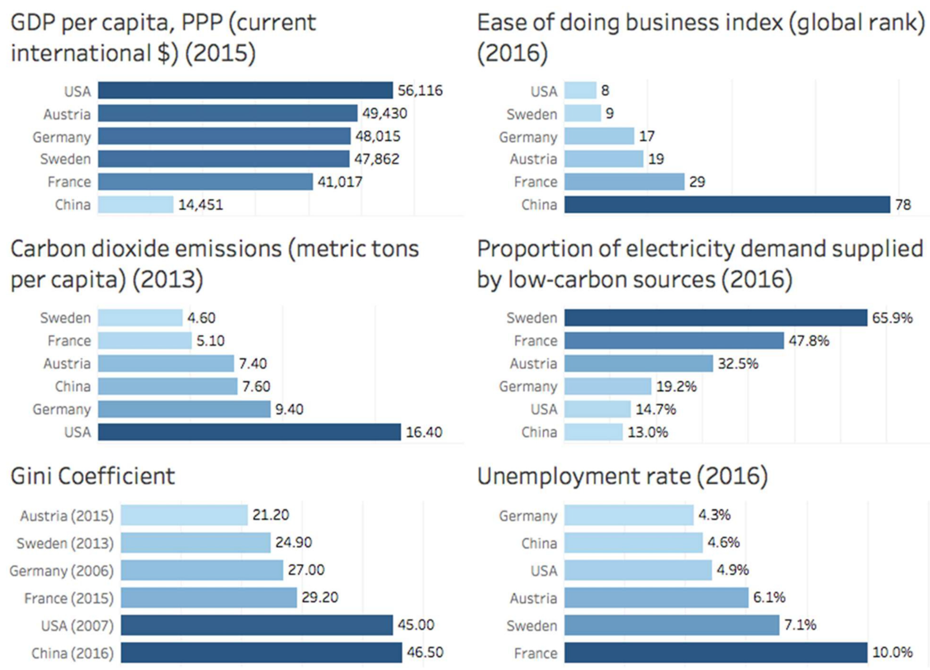
5.1. Differing Economic Structures of the Six Countries

5.2. Policy Implications
6. Conclusions
Author Contributions
Funding
Institutional Review Board Statement
Informed Consent Statement
Data Availability Statement
Conflicts of Interest
Appendix A. Complete Forward and Backward Linkage Coefficients

| Austria | China | |||||||||||
| Final Demand | CO2 | Employment | Final Demand | CO2 | Employment | |||||||
| Sector ID | Fwd | Bckwd | Fwd | Bckwd | Fwd | Bckwd | Fwd | Bckwd | Fwd | Bckwd | Fwd | Bckwd |
| 1 | 0 | 0 | 0 | 0 | 0 | 0 | 0.57 | 0.21 | 0.58 | 0.48 | 2.49 | 1.32 |
| 2 | 0.07 | 0.69 | 0.15 | 0.35 | 0.42 | 0.81 | 0.38 | 0.23 | 0.15 | 0.36 | 1.38 | 0.83 |
| 3 | 0.21 | 0.66 | 0.44 | 0.54 | 0.98 | 0.92 | 0.5 | 0.31 | 0.22 | 0.44 | 1.67 | 1.03 |
| 4 | 0.46 | 0.81 | 0.43 | 0.58 | 1.13 | 1.11 | 3.06 | 2.08 | 0.7 | 0.52 | 9.05 | 5.76 |
| 5 | 0.04 | 0.37 | 0.07 | 0.18 | 0.09 | 0.38 | 0.32 | 0.19 | 0.15 | 0.29 | 1.39 | 0.86 |
| 6 | 0.02 | 0.7 | 0.04 | 0.26 | 0.08 | 0.7 | 0.22 | 0.14 | 0.14 | 0.17 | 1.37 | 0.89 |
| 7 | 0 | 0.02 | 0 | 0 | 0 | 0.02 | 0.09 | 0.25 | 0.06 | 0.43 | 0.74 | 0.66 |
| 8 | 0.22 | 0.8 | 0.08 | 0.34 | 1.25 | 1.13 | 0.71 | 0.54 | 0.13 | 0.21 | 2.92 | 1.88 |
| 9 | 0.11 | 2.17 | 0.15 | 1.07 | 1.21 | 2.91 | 0.23 | 1.46 | 0.19 | 0.54 | 0.82 | 1.66 |
| 10 | 0.25 | 0.85 | 0.07 | 0.38 | 0.79 | 1.29 | 1.36 | 1.41 | 0.54 | 0.38 | 5.31 | 4.01 |
| 11 | 0.15 | 0.71 | 0.01 | 0.34 | 0.27 | 0.85 | 0.65 | 1.78 | 0.21 | 0.52 | 1.35 | 2.17 |
| 12 | 0.08 | 0.07 | 0.02 | 0.02 | 0.04 | 0.06 | 0.15 | 0.93 | 0.03 | 0.26 | 0.8 | 1.25 |
| 13 | 0.08 | 0.07 | 0.01 | 0.02 | 0.04 | 0.06 | 0.24 | 1.44 | 0.04 | 0.41 | 0.5 | 1.61 |
| 14 | 0.32 | 0.52 | 0.16 | 0.24 | 1.3 | 1.07 | 0.29 | 1.11 | 0.16 | 0.74 | 0.7 | 1.37 |
| 15 | 0 | 0.51 | 0 | 0.23 | 0 | 0.58 | 0.01 | 0.78 | 0.01 | 0.32 | 0.06 | 0.78 |
| 16 | 0 | 0 | 0.05 | 0.04 | 0 | 0 | 0 | 0 | 0.01 | 0 | 0 | 0 |
| 17 | 0 | 0 | 0 | 0 | 0 | 0 | 0 | 0 | 0 | 0 | 0 | 0 |
| 18 | 0.67 | 0.55 | 0.45 | 0.33 | 1.43 | 0.85 | 0.42 | 0.28 | 0.28 | 0.14 | 2.21 | 1.43 |
| 19 | 0.01 | 1.16 | 0 | 0.51 | 0.02 | 1.13 | 1.73 | 0.4 | 0.2 | 0.11 | 8.25 | 5.23 |
| 20 | 0 | 0.81 | 0 | 0.36 | 0 | 0.73 | 2.04 | 0.7 | 12.65 | 1.5 | 2.26 | 0.83 |
| 21 | 0.05 | 0.63 | 0.24 | 0.34 | 0.03 | 0.79 | 1.15 | 0.67 | 1.84 | 1.39 | 1.43 | 0.6 |
| 22 | 0.04 | 0.54 | 0.83 | 0.86 | 0.04 | 0.73 | 0.46 | 0.53 | 1.29 | 1.33 | 0.55 | 0.46 |
| 23 | 0 | 0 | 0 | 0 | 0 | 0 | 0 | 0 | 0.02 | 0.01 | 0 | 0 |
| 24 | 0 | 0 | 0 | 0 | 0 | 0 | 0.01 | 0.67 | 0 | 1.83 | 0 | 0.52 |
| 25 | 0.01 | 1.16 | 0.17 | 0.52 | 0.01 | 1.23 | 0.06 | 0.78 | 0.2 | 1.57 | 0.05 | 0.64 |
| 26 | 0 | 0 | 0 | 0 | 0 | 0 | 0.29 | 0.71 | 0.28 | 1.98 | 0.22 | 0.6 |
| 27 | 0 | 0 | 0 | 0 | 0 | 0 | 0.04 | 0.67 | 0.09 | 1.93 | 0.04 | 0.54 |
| 28 | 0 | 0 | 0 | 0 | 0 | 0 | 0.03 | 0.68 | 0.06 | 1.64 | 0.02 | 0.55 |
| 29 | 0 | 0 | 0 | 0 | 0 | 0 | 0.23 | 0.83 | 0.31 | 1.82 | 0.18 | 0.66 |
| 30 | 0 | 0 | 0 | 0 | 0 | 0 | 0.04 | 0.87 | 0.03 | 2.51 | 0.03 | 0.67 |
| 31 | 0.04 | 1.28 | 0.63 | 0.61 | 0.04 | 1.27 | 0.4 | 0.93 | 0.72 | 1.57 | 0.31 | 0.73 |
| 32 | 0.11 | 1.14 | 0.1 | 0.7 | 0.1 | 1.22 | 0.22 | 0.79 | 0.32 | 1.09 | 0.16 | 0.66 |
| 33 | 0.24 | 1.03 | 0.55 | 0.77 | 0.25 | 1 | 0.56 | 0.72 | 1.08 | 1.11 | 0.44 | 0.65 |
| 34 | 0.01 | 1.4 | 0.02 | 0.68 | 0.01 | 1.15 | 0.03 | 1.03 | 0.06 | 1.38 | 0.04 | 0.84 |
| 35 | 0.3 | 1.3 | 0.08 | 0.77 | 0.14 | 1.61 | 0.03 | 1.63 | 0.01 | 0.62 | 0.02 | 1.86 |
| 36 | 0.43 | 1.22 | 0.12 | 0.53 | 0.14 | 1.99 | 0.09 | 3.43 | 0.04 | 0.97 | 0.05 | 9.27 |
| 37 | 0.07 | 0.14 | 0.01 | 0.06 | 0.07 | 0.17 | 0.12 | 2.73 | 0.04 | 0.82 | 0.08 | 3.29 |
| 38 | 0.44 | 0.25 | 0.04 | 0.03 | 1.26 | 0.63 | 0.39 | 0.83 | 0.12 | 0.5 | 0.41 | 0.88 |
| 39 | 0.1 | 0.16 | 0.03 | 0.05 | 0.33 | 0.3 | 0.19 | 0.47 | 0.08 | 0.42 | 0.21 | 0.97 |
| 40 | 0.68 | 1.42 | 0.22 | 0.62 | 0.28 | 1.4 | 0.11 | 1.17 | 0.05 | 0.77 | 0.12 | 1.43 |
| 41 | 0 | 0.04 | 0 | 0.02 | 0 | 0.05 | 0.16 | 0.61 | 0.45 | 1.13 | 0.08 | 1.02 |
| 42 | 0.09 | 0.25 | 0.03 | 0.1 | 0.05 | 0.25 | 0.04 | 0.45 | 0.02 | 0.3 | 0.04 | 1.24 |
| 43 | 1.48 | 1.57 | 1.01 | 1.15 | 0.61 | 1.28 | 4.51 | 2.53 | 0.9 | 0.49 | 5.63 | 2.08 |
| 44 | 0.98 | 1.53 | 0.15 | 0.65 | 0.6 | 1.4 | 0.4 | 1.12 | 0.08 | 0.75 | 0.24 | 1.26 |
| 45 | 0.03 | 1.14 | 0.01 | 0.52 | 0.02 | 1.35 | 2.6 | 2.02 | 0.3 | 0.39 | 1.05 | 3.3 |
| 46 | 0.12 | 0.63 | 0.01 | 0.28 | 0.04 | 0.74 | 0.12 | 0.65 | 0.06 | 0.47 | 0.02 | 1.15 |
| 47 | 0.24 | 0.73 | 0.24 | 0.47 | 0.51 | 0.92 | 2.37 | 0.79 | 1.2 | 0.86 | 2.78 | 1.55 |
| 48 | 0.03 | 0.69 | 0.03 | 0.27 | 0.22 | 0.83 | 1.92 | 1.81 | 0.51 | 0.71 | 1.08 | 1.52 |
| 49 | −0.02 | 0.8 | 0.04 | 0.4 | 0.14 | 1 | 0.78 | 0.9 | 0.35 | 0.56 | 0.73 | 1.19 |
| 50 | 1.36 | 1.14 | 0.91 | 0.81 | 1.57 | 1.37 | 0.12 | 0.23 | 0.12 | 0.48 | 0.11 | 0.52 |
| 51 | 0.26 | 0.97 | 0.12 | 0.52 | 0.34 | 1.07 | 0.01 | 0.21 | 0.01 | 0.51 | 0.01 | 0.23 |
| 52 | 0.15 | 0.79 | 0.2 | 0.81 | 0.42 | 1 | 0.01 | 0.66 | 0.03 | 1.44 | 0.01 | 0.73 |
| 53 | 0.06 | 0.79 | 0.71 | 1.08 | 0.2 | 0.94 | 0.01 | 0.69 | 0.04 | 1.1 | 0.01 | 0.64 |
| 54 | 0.39 | 0.88 | 0.23 | 0.57 | 0.39 | 1.05 | 1.1 | 0.64 | 0.84 | 0.97 | 1.27 | 0.86 |
| 55 | 1.44 | 0.98 | 1.97 | 1.47 | 2.07 | 1.22 | 1.42 | 0.7 | 0.79 | 0.78 | 1.82 | 0.97 |
| 56 | 0.05 | 0.62 | 2.61 | 2.17 | 0.03 | 0.72 | 0.46 | 0.82 | 2.94 | 1.74 | 0.47 | 0.76 |
| 57 | 0.97 | 0.72 | 4.31 | 3.13 | 0.45 | 0.49 | 3.81 | 0.55 | 4.97 | 0.91 | 4.17 | 0.63 |
| 58 | 0 | 0.69 | 0 | 0.25 | 0 | 0.78 | 0 | 1.75 | 0 | 1.06 | 0 | 0.92 |
| 59 | 0.77 | 0.8 | 1.09 | 1.03 | 1.01 | 0.95 | 0.51 | 0.66 | 0.49 | 1.02 | 0.6 | 0.74 |
| 60 | 0.02 | 0.55 | 0.01 | 0.31 | 0.02 | 0.65 | 0.04 | 0.73 | 0.03 | 0.98 | 0.05 | 0.77 |
| 61 | 0 | 0.57 | 1.92 | 1.96 | 0.01 | 0.61 | 0 | 0.48 | 1.01 | 1.18 | 0.01 | 0.49 |
| 62 | 0 | 0.57 | 0.03 | 0.44 | 0.01 | 0.61 | 0.54 | 0.49 | 0.54 | 0.92 | 1.93 | 0.55 |
| 63 | 0.13 | 0.94 | 0.85 | 1.24 | 0.17 | 0.95 | 5.38 | 1.09 | 4.66 | 1.63 | 5.06 | 1.02 |
| 64 | 0.69 | 0.92 | 0.45 | 0.51 | 1.26 | 1.25 | 3.99 | 0.86 | 2.55 | 1.19 | 4.46 | 1.64 |
| 65 | 0.04 | 0.67 | 0.17 | 0.48 | 0.04 | 0.75 | 1.59 | 0.67 | 0.73 | 0.97 | 1.16 | 0.77 |
| 66 | 0.01 | 0.66 | 0.13 | 0.46 | 0.01 | 0.73 | 0 | 0 | 0 | 0 | 0 | 0 |
| 67 | 0.05 | 0.7 | 0.04 | 0.39 | 0.07 | 0.74 | 1.67 | 0.69 | 0.15 | 1.13 | 0.99 | 0.92 |
| 68 | 0.11 | 0.81 | 0.98 | 1.21 | 0.1 | 0.81 | 0.05 | 0.65 | 0.43 | 1.35 | 0.02 | 0.61 |
| 69 | 1.48 | 0.98 | 5.97 | 4.83 | 1.63 | 1.28 | 0.68 | 0.66 | 8.54 | 4.91 | 0.3 | 0.72 |
| 70 | 0.05 | 0.88 | 1.67 | 2.32 | 0.05 | 0.97 | 0.12 | 0.65 | 1.54 | 1.94 | 0.05 | 0.67 |
| 71 | 0.15 | 0.76 | 0.42 | 0.69 | 0.17 | 0.8 | 1.17 | 0.73 | 1.35 | 1.83 | 0.75 | 0.77 |
| 72 | 0.07 | 0.45 | 10.32 | 8.7 | 0.39 | 0.64 | 6.11 | 0.59 | 19.81 | 6.65 | 4.39 | 1.14 |
| 73 | 0.04 | 0.49 | 5.4 | 4.81 | 0.25 | 0.61 | 1.34 | 0.6 | 3.6 | 3.67 | 0.99 | 0.77 |
| 74 | 0.02 | 0.45 | 0.08 | 0.22 | 0.03 | 0.51 | 0.45 | 0.75 | 0.53 | 1.37 | 0.28 | 0.59 |
| 75 | 0 | 0 | 0 | 0 | 0 | 0 | 0 | 0 | 0 | 0 | 0 | 0 |
| 76 | 0.21 | 0.62 | 1.46 | 1.64 | 0.29 | 0.75 | 1.22 | 0.7 | 1.22 | 2.05 | 0.87 | 0.64 |
| 77 | 0.01 | 0.62 | 0.07 | 0.71 | 0.02 | 0.77 | 0.03 | 0.7 | 0.03 | 1.09 | 0.03 | 0.57 |
| 78 | 0 | 0.41 | 0.08 | 0.57 | 0 | 0.49 | 0.32 | 0.53 | 0.23 | 0.99 | 0.17 | 0.44 |
| 79 | 0 | 0.42 | 0.04 | 0.56 | 0 | 0.5 | 0.03 | 0.53 | 0.02 | 0.84 | 0.02 | 0.42 |
| 80 | 0.14 | 0.52 | 0.14 | 0.41 | 0.18 | 0.61 | 0.8 | 0.49 | 0.52 | 0.99 | 0.43 | 0.43 |
| 81 | 0.02 | 0.51 | 0.03 | 0.42 | 0.03 | 0.58 | 0.11 | 0.48 | 0.12 | 1.03 | 0.06 | 0.4 |
| 82 | 0.13 | 0.82 | 4.23 | 3.57 | 0.15 | 0.8 | 0.68 | 0.88 | 0.93 | 1.41 | 0.42 | 0.67 |
| 83 | 0 | 0 | 0 | 0 | 0 | 0 | 0 | 0 | 0 | 0 | 0 | 0 |
| 84 | 0.41 | 0.56 | 2.17 | 1.35 | 0.43 | 0.65 | 0.56 | 0.78 | 0.66 | 1.86 | 0.36 | 0.73 |
| 85 | 2.78 | 1.46 | 1.12 | 0.62 | 3.31 | 1.76 | 3.04 | 1.06 | 2.62 | 2.69 | 2.28 | 1.14 |
| 86 | 2.62 | 1.64 | 1.29 | 0.66 | 3.27 | 1.97 | 8.01 | 4.06 | 4.51 | 1.85 | 4.39 | 1.84 |
| 87 | 0.03 | 0.85 | 0 | 0.31 | 0.04 | 0.89 | 1.58 | 1.19 | 1.35 | 0.68 | 1.21 | 0.91 |
| 88 | 1.38 | 1.09 | 1.08 | 0.68 | 1.61 | 1.32 | 4.69 | 2.2 | 3.76 | 1.72 | 2.48 | 1.18 |
| 89 | 0.55 | 0.88 | 0.14 | 0.41 | 0.71 | 1.03 | 1.52 | 1.07 | 0.62 | 0.75 | 1.42 | 1.06 |
| 90 | 0.55 | 0.85 | 0.16 | 0.32 | 0.82 | 1.1 | 0.43 | 0.77 | 0.2 | 0.73 | 0.44 | 0.73 |
| 91 | 1.23 | 1.02 | 0.31 | 0.37 | 1.15 | 1.04 | 4.12 | 3.36 | 1.79 | 1.62 | 2.28 | 1.65 |
| 92 | 0.62 | 0.81 | 0.3 | 0.36 | 0.48 | 0.85 | 2.49 | 2.23 | 1.12 | 1.87 | 1.74 | 1.15 |
| 93 | 1.14 | 1.19 | 0.33 | 0.49 | 1.39 | 1.4 | 2.96 | 1.81 | 1.06 | 0.93 | 2.18 | 1.77 |
| 94 | 0.06 | 0.72 | 0.79 | 0.59 | 0.12 | 0.79 | 0.78 | 0.07 | 1.26 | 0.15 | 0.62 | 0.1 |
| 95 | 0 | 0 | 0.03 | 0.02 | 0 | 0 | 0 | 0 | 0 | 0 | 0 | 0 |
| 96 | 0.11 | 0.68 | 7.29 | 8.02 | 0.11 | 0.61 | 3.21 | 0.87 | 27.36 | 9.79 | 2.76 | 0.75 |
| 97 | 0.35 | 0.46 | 11.04 | 10.03 | 0.23 | 0.33 | 0.05 | 0.5 | 0.57 | 1.19 | 0.04 | 0.41 |
| 98 | 0 | 0 | 0 | 0 | 0 | 0 | 0.07 | 0.33 | 0.08 | 0.2 | 0.06 | 0.25 |
| 99 | 0.51 | 0.68 | 2.83 | 2.13 | 0.48 | 0.61 | 0.57 | 0.44 | 0.64 | 0.3 | 0.47 | 0.31 |
| 100 | 0.02 | 0.68 | 0.05 | 2.23 | 0.02 | 0.56 | 0.01 | 0.4 | 0.01 | 0.28 | 0.01 | 0.28 |
| 101 | 0.06 | 0.62 | 1.25 | 4.58 | 0.04 | 0.42 | 0.06 | 0.59 | 0.33 | 0.96 | 0.04 | 0.49 |
| 102 | 0.17 | 0.75 | 1.46 | 5.3 | 0.12 | 0.48 | 0 | 0.87 | 0 | 0.54 | 0 | 0.63 |
| 103 | 0 | 0.72 | 0 | 2.37 | 0 | 0.6 | 0 | 0.53 | 0 | 0.33 | 0 | 0.36 |
| 104 | 0 | 0 | 0 | 0 | 0 | 0 | 0 | 0 | 0 | 0 | 0 | 0 |
| 105 | 0 | 0 | 0 | 0 | 0 | 0 | 0 | 0 | 0 | 0 | 0 | 0 |
| 106 | 0 | 0.72 | 0 | 4.97 | 0 | 0.44 | 0 | 0.54 | 0 | 0.36 | 0 | 0.37 |
| 107 | 0.02 | 0.49 | 0.11 | 1.91 | 0.02 | 0.4 | 0.02 | 0.5 | 0.02 | 0.55 | 0.02 | 0.37 |
| 108 | 1.43 | 1.04 | 4.27 | 1.35 | 0.93 | 0.65 | 0.66 | 0.94 | 0.74 | 6.81 | 0.51 | 0.7 |
| 109 | 3.53 | 1.38 | 5.82 | 1.36 | 2.1 | 0.72 | 1.85 | 1.09 | 1.6 | 6.83 | 1.28 | 0.7 |
| 110 | 1.58 | 0.91 | 19.23 | 6.8 | 0.87 | 0.51 | 0.24 | 0.63 | 0.31 | 1.08 | 0.15 | 0.49 |
| 111 | 0.21 | 0.77 | 4.58 | 8.73 | 0.11 | 0.46 | 0.08 | 0.39 | 3.09 | 1.5 | 0.09 | 0.36 |
| 112 | 0.24 | 0.92 | 0.13 | 0.47 | 0.28 | 0.88 | 0.19 | 0.66 | 0.19 | 2.36 | 0.12 | 0.49 |
| 113 | 17.65 | 7.35 | 5.1 | 2.71 | 11.02 | 4.55 | 18.15 | 14.09 | 0.8 | 1.75 | 5.31 | 4.05 |
| 114 | 0.03 | 0.11 | 0.08 | 0.12 | 0.03 | 0.12 | 0 | 0 | 0 | 0 | 0 | 0 |
| 115 | 2.45 | 1.66 | 0.58 | 0.4 | 2.85 | 1.74 | 0.78 | 1.24 | 0.26 | 0.57 | 1.29 | 1.39 |
| 116 | 0.2 | 1.47 | 0.14 | 0.42 | 0.21 | 1.63 | 0.05 | 0.97 | 0.05 | 0.59 | 0.06 | 0.61 |
| 117 | 8.3 | 3.38 | 4.21 | 1.02 | 8.7 | 3.34 | 2.4 | 0.97 | 1.82 | 0.25 | 3.04 | 1.44 |
| 118 | 5.52 | 3.04 | 2.44 | 0.7 | 10.26 | 4.8 | 1.83 | 1.26 | 1.14 | 0.56 | 3.36 | 2.09 |
| 119 | 7.41 | 4.13 | 1.05 | 0.48 | 7.35 | 3.78 | 3.3 | 2.18 | 1.3 | 0.55 | 3.5 | 2.59 |
| 120 | 0.97 | 1.11 | 0.65 | 0.63 | 0.52 | 0.85 | 0.6 | 0.71 | 0.85 | 0.7 | 0.49 | 0.56 |
| 121 | 2.42 | 1.49 | 2.66 | 1.41 | 4.12 | 2.18 | 1.64 | 0.87 | 1.09 | 0.72 | 1.96 | 1.17 |
| 122 | 0.09 | 2.32 | 0.89 | 1.49 | 0.19 | 1.99 | 0.07 | 1.92 | 0.29 | 1.13 | 0.09 | 0.97 |
| 123 | 0.01 | 1.18 | 0.04 | 0.46 | 0 | 0.91 | 0.58 | 0.83 | 1.12 | 0.76 | 0.62 | 0.68 |
| 124 | 0.01 | 1.06 | 0.07 | 0.61 | 0.02 | 1.28 | 0.04 | 0.9 | 0.36 | 0.74 | 0.04 | 0.65 |
| 125 | 1.08 | 1.48 | 5.88 | 5.12 | 0.66 | 1.15 | 0.69 | 1.34 | 0.79 | 1.08 | 0.66 | 1.11 |
| 126 | 3.51 | 2.76 | 3.59 | 1.44 | 3.24 | 2.3 | 2.66 | 1.08 | 1.99 | 0.46 | 2.89 | 1.26 |
| 127 | 3.38 | 1.73 | 1.71 | 0.98 | 3.27 | 1.64 | 0.15 | 1.12 | 0.19 | 0.56 | 0.34 | 0.75 |
| 128 | 4.33 | 1.46 | 1.8 | 0.3 | 4.88 | 1.84 | 2.28 | 0.44 | 3.77 | 0.18 | 2.39 | 0.34 |
| 129 | 2.54 | 1.7 | 0.39 | 0.3 | 1.27 | 1.28 | 1.45 | 1.28 | 0.46 | 0.29 | 0.81 | 0.5 |
| 130 | 1.08 | 0.85 | 0.32 | 0.3 | 1.44 | 1.26 | 0.57 | 0.67 | 0.41 | 0.24 | 0.47 | 0.5 |
| 131 | 15.44 | 6.9 | 1.92 | 0.59 | 5.93 | 1.66 | 3.69 | 2.62 | 0.54 | 0.2 | 0.9 | 0.3 |
| 132 | 1.71 | 0.8 | 0.89 | 0.33 | 1.56 | 0.7 | 0.33 | 0.96 | 0.28 | 0.66 | 0.24 | 0.75 |
| 133 | 2.32 | 1.69 | 0.42 | 0.32 | 2.11 | 1.54 | 2.34 | 1.43 | 1 | 0.44 | 1.05 | 0.44 |
| 134 | 0.08 | 1.02 | 0.16 | 0.41 | 0.38 | 1.41 | 0.3 | 0.75 | 0.18 | 0.6 | 0.22 | 0.62 |
| 135 | 9.26 | 1.86 | 4.95 | 0.76 | 17.23 | 5.59 | 2.64 | 1.2 | 1.89 | 0.62 | 2.27 | 0.81 |
| 136 | 10.38 | 5.95 | 0.41 | 0.48 | 6.84 | 3.78 | 4.09 | 3.84 | 0.13 | 0.46 | 1.43 | 1.51 |
| 137 | 7.64 | 4.11 | 0.31 | 0.29 | 6.59 | 3.33 | 3.8 | 3.23 | 0.26 | 0.52 | 2.3 | 1.85 |
| 138 | 11.15 | 6.12 | 0.37 | 0.47 | 10.39 | 5.39 | 3.31 | 3.37 | 0.34 | 0.82 | 0.83 | 1.14 |
| 139 | 0.07 | 0.81 | 0.08 | 0.4 | 0.09 | 0.78 | 0.03 | 0.86 | 0.02 | 0.65 | 0.09 | 0.69 |
| 140 | 0.1 | 0.8 | 0.09 | 0.4 | 0.12 | 0.78 | 0.03 | 0.86 | 0.02 | 0.65 | 0.09 | 0.69 |
| 141 | 0.17 | 0.79 | 0.13 | 0.4 | 0.21 | 0.79 | 0.01 | 0.85 | 0.01 | 0.64 | 0.02 | 0.65 |
| 142 | 0.52 | 0.83 | 0.33 | 0.43 | 0.63 | 0.88 | 0 | 0.85 | 0 | 0.64 | 0.01 | 0.64 |
| 143 | 0.02 | 0.79 | 0.05 | 0.4 | 0.02 | 0.76 | 0.01 | 0.85 | 0.01 | 0.64 | 0.02 | 0.65 |
| 144 | 0.03 | 0.8 | 0.05 | 0.4 | 0.04 | 0.77 | 0.01 | 0.85 | 0.01 | 0.64 | 0.02 | 0.65 |
| 145 | 0.1 | 0.8 | 0.09 | 0.4 | 0.13 | 0.79 | 0.01 | 0.85 | 0.01 | 0.65 | 0.02 | 0.65 |
| 146 | 0.01 | 0.8 | 0.04 | 0.39 | 0.02 | 0.77 | 0 | 0 | 0 | 0 | 0 | 0 |
| 147 | 0 | 0.8 | 0.04 | 0.39 | 0 | 0.77 | 0 | 0 | 0 | 0 | 0 | 0 |
| 148 | 0.01 | 0.8 | 0.04 | 0.39 | 0.01 | 0.77 | 0 | 0 | 0 | 0 | 0 | 0 |
| 149 | 0.42 | 0.82 | 0.28 | 0.45 | 0.51 | 0.85 | 0.01 | 0.84 | 0.01 | 0.86 | 0.02 | 0.65 |
| 150 | 0 | 0.79 | 0.04 | 0.4 | 0 | 0.76 | 0 | 0.85 | 0 | 0.64 | 0 | 0.64 |
| 151 | 0.03 | 0.81 | 0.1 | 0.44 | 0.04 | 0.78 | 0.09 | 0.89 | 0.09 | 0.66 | 0.32 | 0.83 |
| 152 | 0.07 | 0.81 | 0.12 | 0.44 | 0.08 | 0.78 | 0.17 | 0.93 | 0.16 | 0.67 | 0.57 | 0.98 |
| 153 | 0.01 | 0.8 | 0.04 | 0.39 | 0.01 | 0.77 | 0.08 | 0.89 | 0.08 | 0.48 | 0.29 | 0.81 |
| 154 | 0.01 | 0.81 | 0.04 | 0.39 | 0.02 | 0.77 | 0.03 | 0.86 | 0.03 | 0.47 | 0.12 | 0.71 |
| 155 | 0 | 0.81 | 0.04 | 0.38 | 0 | 0.77 | 0.03 | 0.86 | 0.03 | 0.47 | 0.1 | 0.7 |
| 156 | 0.03 | 0.81 | 0.06 | 0.39 | 0.04 | 0.78 | 0.03 | 0.86 | 0.03 | 0.47 | 0.1 | 0.7 |
| 157 | 0 | 0.81 | 0.04 | 0.38 | 0 | 0.77 | 0.01 | 0.85 | 0.01 | 0.46 | 0.04 | 0.66 |
| 158 | 0.01 | 0.81 | 0.04 | 0.38 | 0.01 | 0.77 | 0.01 | 0.86 | 0.01 | 0.46 | 0.05 | 0.67 |
| 159 | 1.56 | 1.65 | 0.28 | 0.57 | 1.29 | 1.55 | 0.58 | 1.23 | 0.04 | 0.4 | 2.13 | 2.19 |
| 160 | 2.91 | 2.03 | 0.62 | 0.55 | 2.8 | 1.88 | 0.79 | 1.19 | 0.31 | 0.51 | 2.59 | 2.2 |
| 161 | 1.29 | 1.41 | 0.15 | 0.32 | 1.67 | 1.34 | 1.79 | 1.44 | 1.21 | 0.52 | 3.84 | 2.44 |
| 162 | 0.04 | 0.02 | 0.04 | 0.04 | 0.26 | 0.13 | 0.24 | 1.19 | 0.04 | 1.19 | 0.85 | 1.21 |
| 163 | 0 | 0 | 0.04 | 0.03 | 0 | 0 | 0 | 0 | 0 | 0 | 0 | 0 |
| France | Germany | |||||||||||
| Final Demand | CO2 | Employment | Final Demand | CO2 | Employment | |||||||
| Sector ID | Fwd | Bckwd | Fwd | Bckwd | Fwd | Bckwd | Fwd | Bckwd | Fwd | Bckwd | Fwd | Bckwd |
| 1 | 0 | 0.03 | 0.04 | 0.06 | 0 | 0.03 | 0 | 0 | 0 | 0 | 0 | 0 |
| 2 | 0.27 | 0.66 | 1.02 | 1.3 | 0.7 | 0.89 | 0.15 | 0.73 | 0.03 | 0.44 | 0.22 | 0.88 |
| 3 | 0.21 | 0.39 | 0.99 | 1.06 | 0.36 | 0.47 | 0.14 | 0.71 | 0.1 | 0.53 | 0.25 | 0.89 |
| 4 | 1.15 | 0.89 | 1.14 | 1.12 | 1.71 | 1.04 | 0.28 | 0.61 | 0.04 | 0.41 | 0.54 | 0.8 |
| 5 | 0.11 | 0.41 | 0.52 | 0.75 | 0.3 | 0.5 | 0.06 | 0.57 | 0.01 | 0.37 | 0.28 | 0.75 |
| 6 | 0.05 | 0.47 | 0.18 | 0.56 | 0.16 | 0.52 | 0.03 | 0.7 | 0.01 | 0.42 | 0.08 | 0.86 |
| 7 | 0.01 | 0.03 | 0.04 | 0.05 | 0 | 0.03 | 0 | 0 | 0 | 0 | 0 | 0 |
| 8 | 0.23 | 0.24 | 0.32 | 0.32 | 0.24 | 0.26 | 0.15 | 1.06 | 0.05 | 0.72 | 0.4 | 1.21 |
| 9 | 0.27 | 1.07 | 0.44 | 1.26 | 0.13 | 1.13 | 0.12 | 1.44 | 0.01 | 1.12 | 0.25 | 2.04 |
| 10 | 0.12 | 1.08 | 0.1 | 1.17 | 0.09 | 1.18 | 0.3 | 1.11 | 0.06 | 0.9 | 0.22 | 1.49 |
| 11 | 0.24 | 1.16 | 0.09 | 1.2 | 0.08 | 1.18 | 0.14 | 0.56 | 0.01 | 0.5 | 0.12 | 0.59 |
| 12 | 0.12 | 0.17 | 0.08 | 0.18 | 0.06 | 0.17 | 0.04 | 0.08 | 0.02 | 0.05 | 0.03 | 0.08 |
| 13 | 0.01 | 0.05 | 0.04 | 0.08 | 0 | 0.05 | 0.02 | 0.06 | 0.01 | 0.03 | 0.02 | 0.05 |
| 14 | 0.41 | 0.99 | 0.37 | 1.01 | 0.81 | 1.23 | 0.39 | 0.62 | 0.07 | 0.42 | 0.34 | 0.78 |
| 15 | 0 | 0.54 | 0.04 | 0.49 | 0 | 0.57 | 0 | 0.62 | 0 | 0.48 | 0 | 1.01 |
| 16 | 0 | 0 | 0.09 | 0.07 | 0 | 0 | 0 | 0 | 0.01 | 0.01 | 0 | 0 |
| 17 | 0 | 0 | 0.04 | 0.03 | 0 | 0 | 0 | 0 | 0 | 0 | 0 | 0 |
| 18 | 0.36 | 0.44 | 0.26 | 0.45 | 0.3 | 0.46 | 0.14 | 0.44 | 0.05 | 0.24 | 0.2 | 0.56 |
| 19 | 0.09 | 0.38 | 0.27 | 0.73 | 0.13 | 0.46 | 0.02 | 0.43 | 0.02 | 1.02 | 0.02 | 0.41 |
| 20 | 0 | 1.47 | 0.08 | 0.85 | 0 | 2.38 | 0.14 | 1.5 | 4.39 | 1.92 | 0.21 | 1.33 |
| 21 | 0.02 | 0.68 | 0.07 | 0.42 | 0.01 | 0.83 | 0.02 | 0.67 | 0.05 | 0.6 | 0.01 | 0.93 |
| 22 | 0 | 0.63 | 0 | 0.4 | 0 | 0.82 | 0.11 | 0.69 | 0.06 | 0.61 | 0.02 | 0.9 |
| 23 | 0 | 0 | 0 | 0 | 0 | 0 | 0 | 0.48 | 0 | 0.38 | 0 | 0.99 |
| 24 | 0 | 0 | 0 | 0 | 0 | 0 | 0 | 0.83 | 0 | 0.78 | 0 | 1 |
| 25 | 0 | 0 | 0 | 0 | 0 | 0 | 0 | 0.88 | 0 | 0.81 | 0 | 0.96 |
| 26 | 0 | 0 | 0 | 0 | 0 | 0 | 0 | 0 | 0 | 0 | 0 | 0 |
| 27 | 0 | 0 | 0 | 0 | 0 | 0 | 0 | 0 | 0 | 0 | 0 | 0 |
| 28 | 0 | 1.54 | 0 | 1.33 | 0 | 1.42 | 0 | 0 | 0 | 0 | 0 | 0 |
| 29 | 0 | 0 | 0.02 | 0.02 | 0 | 0 | 0 | 0 | 0 | 0 | 0 | 0 |
| 30 | 0 | 0 | 0 | 0 | 0 | 0 | 0 | 0.84 | 0.01 | 0.84 | 0 | 0.91 |
| 31 | 0 | 2.53 | 0 | 1.42 | 0 | 1.88 | 0 | 0.88 | 0 | 0.79 | 0 | 0.9 |
| 32 | 0.19 | 0.67 | 0.57 | 0.63 | 0.22 | 0.75 | 0.08 | 0.69 | 0.13 | 0.7 | 0.09 | 0.96 |
| 33 | 0.07 | 0.61 | 0.35 | 0.68 | 0.09 | 0.63 | 0.09 | 0.64 | 0.27 | 0.8 | 0.12 | 0.75 |
| 34 | 0.02 | 0.9 | 0.05 | 0.78 | 0.01 | 0.93 | 0.02 | 0.89 | 0.05 | 0.81 | 0.02 | 0.88 |
| 35 | 0.44 | 1.27 | 0.13 | 1.11 | 0.22 | 1.35 | 0.15 | 1.09 | 0.02 | 0.78 | 0.09 | 2.03 |
| 36 | 0.32 | 1.61 | 0.14 | 1.43 | 0.14 | 2.98 | 0.58 | 1.68 | 0.15 | 0.86 | 0.22 | 1.24 |
| 37 | 0.31 | 1.51 | 0.09 | 1.3 | 0.06 | 1.96 | 0.1 | 0.11 | 0.02 | 0.06 | 0.02 | 0.08 |
| 38 | 0.61 | 1.69 | 0.07 | 1.27 | 0.05 | 1.5 | 0.64 | 0.34 | 0.03 | 0.04 | 1.53 | 0.61 |
| 39 | 0.07 | 0.09 | 0.09 | 0.12 | 0.25 | 0.17 | 0.2 | 0.77 | 0.03 | 0.37 | 0.26 | 0.87 |
| 40 | 0.94 | 1.47 | 0.58 | 1.33 | 0.5 | 1.38 | 0.87 | 1.26 | 0.14 | 0.83 | 0.26 | 0.96 |
| 41 | 0.01 | 0.02 | 0.06 | 0.06 | 0.03 | 0.04 | 0 | 0.04 | 0 | 0.02 | 0.01 | 0.05 |
| 42 | 0.22 | 0.3 | 0.15 | 0.31 | 0.56 | 0.55 | 0.17 | 0.43 | 0.02 | 0.24 | 0.28 | 0.52 |
| 43 | 1.56 | 1.24 | 1.79 | 1.83 | 0.76 | 1.03 | 2.34 | 1.93 | 0.75 | 1.21 | 0.49 | 1.57 |
| 44 | 1.23 | 1.43 | 0.47 | 1.1 | 0.95 | 1.44 | 0.87 | 1.33 | 0.14 | 0.92 | 0.33 | 0.99 |
| 45 | 0.21 | 1.16 | 0.1 | 1.02 | 0.11 | 1.27 | 0.12 | 0.98 | 0.02 | 0.63 | 0.03 | 0.93 |
| 46 | 0.04 | 0.47 | 0.06 | 0.35 | 0.01 | 0.62 | 0.16 | 0.8 | 0.01 | 0.46 | 0.03 | 1.03 |
| 47 | 0.27 | 0.8 | 0.3 | 0.71 | 0.44 | 1.06 | 0.27 | 0.73 | 0.13 | 0.67 | 0.38 | 0.78 |
| 48 | 0.26 | 0.95 | 0.05 | 0.65 | 0.23 | 1.17 | 0.41 | 0.9 | 0.03 | 0.47 | 0.16 | 0.77 |
| 49 | 0 | 0.72 | 0.03 | 0.69 | 0.11 | 0.9 | 0.06 | 0.69 | 0.03 | 0.5 | 0.08 | 0.72 |
| 50 | 0.46 | 0.86 | 0.32 | 0.67 | 0.69 | 1.07 | 0.72 | 0.87 | 0.32 | 0.66 | 0.89 | 0.92 |
| 51 | 0.04 | 0.81 | 0.04 | 0.64 | 0.07 | 0.97 | 0.04 | 0.79 | 0.02 | 0.63 | 0.05 | 0.78 |
| 52 | 0.11 | 0.88 | 0.14 | 0.75 | 0.21 | 1.15 | 0.1 | 0.7 | 0.12 | 0.98 | 0.24 | 0.81 |
| 53 | 0.08 | 0.9 | 0.27 | 0.81 | 0.17 | 1.23 | 0.06 | 0.75 | 0.23 | 0.84 | 0.18 | 0.89 |
| 54 | 0.45 | 1.02 | 0.33 | 0.8 | 0.49 | 1.19 | 0.43 | 0.77 | 0.21 | 0.58 | 0.49 | 0.81 |
| 55 | 1.45 | 1.08 | 1.48 | 1.22 | 2.02 | 1.44 | 1.8 | 1.29 | 1.25 | 1.05 | 2.38 | 1.45 |
| 56 | 0.03 | 0.34 | 2.39 | 1.98 | 0.03 | 0.37 | 0.02 | 0.8 | 1.14 | 1.87 | 0.03 | 0.75 |
| 57 | 2.38 | 0.89 | 6.73 | 3.89 | 1.25 | 0.4 | 1.96 | 1.31 | 3.7 | 2.76 | 0.89 | 0.76 |
| 58 | 0 | 1.39 | 0.02 | 0.98 | 0.03 | 1.16 | 0 | 0.65 | 0 | 0.39 | 0 | 0.59 |
| 59 | 0.93 | 1.05 | 3.52 | 3.08 | 0.78 | 1.08 | 1.59 | 1.13 | 1.57 | 1.46 | 1.77 | 1.25 |
| 60 | 0.01 | 0.76 | 0.24 | 0.83 | 0.01 | 0.98 | 0.02 | 0.63 | 0.02 | 0.47 | 0.02 | 0.87 |
| 61 | 0 | 0.75 | 1.13 | 1.45 | 0 | 1.01 | 0 | 0.63 | 0.67 | 1.1 | 0 | 0.86 |
| 62 | 0.01 | 0.75 | 0.05 | 0.62 | 0.01 | 1.01 | 0.02 | 0.63 | 0.15 | 0.65 | 0.04 | 0.85 |
| 63 | 1.18 | 1.57 | 1.83 | 1.92 | 0.42 | 1.33 | 0.37 | 1.19 | 0.49 | 0.98 | 0.24 | 1.14 |
| 64 | 1.05 | 1.04 | 1.19 | 1.39 | 1.54 | 1.42 | 1.21 | 0.99 | 0.89 | 1.02 | 1.91 | 1.39 |
| 65 | 0.08 | 0.79 | 0.95 | 1.32 | 0.12 | 1 | 0.2 | 0.79 | 0.73 | 1.08 | 0.28 | 0.93 |
| 66 | 0.04 | 0.77 | 0.3 | 0.79 | 0.07 | 1.01 | 0.05 | 0.8 | 0.23 | 0.75 | 0.09 | 0.97 |
| 67 | 0.09 | 0.76 | 0.22 | 0.82 | 0.12 | 0.87 | 0.12 | 0.64 | 0.07 | 0.54 | 0.13 | 0.67 |
| 68 | 0.09 | 0.75 | 0.61 | 1.1 | 0.1 | 0.9 | 0.08 | 0.7 | 0.27 | 0.78 | 0.09 | 0.8 |
| 69 | 0.83 | 0.85 | 7.36 | 6.15 | 0.85 | 1.2 | 0.66 | 0.83 | 3.68 | 3.84 | 0.68 | 1.07 |
| 70 | 0.01 | 0.85 | 0.59 | 2.25 | 0.01 | 1.12 | 0.03 | 0.8 | 0.41 | 1.41 | 0.03 | 1 |
| 71 | 0.13 | 0.77 | 0.7 | 1.01 | 0.14 | 0.92 | 0.22 | 0.77 | 0.42 | 0.96 | 0.21 | 0.87 |
| 72 | 0.31 | 0.79 | 9.67 | 7.65 | 0.53 | 1.07 | 0.45 | 0.5 | 9.07 | 8.21 | 0.91 | 0.75 |
| 73 | 0.07 | 0.74 | 2.44 | 2.83 | 0.13 | 0.96 | 0.12 | 0.56 | 2.2 | 3.33 | 0.24 | 0.7 |
| 74 | 0.01 | 0.96 | 0.03 | 0.58 | 0.01 | 1 | 0.01 | 0.46 | 0.02 | 0.4 | 0.02 | 0.5 |
| 75 | 0 | 0 | 0 | 0 | 0 | 0 | 0 | 0 | 0 | 0 | 0 | 0 |
| 76 | 0.08 | 0.92 | 0.48 | 1.02 | 0.1 | 1.21 | 0.11 | 0.58 | 0.48 | 1.28 | 0.17 | 0.72 |
| 77 | 0.01 | 0.89 | 0.02 | 0.7 | 0.01 | 1.25 | 0.02 | 0.6 | 0.04 | 0.5 | 0.03 | 0.77 |
| 78 | 0 | 0.54 | 0.04 | 0.43 | 0 | 0.67 | 0.01 | 0.41 | 0.08 | 0.41 | 0.02 | 0.49 |
| 79 | 0 | 0.45 | 0.04 | 0.36 | 0 | 0.58 | 0 | 0.39 | 0.02 | 0.34 | 0.01 | 0.47 |
| 80 | 0.08 | 0.67 | 0.16 | 0.48 | 0.13 | 0.73 | 0.06 | 0.42 | 0.12 | 0.48 | 0.15 | 0.47 |
| 81 | 0 | 0 | 0 | 0 | 0 | 0 | 0.01 | 0.42 | 0.02 | 0.52 | 0.02 | 0.45 |
| 82 | 0 | 1.24 | 0.01 | 0.73 | 0 | 1.03 | 0.02 | 0.73 | 0.04 | 0.59 | 0.03 | 0.6 |
| 83 | 0 | 0 | 0 | 0 | 0 | 0 | 0 | 0 | 0 | 0 | 0 | 0 |
| 84 | 0.27 | 0.86 | 1.21 | 1.36 | 0.29 | 1.06 | 0.34 | 0.54 | 1.04 | 1.09 | 0.42 | 0.64 |
| 85 | 2.56 | 1.09 | 2.52 | 1.24 | 3.41 | 1.54 | 2.91 | 1.14 | 2 | 1.15 | 4.21 | 1.58 |
| 86 | 1.75 | 1.33 | 0.98 | 1 | 1.92 | 1.54 | 4.34 | 2.35 | 2.5 | 1.1 | 4.3 | 2.08 |
| 87 | 0 | 0.74 | 0.01 | 0.52 | 0.03 | 0.9 | 0.32 | 0.83 | 0.11 | 0.46 | 0.24 | 0.8 |
| 88 | 0.69 | 0.95 | 0.7 | 1.02 | 0.94 | 1.19 | 1.99 | 1.13 | 2.22 | 0.79 | 2.45 | 1.46 |
| 89 | 0.46 | 1.03 | 0.21 | 0.73 | 0.55 | 1.2 | 1.22 | 1.16 | 0.2 | 0.5 | 0.76 | 1.11 |
| 90 | 0.56 | 0.9 | 0.35 | 0.76 | 0.78 | 1.16 | 1.17 | 1.1 | 0.3 | 0.5 | 1.19 | 1.15 |
| 91 | 2.93 | 2.08 | 0.64 | 1.2 | 1.22 | 1.38 | 5.98 | 3.5 | 1.19 | 1.06 | 3.58 | 1.9 |
| 92 | 1.02 | 1.06 | 1.34 | 0.9 | 0.98 | 1.15 | 0.75 | 1.01 | 0.52 | 0.76 | 0.58 | 1.07 |
| 93 | 0.7 | 1.12 | 0.23 | 0.8 | 0.69 | 1.31 | 1.06 | 1.26 | 0.13 | 0.6 | 0.81 | 1.13 |
| 94 | 0.07 | 0.64 | 0.68 | 1.26 | 0.12 | 0.83 | 0.15 | 1.16 | 0.48 | 0.75 | 0.25 | 1.19 |
| 95 | 0.07 | 0.64 | 0.68 | 1.26 | 0.12 | 0.83 | 0 | 0 | 0 | 0 | 0 | 0 |
| 96 | 0.11 | 0.47 | 7.69 | 6.07 | 0.06 | 0.45 | 0.57 | 0.96 | 31.48 | 28.96 | 0.42 | 0.86 |
| 97 | 0.36 | 0.21 | 5.36 | 4.07 | 0.25 | 0.19 | 0.23 | 0.63 | 5.49 | 5.13 | 0.13 | 0.53 |
| 98 | 0.96 | 0.94 | 0.72 | 0.4 | 0.63 | 0.74 | 0.24 | 0.7 | 0.2 | 0.29 | 0.18 | 0.68 |
| 99 | 0.12 | 1.18 | 0.09 | 0.59 | 0.07 | 0.94 | 0.04 | 0.76 | 0.03 | 0.33 | 0.03 | 0.73 |
| 100 | 0.01 | 1.21 | 0.01 | 0.61 | 0 | 0.98 | 0.07 | 0.78 | 0.05 | 0.33 | 0.05 | 0.75 |
| 101 | 0.09 | 0.24 | 2.14 | 1.79 | 0.06 | 0.26 | 0.02 | 0.66 | 0.68 | 0.93 | 0.01 | 0.62 |
| 102 | 0.06 | 0.39 | 0.77 | 0.87 | 0.04 | 0.41 | 0.05 | 0.97 | 0.76 | 1.08 | 0.04 | 0.94 |
| 103 | 0 | 1.29 | 0 | 0.63 | 0 | 1.04 | 0.01 | 0.78 | 0 | 0.34 | 0 | 0.76 |
| 104 | 0 | 0 | 0 | 0 | 0 | 0 | 0 | 0 | 0 | 0 | 0 | 0 |
| 105 | 0.01 | 0.3 | 0 | 0.24 | 0 | 0.33 | 0 | 0 | 0 | 0 | 0 | 0 |
| 106 | 0 | 0 | 0 | 0 | 0 | 0 | 0 | 0 | 0 | 0 | 0 | 0 |
| 107 | 0.02 | 0.22 | 0.01 | 0.17 | 0.01 | 0.23 | 0.02 | 0.67 | 0.02 | 0.28 | 0.01 | 0.64 |
| 108 | 0.2 | 1.03 | 0.14 | 1.17 | 0.1 | 0.76 | 0.46 | 0.85 | 0.3 | 1.31 | 0.27 | 0.69 |
| 109 | 0.62 | 1.18 | 0.22 | 1.21 | 0.27 | 0.79 | 1.75 | 1.21 | 0.65 | 1.33 | 0.88 | 0.73 |
| 110 | 0.94 | 0.71 | 4.83 | 0.5 | 0.66 | 0.81 | 1.07 | 1.68 | 6.33 | 0.48 | 0.52 | 1.25 |
| 111 | 0.01 | 0.31 | 4.01 | 3.3 | 0.01 | 0.35 | 0.04 | 1.08 | 4.45 | 4.46 | 0.02 | 0.88 |
| 112 | 0.51 | 1.58 | 0.42 | 1.02 | 0.41 | 1.54 | 0.39 | 0.64 | 0.29 | 0.55 | 0.28 | 0.54 |
| 113 | 15.01 | 7.03 | 2.91 | 2.37 | 9.13 | 3.66 | 11.03 | 5.7 | 1.6 | 0.85 | 7.23 | 2.98 |
| 114 | 0.01 | 0.08 | 0.06 | 0.1 | 0.01 | 0.1 | 0.02 | 0.1 | 0 | 0.07 | 0.03 | 0.1 |
| 115 | 2 | 1.41 | 0.64 | 0.78 | 2.22 | 1.3 | 2.07 | 1.58 | 0.75 | 0.47 | 3.02 | 1.38 |
| 116 | 0.19 | 1.27 | 0.34 | 0.78 | 0.17 | 1.52 | 0.13 | 1.97 | 0.13 | 0.37 | 0.15 | 1.21 |
| 117 | 7.69 | 3.21 | 6.61 | 2.68 | 7.51 | 2.66 | 6.02 | 2.85 | 2.96 | 1.24 | 5.92 | 2.16 |
| 118 | 5.26 | 2.47 | 3.37 | 1.32 | 9.03 | 3.35 | 5.69 | 3.21 | 2.42 | 1.11 | 10.26 | 3.97 |
| 119 | 4.8 | 2.67 | 1.32 | 0.96 | 5.09 | 2.21 | 3.39 | 2.52 | 0.37 | 0.47 | 5 | 2.34 |
| 120 | 1.19 | 0.99 | 0.62 | 0.95 | 0.93 | 0.88 | 0.75 | 0.89 | 1.05 | 0.84 | 0.84 | 0.91 |
| 121 | 2.2 | 1.21 | 2.45 | 1.99 | 3.04 | 1.35 | 1.6 | 0.98 | 2.93 | 1.11 | 3.22 | 1.47 |
| 122 | 0.08 | 1.53 | 0.23 | 1.12 | 0.09 | 1.67 | 0.02 | 1.51 | 0.07 | 0.71 | 0.06 | 1.55 |
| 123 | 0.1 | 1.06 | 3.41 | 3.46 | 0.13 | 1.37 | 0.17 | 0.62 | 12.51 | 11.76 | 0.17 | 0.7 |
| 124 | 0.02 | 1.29 | 0.33 | 1.43 | 0.01 | 2.11 | 0.06 | 0.65 | 0.14 | 0.92 | 0.02 | 0.77 |
| 125 | 0.51 | 0.93 | 7.35 | 6.31 | 0.52 | 1 | 0.93 | 0.88 | 4.62 | 4.59 | 0.54 | 0.69 |
| 126 | 2.29 | 0.94 | 4.87 | 1.98 | 3.58 | 1.45 | 2.84 | 1.12 | 9.46 | 1.75 | 4.1 | 1.42 |
| 127 | 3.45 | 1.54 | 3.13 | 1.84 | 4.16 | 1.55 | 3.67 | 2.01 | 1.58 | 0.89 | 3.19 | 1.22 |
| 128 | 4.77 | 1.62 | 2.7 | 0.7 | 5.54 | 1.7 | 5.14 | 1.92 | 1.76 | 0.38 | 4.61 | 1.72 |
| 129 | 2.52 | 1.85 | 0.92 | 0.73 | 1.38 | 1.55 | 3.42 | 2.49 | 0.97 | 0.6 | 1.57 | 2.25 |
| 130 | 1.76 | 1.04 | 1.39 | 0.75 | 2.21 | 1.61 | 1.32 | 0.71 | 0.47 | 0.21 | 1.74 | 0.94 |
| 131 | 17.34 | 7.24 | 2.4 | 0.46 | 4.21 | 0.75 | 16.51 | 6.71 | 2.82 | 0.21 | 6.02 | 0.89 |
| 132 | 1.31 | 0.8 | 1.65 | 0.8 | 1.51 | 1.1 | 1.97 | 0.3 | 3 | 0.25 | 2.07 | 0.35 |
| 133 | 3.65 | 1.61 | 1.8 | 0.68 | 3.87 | 1.41 | 1.9 | 0.89 | 0.69 | 0.21 | 2.45 | 0.92 |
| 134 | 1.38 | 1.31 | 1.43 | 0.88 | 1.66 | 1.47 | 0.6 | 1.3 | 0.23 | 0.45 | 0.56 | 1.26 |
| 135 | 14.25 | 2.1 | 12.89 | 1.94 | 24.92 | 5.29 | 11.09 | 1.51 | 8.84 | 1.14 | 21.65 | 5.28 |
| 136 | 10.56 | 5.29 | 1.51 | 0.83 | 9.67 | 3.74 | 9.95 | 5.32 | 2.53 | 0.89 | 7.61 | 3.09 |
| 137 | 6.43 | 3.09 | 0.87 | 0.43 | 8.05 | 2.92 | 6.77 | 3.48 | 0.75 | 0.57 | 7.21 | 2.69 |
| 138 | 11.65 | 5.75 | 0.58 | 0.53 | 12.82 | 4.73 | 12.32 | 6.71 | 0.51 | 0.65 | 11.21 | 4.5 |
| 139 | 0.08 | 0.77 | 0.24 | 0.38 | 0.08 | 0.67 | 0.13 | 0.92 | 0.06 | 0.44 | 0.1 | 1.26 |
| 140 | 0.08 | 0.77 | 0.24 | 0.38 | 0.08 | 0.68 | 0.18 | 0.92 | 0.09 | 0.44 | 0.14 | 1.26 |
| 141 | 0.03 | 0.76 | 0.18 | 0.37 | 0.04 | 0.67 | 0.18 | 0.9 | 0.08 | 0.43 | 0.14 | 1.26 |
| 142 | 0.1 | 0.78 | 0.28 | 0.39 | 0.1 | 0.68 | 0.22 | 0.95 | 0.11 | 0.45 | 0.17 | 1.27 |
| 143 | 0.02 | 0.76 | 0.16 | 0.38 | 0.02 | 0.67 | 0.03 | 0.88 | 0.01 | 0.44 | 0.02 | 1.25 |
| 144 | 0.02 | 0.76 | 0.17 | 0.38 | 0.02 | 0.67 | 0.11 | 0.9 | 0.05 | 0.44 | 0.09 | 1.25 |
| 145 | 0.09 | 0.77 | 0.26 | 0.38 | 0.1 | 0.68 | 0.18 | 0.92 | 0.08 | 0.44 | 0.13 | 1.26 |
| 146 | 0.01 | 0.76 | 0.15 | 0.36 | 0.01 | 0.67 | 0.03 | 0.88 | 0.02 | 0.43 | 0.03 | 1.25 |
| 147 | 0 | 0.76 | 0.14 | 0.36 | 0 | 0.67 | 0 | 0.88 | 0 | 0.43 | 0 | 1.25 |
| 148 | 0.08 | 0.77 | 0.24 | 0.37 | 0.08 | 0.68 | 0.18 | 0.92 | 0.08 | 0.43 | 0.14 | 1.27 |
| 149 | 0.05 | 0.77 | 0.2 | 0.41 | 0.05 | 0.67 | 0.1 | 0.91 | 0.05 | 0.46 | 0.07 | 1.25 |
| 150 | 0 | 0.76 | 0.14 | 0.37 | 0 | 0.67 | 0 | 0.87 | 0 | 0.43 | 0 | 1.25 |
| 151 | 0.03 | 0.76 | 0.21 | 0.43 | 0.03 | 0.67 | 0.04 | 0.91 | 0.05 | 0.48 | 0.03 | 1.25 |
| 152 | 0.05 | 0.77 | 0.24 | 0.43 | 0.05 | 0.67 | 0.09 | 0.92 | 0.07 | 0.48 | 0.07 | 1.25 |
| 153 | 0.05 | 0.77 | 0.2 | 0.38 | 0.05 | 0.67 | 0 | 0.9 | 0 | 0.44 | 0 | 1.25 |
| 154 | 0.03 | 0.77 | 0.18 | 0.38 | 0.03 | 0.67 | 0 | 0.9 | 0 | 0.44 | 0 | 1.25 |
| 155 | 0.01 | 0.76 | 0.15 | 0.37 | 0.01 | 0.67 | 0 | 0.9 | 0 | 0.43 | 0 | 1.25 |
| 156 | 0.14 | 0.78 | 0.32 | 0.39 | 0.14 | 0.68 | 0.04 | 0.91 | 0.02 | 0.44 | 0.03 | 1.25 |
| 157 | 0.01 | 0.76 | 0.14 | 0.37 | 0.01 | 0.67 | 0 | 0.89 | 0 | 0.43 | 0 | 1.25 |
| 158 | 0.02 | 0.76 | 0.16 | 0.37 | 0.02 | 0.67 | 0 | 0.89 | 0 | 0.43 | 0 | 1.25 |
| 159 | 0.52 | 1.24 | 0.42 | 0.8 | 0.7 | 1.24 | 1.17 | 0.94 | 0.44 | 0.29 | 1.74 | 0.91 |
| 160 | 4.14 | 2.62 | 1.47 | 1.32 | 3.56 | 1.94 | 3.46 | 1.94 | 0.93 | 0.63 | 3.67 | 1.46 |
| 161 | 0.87 | 0.9 | 0.33 | 0.54 | 0.96 | 0.89 | 1.99 | 1 | 0.58 | 0.32 | 2.64 | 0.95 |
| 162 | 0.59 | 0.25 | 0.28 | 0.21 | 1.92 | 0.66 | 0.4 | 0.2 | 0.02 | 0.01 | 1.84 | 0.67 |
| 163 | 0 | 0 | 0.13 | 0.1 | 0 | 0 | 0 | 0 | 0 | 0 | 0 | 0 |
| Sweden | USA | |||||||||||
| Final Demand | CO2 | Employment | Final Demand | CO2 | Employment | |||||||
| Sector ID | Fwd | Bckwd | Fwd | Bckwd | Fwd | Bckwd | Fwd | Bckwd | Fwd | Bckwd | Fwd | Bckwd |
| 1 | 0 | 0 | 0 | 0 | 0 | 0 | 0.02 | 1.61 | 0.02 | 0.64 | 0.04 | 0.67 |
| 2 | 0.14 | 0.78 | 0.33 | 0.76 | 0.22 | 0.76 | 0.05 | 1.87 | 0.09 | 0.7 | 0.06 | 0.77 |
| 3 | 0.2 | 0.71 | 0.39 | 0.73 | 0.46 | 0.76 | 0.17 | 1.59 | 0.44 | 0.81 | 0.17 | 0.71 |
| 4 | 0.08 | 0.51 | 0.17 | 0.37 | 0.1 | 0.49 | 0.4 | 0.99 | 0.15 | 0.61 | 0.47 | 0.66 |
| 5 | 0.04 | 0.2 | 0.09 | 0.18 | 0.11 | 0.22 | 0.07 | 1.53 | 0.13 | 0.64 | 0.09 | 0.65 |
| 6 | 0.02 | 0.73 | 0.04 | 0.4 | 0.02 | 0.71 | 0.02 | 1.43 | 0.02 | 0.74 | 0.02 | 0.73 |
| 7 | 0 | 0 | 0 | 0 | 0 | 0 | 0.02 | 1.47 | 0.04 | 0.78 | 0.04 | 0.76 |
| 8 | 0.09 | 1.08 | 0.13 | 0.6 | 0.27 | 1.05 | 0.3 | 1.21 | 0.3 | 0.78 | 0.71 | 0.9 |
| 9 | 0.08 | 1.82 | 0.13 | 1.25 | 0.18 | 1.91 | 0.37 | 1.45 | 0.19 | 0.82 | 0.27 | 0.89 |
| 10 | 0.22 | 0.77 | 0.08 | 0.49 | 0.24 | 0.83 | 0.1 | 0.88 | 0.05 | 0.5 | 0.14 | 0.55 |
| 11 | 0.12 | 0.63 | 0.02 | 0.42 | 0.11 | 0.64 | 0.19 | 1.39 | 0.07 | 1.06 | 0.15 | 1.16 |
| 12 | 0.07 | 0.26 | 0.04 | 0.16 | 0.08 | 0.28 | 0 | 0.77 | 0 | 0.44 | 0 | 0.58 |
| 13 | 0.06 | 0.28 | 0.03 | 0.17 | 0.07 | 0.3 | 0.05 | 0.87 | 0 | 0.64 | 0.02 | 0.75 |
| 14 | 0.39 | 0.6 | 0.19 | 0.37 | 0.45 | 0.73 | 0.18 | 1.08 | 0.06 | 0.76 | 0.22 | 0.78 |
| 15 | 0 | 0.69 | 0 | 0.4 | 0 | 0.71 | 0 | 0.87 | 0 | 0.54 | 0 | 0.68 |
| 16 | 0 | 0 | 0.01 | 0.01 | 0 | 0 | 0 | 0 | 0.04 | 0.02 | 0 | 0 |
| 17 | 0 | 0 | 0 | 0 | 0 | 0 | 0 | 0 | 0 | 0 | 0 | 0 |
| 18 | 0.71 | 0.32 | 0.84 | 0.49 | 1.28 | 0.52 | 0.26 | 0.74 | 0.53 | 0.65 | 0.57 | 0.75 |
| 19 | 0.05 | 0.47 | 0.07 | 0.5 | 0.06 | 0.5 | 0.01 | 0.68 | 0.02 | 0.46 | 0.03 | 0.68 |
| 20 | 0.03 | 0.61 | 0.42 | 0.58 | 0.04 | 0.71 | 0.17 | 0.56 | 8.1 | 0.74 | 0.2 | 0.84 |
| 21 | 0 | 0 | 0 | 0 | 0 | 0 | 0.47 | 0.81 | 1.42 | 0.87 | 0.32 | 1.01 |
| 22 | 0 | 0 | 0 | 0 | 0 | 0 | 0.63 | 0.73 | 4.95 | 1.44 | 0.5 | 0.94 |
| 23 | 0 | 0 | 0 | 0 | 0 | 0 | 0.06 | 0.79 | 0.01 | 1.35 | 0 | 0.81 |
| 24 | 0 | 0 | 0 | 0 | 0 | 0 | 0 | 0.38 | 0 | 0.94 | 0.01 | 0.61 |
| 25 | 0 | 0.46 | 0.65 | 0.87 | 0.01 | 0.48 | 0.04 | 0.79 | 0.26 | 1.25 | 0.04 | 1.31 |
| 26 | 0.13 | 0.37 | 0.31 | 0.36 | 0.16 | 0.43 | 0.02 | 0.48 | 0.04 | 1.03 | 0.02 | 0.62 |
| 27 | 0 | 0 | 0 | 0 | 0 | 0 | 0 | 0 | 0 | 0 | 0 | 0 |
| 28 | 0 | 0 | 0 | 0 | 0 | 0 | 0 | 0.46 | 0 | 0.91 | 0 | 0.7 |
| 29 | 0 | 0.47 | 0.41 | 0.71 | 0 | 0.49 | 0.01 | 0.51 | 0.02 | 0.99 | 0.02 | 0.71 |
| 30 | 0.01 | 0.51 | 0.14 | 0.49 | 0.03 | 0.53 | 0 | 0.66 | 0 | 1.37 | 0 | 0.69 |
| 31 | 0 | 0.4 | 0 | 0.36 | 0 | 0.39 | 0 | 0.57 | 0 | 0.95 | 0 | 0.75 |
| 32 | 0.15 | 0.62 | 0.11 | 0.54 | 0.14 | 0.72 | 0.09 | 0.55 | 0.25 | 0.81 | 0.1 | 0.82 |
| 33 | 0.12 | 0.48 | 0.15 | 0.46 | 0.12 | 0.52 | 0.06 | 0.57 | 0.13 | 0.91 | 0.07 | 0.87 |
| 34 | 0.02 | 0.8 | 0.05 | 0.6 | 0.01 | 0.77 | 0.02 | 0.62 | 0.14 | 1.05 | 0.03 | 0.86 |
| 35 | 0.51 | 0.86 | 0.09 | 0.53 | 0.2 | 0.85 | 0.3 | 1.49 | 0.07 | 0.87 | 0.11 | 0.99 |
| 36 | 0.53 | 0.92 | 0.19 | 0.59 | 0.23 | 0.9 | 0.24 | 1.08 | 0.11 | 0.88 | 0.16 | 1.13 |
| 37 | 0.14 | 1.14 | 0.05 | 1.03 | 0.04 | 2.34 | 0.33 | 1.21 | 0.13 | 1.15 | 0.23 | 1.42 |
| 38 | 0.37 | 0.74 | 0.03 | 0.36 | 0.08 | 0.67 | 0.15 | 1 | 0.04 | 1.08 | 0.24 | 1.38 |
| 39 | 0.01 | 0.06 | 0 | 0.05 | 0.02 | 0.09 | 0.15 | 1.4 | 0.09 | 0.89 | 0.11 | 1.04 |
| 40 | 0.91 | 1.36 | 0.42 | 0.89 | 0.28 | 1.09 | 0.56 | 1.18 | 0.12 | 0.97 | 0.4 | 1.16 |
| 41 | 0 | 0.9 | 0 | 1.14 | 0 | 1.3 | 0 | 1.31 | 0 | 1.36 | 0 | 1.83 |
| 42 | 0.04 | 0.46 | 0.02 | 0.28 | 0.01 | 0.48 | 0.06 | 1.13 | 0.04 | 0.99 | 0.04 | 1.15 |
| 43 | 1.1 | 1.1 | 0.5 | 0.93 | 1.13 | 1.08 | 2.03 | 1.63 | 1.18 | 1.51 | 1.24 | 1.41 |
| 44 | 0.44 | 1.27 | 0.12 | 0.81 | 0.23 | 1.24 | 0.57 | 1.19 | 0.08 | 1.06 | 0.15 | 1.27 |
| 45 | 0.04 | 1.16 | 0.01 | 0.73 | 0.02 | 1.18 | 0.07 | 0.72 | 0.02 | 0.71 | 0.09 | 0.97 |
| 46 | 0 | 0 | 0 | 0 | 0 | 0 | 0.36 | 0.48 | 0.02 | 0.35 | 0.02 | 0.44 |
| 47 | 0.06 | 0.65 | 0.11 | 0.56 | 0.21 | 0.78 | 0.67 | 1.04 | 0.35 | 1.1 | 0.54 | 1.17 |
| 48 | 0.01 | 0.82 | 0.01 | 0.62 | 0.06 | 0.9 | 0.24 | 0.95 | 0.03 | 0.9 | 0.14 | 1.37 |
| 49 | 0 | 0.74 | 0.01 | 0.47 | 0.03 | 0.84 | 0.04 | 0.83 | 0.01 | 0.82 | 0.03 | 1.13 |
| 50 | 1.94 | 0.85 | 1.58 | 0.93 | 2.26 | 1.21 | 0.76 | 0.84 | 0.53 | 0.88 | 0.93 | 1.07 |
| 51 | 0.01 | 0.76 | 0 | 0.79 | 0.01 | 0.86 | 0 | 0.75 | 0.03 | 0.79 | 0 | 0.97 |
| 52 | 0.1 | 0.77 | 0.5 | 1.16 | 0.22 | 0.89 | 0.01 | 0.85 | 0.06 | 0.97 | 0.02 | 0.98 |
| 53 | 0.01 | 0.89 | 0.82 | 1.65 | 0.03 | 0.96 | 0 | 0.74 | 0.11 | 0.92 | 0.01 | 0.94 |
| 54 | 0.81 | 0.85 | 0.93 | 0.94 | 1.38 | 1.11 | 1.19 | 0.84 | 1.14 | 1.07 | 1.24 | 1.02 |
| 55 | 2.14 | 1.41 | 2.43 | 1.91 | 2.82 | 1.55 | 2.06 | 0.99 | 1.82 | 1.16 | 2.64 | 1.29 |
| 56 | 0.03 | 0.4 | 2.16 | 2.33 | 0.03 | 0.57 | 0 | 1.12 | 0.1 | 1.12 | 0 | 1.18 |
| 57 | 1.06 | 0.31 | 4.94 | 2.81 | 0.56 | 0.03 | 1.81 | 0.97 | 5.23 | 2.84 | 0.86 | 0.76 |
| 58 | 0 | 0.67 | 0.02 | 0.51 | 0.08 | 0.72 | 0 | 1.03 | 0 | 1.16 | 0 | 0.68 |
| 59 | 0.97 | 0.73 | 1.62 | 1.32 | 1.42 | 1.03 | 0.31 | 0.99 | 0.37 | 1.51 | 0.31 | 1.3 |
| 60 | 0 | 0.77 | 0.03 | 0.52 | 0.01 | 0.98 | 0.04 | 0.97 | 0.03 | 1.39 | 0.04 | 1.31 |
| 61 | 0 | 0.25 | 7.9 | 6.73 | 0 | 0.23 | 0 | 0.99 | 1.32 | 1.99 | 0 | 1.29 |
| 62 | 0 | 0.5 | 0.02 | 0.39 | 0 | 0.66 | 0.06 | 1.01 | 0.64 | 1.44 | 0.09 | 1.27 |
| 63 | 0.01 | 0.85 | 0.09 | 0.63 | 0.01 | 0.93 | 2.84 | 1.21 | 3.17 | 2.05 | 2.07 | 1.31 |
| 64 | 0.54 | 0.73 | 0.51 | 0.74 | 0.94 | 1.02 | 1.33 | 0.85 | 1.15 | 1.19 | 1.47 | 1.15 |
| 65 | 0.05 | 0.71 | 0.45 | 0.94 | 0.06 | 0.76 | 0.16 | 0.69 | 0.51 | 1.1 | 0.18 | 0.92 |
| 66 | 0.03 | 0.7 | 0.19 | 0.71 | 0.03 | 0.75 | 0.01 | 0.58 | 0.21 | 0.87 | 0.01 | 0.87 |
| 67 | 0.09 | 0.74 | 0.12 | 0.74 | 0.09 | 0.76 | 0.03 | 0.61 | 0.03 | 0.8 | 0.03 | 0.92 |
| 68 | 0.01 | 0.67 | 0.07 | 0.72 | 0.01 | 0.7 | 0.04 | 0.61 | 0.23 | 0.89 | 0.05 | 0.85 |
| 69 | 0.77 | 0.84 | 6 | 5.54 | 0.79 | 1 | 0.43 | 0.73 | 1.79 | 1.73 | 0.51 | 1.03 |
| 70 | 0 | 0.81 | 0.4 | 1.75 | 0 | 0.87 | 0.01 | 0.71 | 0.16 | 0.94 | 0.01 | 0.98 |
| 71 | 0.06 | 0.66 | 0.26 | 0.8 | 0.07 | 0.69 | 0.11 | 0.66 | 0.29 | 0.89 | 0.13 | 0.91 |
| 72 | 0.23 | 0.59 | 14.69 | 12.41 | 0.69 | 0.83 | 0.44 | 0.94 | 2.42 | 2.17 | 0.58 | 1.17 |
| 73 | 0.08 | 0.56 | 4.55 | 4.47 | 0.25 | 0.68 | 0.01 | 0.84 | 0.13 | 1.51 | 0.01 | 1.07 |
| 74 | 0.02 | 0.66 | 0.07 | 0.44 | 0.02 | 0.7 | 0.04 | 0.71 | 0.03 | 0.83 | 0.04 | 0.93 |
| 75 | 0 | 0 | 0 | 0 | 0 | 0 | 0 | 0.71 | 0 | 0.73 | 0 | 0.94 |
| 76 | 0.16 | 0.57 | 1.55 | 1.57 | 0.18 | 0.66 | 0.16 | 0.82 | 0.51 | 1.34 | 0.17 | 0.92 |
| 77 | 0.01 | 0.59 | 0.05 | 0.59 | 0.01 | 0.69 | 0.04 | 0.83 | 0.07 | 0.79 | 0.05 | 0.94 |
| 78 | 0.04 | 0.62 | 0.34 | 0.69 | 0.05 | 0.71 | 0 | 0.39 | 0.01 | 0.53 | 0 | 0.51 |
| 79 | 0 | 0.59 | 0.03 | 0.51 | 0 | 0.68 | 0 | 0.34 | 0 | 0.41 | 0 | 0.47 |
| 80 | 0.48 | 0.8 | 0.81 | 0.81 | 0.49 | 0.87 | 0.08 | 0.75 | 0.06 | 0.72 | 0.09 | 0.88 |
| 81 | 0.02 | 0.75 | 0.08 | 0.69 | 0.02 | 0.82 | 0 | 0.75 | 0 | 0.79 | 0.01 | 0.88 |
| 82 | 0.01 | 0.65 | 0.01 | 0.43 | 0.01 | 0.66 | 0.01 | 0.9 | 0.01 | 1.17 | 0.01 | 0.95 |
| 83 | 0 | 1.75 | 0 | 1.06 | 0 | 1.83 | 0.01 | 0.9 | 0.01 | 0.85 | 0.01 | 0.96 |
| 84 | 0.15 | 0.71 | 1.22 | 1.54 | 0.17 | 0.78 | 0.2 | 0.73 | 0.29 | 0.98 | 0.21 | 1 |
| 85 | 2.45 | 1.13 | 1.89 | 1.07 | 3.53 | 1.65 | 1.88 | 0.8 | 1.56 | 0.98 | 2.36 | 1.26 |
| 86 | 3.27 | 1.94 | 1.7 | 1.13 | 3.55 | 2.05 | 2.34 | 1.28 | 1.62 | 0.89 | 1.71 | 1.16 |
| 87 | −0.01 | 0.65 | 0.02 | 0.47 | 0.09 | 0.78 | 0.51 | 0.92 | 0.07 | 0.67 | 0.14 | 1.08 |
| 88 | 1.32 | 1.11 | 0.64 | 0.67 | 1.28 | 1.28 | 0.6 | 0.68 | 0.41 | 0.78 | 0.62 | 0.96 |
| 89 | 0.55 | 0.88 | 0.29 | 0.53 | 0.94 | 1.3 | 1.38 | 0.9 | 0.53 | 0.72 | 1.12 | 1.15 |
| 90 | 0.89 | 0.93 | 0.23 | 0.51 | 0.93 | 0.99 | 1.13 | 1.01 | 0.2 | 0.75 | 0.67 | 1.15 |
| 91 | 3.96 | 2.39 | 1.26 | 1.14 | 2.94 | 1.82 | 3.61 | 1.9 | 0.95 | 0.94 | 1.53 | 1.16 |
| 92 | 0.71 | 0.76 | 0.99 | 0.57 | 0.92 | 0.93 | 1 | 0.91 | 0.37 | 0.78 | 0.7 | 1.18 |
| 93 | 0.77 | 0.98 | 0.4 | 0.84 | 1.22 | 1.25 | 1.21 | 1.12 | 0.33 | 0.82 | 1.11 | 1.2 |
| 94 | 0.08 | 0.75 | 1.48 | 1.46 | 0.17 | 0.85 | 0 | 0.63 | 0 | 0.76 | 0 | 0.87 |
| 95 | 0 | 0 | 0.01 | 0.01 | 0 | 0 | 0 | 0 | 0 | 0 | 0 | 0 |
| 96 | 0.06 | 0.62 | 1.03 | 1.28 | 0.02 | 0.64 | 0.55 | 0.72 | 35.63 | 20.92 | 0.47 | 0.82 |
| 97 | 0.03 | 0.56 | 2.54 | 2.46 | 0.01 | 0.55 | 0.23 | 0.67 | 7.06 | 4.81 | 0.17 | 0.79 |
| 98 | 0.55 | 0.59 | 1.21 | 0.23 | 0.41 | 0.55 | 0.19 | 0.31 | 0.13 | 0.21 | 0.17 | 0.37 |
| 99 | 0.53 | 0.73 | 1.24 | 0.28 | 0.36 | 0.63 | 0.05 | 0.39 | 0.04 | 0.25 | 0.05 | 0.42 |
| 100 | 0.01 | 0.61 | 0.02 | 0.29 | 0.01 | 0.6 | 0.01 | 0.4 | 0.01 | 0.26 | 0.01 | 0.43 |
| 101 | 0.03 | 0.54 | 0.87 | 1.22 | 0.01 | 0.52 | 0.02 | 0.61 | 1.06 | 1.34 | 0.02 | 0.72 |
| 102 | 0.45 | 0.75 | 1.04 | 1.06 | 0.19 | 0.63 | 0.01 | 0.55 | 0.3 | 0.56 | 0.01 | 0.69 |
| 103 | 0 | 0.53 | 0 | 0.26 | 0 | 0.58 | 0 | 0.49 | 0 | 0.29 | 0 | 0.54 |
| 104 | 0 | 0 | 0 | 0 | 0 | 0 | 0 | 0.45 | 0 | 0.27 | 0 | 0.5 |
| 105 | 0 | 0 | 0 | 0 | 0 | 0 | 0 | 0 | 0 | 0 | 0 | 0 |
| 106 | 0 | 0 | 0 | 0 | 0 | 0 | 0 | 0.46 | 0 | 0.27 | 0 | 0.51 |
| 107 | 0.02 | 0.57 | 0.01 | 0.36 | 0.01 | 0.55 | 0 | 0.48 | 0 | 0.36 | 0 | 0.54 |
| 108 | 0.35 | 0.68 | 0.92 | 0.37 | 0.22 | 0.6 | 0.14 | 0.46 | 0.1 | 0.29 | 0.11 | 0.49 |
| 109 | 1.1 | 0.96 | 1.04 | 0.37 | 0.59 | 0.7 | 0.64 | 0.58 | 0.31 | 0.3 | 0.46 | 0.51 |
| 110 | 0.03 | 0.7 | 0.23 | 0.49 | 0.02 | 0.69 | 0.69 | 0.73 | 0.93 | 0.92 | 0.48 | 0.75 |
| 111 | 0.44 | 0.78 | 10.25 | 8.84 | 0.18 | 0.65 | 0 | 0.66 | 0.69 | 0.91 | 0 | 0.67 |
| 112 | 0.48 | 0.94 | 0.19 | 0.48 | 0.39 | 0.9 | 0.03 | 0.93 | 0.01 | 0.46 | 0.01 | 0.82 |
| 113 | 13.69 | 5.69 | 2.49 | 1.32 | 8.7 | 3.79 | 9.62 | 4.25 | 2.91 | 1.34 | 7.13 | 2.87 |
| 114 | 0.01 | 0.1 | 0 | 0.09 | 0.01 | 0.15 | 0 | 0.1 | 0 | 0.17 | 0 | 0.13 |
| 115 | 1.54 | 1.32 | 0.85 | 0.69 | 2.2 | 1.37 | 3.48 | 1.75 | 0.68 | 0.5 | 4.29 | 1.72 |
| 116 | 0.23 | 1.76 | 0.3 | 0.72 | 0.21 | 1.33 | 0.12 | 0.99 | 0.11 | 0.9 | 0.1 | 1.44 |
| 117 | 6.55 | 2.93 | 3.96 | 1.55 | 8.49 | 3.45 | 6.42 | 2.24 | 5.61 | 1.04 | 8.93 | 2.87 |
| 118 | 4.28 | 2.61 | 2.01 | 1.08 | 5.97 | 2.78 | 4.58 | 2.12 | 5.21 | 1.38 | 6.07 | 2.17 |
| 119 | 3.61 | 2.85 | 0.85 | 0.55 | 4.18 | 2.19 | 5.24 | 2.59 | 1.85 | 0.92 | 8.86 | 3.25 |
| 120 | 0.87 | 0.8 | 0.77 | 0.58 | 0.68 | 0.67 | 0.35 | 0.83 | 0.98 | 0.95 | 0.3 | 0.83 |
| 121 | 3.36 | 1.15 | 5.34 | 2.03 | 5.26 | 1.9 | 2.03 | 1.23 | 2.68 | 1.57 | 2.22 | 1.3 |
| 122 | 0.1 | 1.27 | 0.37 | 0.99 | 0.14 | 1.33 | 0.2 | 1.13 | 1.03 | 1.53 | 0.13 | 1.39 |
| 123 | 0.28 | 0.86 | 8.92 | 7.92 | 0.53 | 0.99 | 0.02 | 1.23 | 0.49 | 1.03 | 0.05 | 0.98 |
| 124 | 0.04 | 0.91 | 0.72 | 1.56 | 0.03 | 0.97 | 0.03 | 0.93 | 0.2 | 1.01 | 0.01 | 1.28 |
| 125 | 0.66 | 1.06 | 11.69 | 10.23 | 0.54 | 0.94 | 0.71 | 1.03 | 4.39 | 3.14 | 0.55 | 0.88 |
| 126 | 4.92 | 2.12 | 9.83 | 2.89 | 4.75 | 1.74 | 1.02 | 0.83 | 2 | 0.88 | 2.21 | 1.19 |
| 127 | 3.94 | 2.04 | 2.6 | 1.53 | 3.79 | 1.74 | 4.78 | 1.54 | 4.07 | 1.64 | 4.71 | 1.22 |
| 128 | 3 | 1.6 | 0.99 | 0.42 | 2.44 | 1.33 | 5.4 | 1.66 | 2.38 | 0.49 | 5.07 | 1.4 |
| 129 | 2.11 | 1.63 | 0.59 | 0.3 | 1.01 | 0.91 | 3.91 | 1.48 | 1.03 | 0.4 | 3.25 | 1.11 |
| 130 | 0.31 | 1.4 | 0.3 | 0.47 | 0.54 | 1.12 | 3.71 | 1.17 | 2.01 | 0.3 | 3.2 | 0.9 |
| 131 | 18.29 | 7.52 | 2.9 | 0.89 | 8.04 | 1.7 | 16.42 | 5.9 | 3.19 | 0.54 | 6.75 | 0.83 |
| 132 | 0.84 | 1 | 1.18 | 0.6 | 0.71 | 0.95 | 1.8 | 0.75 | 3.04 | 0.95 | 1.89 | 0.78 |
| 133 | 3.81 | 2.04 | 1.79 | 0.6 | 4.18 | 2 | 3.88 | 1.61 | 1.4 | 0.6 | 2.99 | 1.14 |
| 134 | 0.34 | 1.23 | 0.55 | 0.72 | 1.99 | 1.87 | 0.9 | 0.78 | 0.7 | 0.66 | 1.44 | 1.22 |
| 135 | 9.94 | 1.7 | 8.31 | 1.71 | 16.59 | 4.42 | 13.65 | 1.11 | 14.64 | 2.47 | 24.04 | 4.2 |
| 136 | 10.14 | 5.58 | 1.32 | 0.72 | 7.79 | 3.62 | 18.86 | 8.58 | 4.5 | 2.71 | 9.5 | 3.49 |
| 137 | 9.35 | 5.7 | 0.38 | 0.42 | 10.74 | 5.18 | 1.31 | 1.69 | 0.13 | 0.62 | 8.56 | 3.41 |
| 138 | 17.65 | 9.53 | 0.52 | 0.47 | 17.47 | 8.06 | 10.59 | 5.47 | 0.49 | 0.8 | 10.59 | 4.13 |
| 139 | 0.07 | 0.94 | 0.08 | 0.65 | 0.06 | 1.12 | 0.01 | 0.7 | 0.01 | 0.58 | 0.02 | 0.8 |
| 140 | 0.06 | 0.93 | 0.07 | 0.64 | 0.06 | 1.13 | 0.02 | 0.7 | 0.01 | 0.57 | 0.03 | 0.8 |
| 141 | 0.04 | 0.92 | 0.04 | 0.63 | 0.04 | 1.17 | 0.05 | 0.69 | 0.02 | 0.56 | 0.05 | 0.8 |
| 142 | 0.32 | 0.9 | 0.23 | 0.65 | 0.34 | 1.24 | 0.02 | 0.7 | 0.02 | 0.57 | 0.02 | 0.8 |
| 143 | 0.01 | 0.93 | 0.02 | 0.64 | 0.01 | 1.13 | 0.01 | 0.7 | 0 | 0.57 | 0.01 | 0.8 |
| 144 | 0.06 | 0.93 | 0.06 | 0.64 | 0.05 | 1.14 | 0.01 | 0.7 | 0 | 0.57 | 0.01 | 0.8 |
| 145 | 0.06 | 0.94 | 0.07 | 0.64 | 0.06 | 1.13 | 0 | 0.7 | 0 | 0.57 | 0 | 0.8 |
| 146 | 0 | 0.97 | 0.01 | 0.63 | 0 | 1.21 | 0 | 0 | 0 | 0 | 0 | 0 |
| 147 | 0 | 0.98 | 0.01 | 0.62 | 0 | 1.22 | 0 | 0 | 0 | 0 | 0 | 0 |
| 148 | 0.03 | 0.98 | 0.03 | 0.61 | 0.03 | 1.24 | 0.13 | 0.75 | 0.07 | 0.55 | 0.15 | 0.83 |
| 149 | 0.03 | 0.91 | 0.05 | 0.66 | 0.04 | 1.14 | 0 | 0.7 | 0 | 0.62 | 0 | 0.8 |
| 150 | 0 | 0 | 0.01 | 0.01 | 0 | 0 | 0.04 | 0.7 | 0.02 | 0.56 | 0.05 | 0.8 |
| 151 | 0.01 | 0.91 | 0.06 | 0.68 | 0.01 | 1.13 | 0.03 | 0.69 | 0.03 | 0.57 | 0.03 | 0.89 |
| 152 | 0.02 | 0.91 | 0.07 | 0.69 | 0.02 | 1.13 | 0.01 | 0.68 | 0.02 | 0.63 | 0.01 | 0.99 |
| 153 | 0 | 0.93 | 0.01 | 0.64 | 0 | 1.16 | 0.03 | 0.7 | 0.02 | 0.55 | 0.04 | 0.8 |
| 154 | 0.01 | 0.94 | 0.02 | 0.63 | 0.01 | 1.18 | 0.04 | 0.7 | 0.02 | 0.55 | 0.05 | 0.81 |
| 155 | 0 | 0.94 | 0.01 | 0.63 | 0 | 1.18 | 0.03 | 0.7 | 0.02 | 0.54 | 0.04 | 0.8 |
| 156 | 0.03 | 0.94 | 0.03 | 0.64 | 0.03 | 1.19 | 0.05 | 0.7 | 0.03 | 0.54 | 0.06 | 0.81 |
| 157 | 0 | 0.94 | 0.01 | 0.63 | 0 | 1.18 | 0.01 | 0.7 | 0.01 | 0.54 | 0.01 | 0.8 |
| 158 | 0 | 0.94 | 0.01 | 0.63 | 0 | 1.19 | 0.01 | 0.7 | 0.01 | 0.54 | 0.02 | 0.8 |
| 159 | 2.68 | 2.02 | 0.72 | 0.85 | 2.94 | 1.98 | 1.42 | 1.81 | 0.51 | 0.79 | 2.69 | 1.81 |
| 160 | 3.89 | 2.89 | 1.32 | 1.1 | 3.68 | 2.17 | 2.81 | 1.5 | 1.53 | 0.97 | 3.26 | 1.48 |
| 161 | 0.98 | 1.33 | 0.23 | 0.43 | 1.13 | 1.02 | 1.14 | 1.14 | 0.3 | 0.66 | 1.59 | 1.19 |
| 162 | 0.04 | 0.02 | 0.01 | 0.01 | 0.05 | 0.02 | 0.12 | 0.05 | 0.01 | 0 | 0.51 | 0.16 |
| 163 | 0 | 0 | 0.01 | 0.01 | 0 | 0 | 0 | 0 | 0 | 0 | 0 | 0 |
Appendix B. Complete Forward and Backward Linkage Charts


Appendix C. Linkage Coefficient Trade-Off Charts


Appendix D. Multi-Criteria Decision Analysis Results Summary
| Overall Sustainability Ranking, by Country | |||||||
|---|---|---|---|---|---|---|---|
| Sector ID | Sector Name | Austria | China | France | Germany | Sweden | USA |
| 1 | Cultivation of paddy rice | 138 | 74 | 153 | 144 | 141 | 37 |
| 2 | Cultivation of wheat | 39 | 29 | 118 | 66 | 118 | 31 |
| 3 | Cultivation of cereal grains nec | 92 | 25 | 141 | 68 | 97 | 111 |
| 4 | Cultivation of vegetables, fruit, nuts | 68 | 4 | 81 | 59 | 126 | 27 |
| 5 | Cultivation of oil seeds | 101 | 28 | 139 | 86 | 108 | 39 |
| 6 | Cultivation of sugar cane, sugar beet | 87 | 26 | 120 | 79 | 57 | 59 |
| 7 | Cultivation of plant-based fibers | 138 | 58 | 153 | 144 | 141 | 62 |
| 8 | Cultivation of crops nec | 14 | 7 | 141 | 22 | 17 | 23 |
| 9 | Cattle farming | 7 | 23 | 104 | 16 | 14 | 15 |
| 10 | Pigs farming | 19 | 8 | 54 | 25 | 22 | 64 |
| 11 | Poultry farming | 31 | 13 | 42 | 113 | 75 | 34 |
| 12 | Meat animals nec | 138 | 15 | 100 | 131 | 97 | 88 |
| 13 | Animal products nec | 138 | 17 | 153 | 144 | 97 | 55 |
| 14 | Raw milk | 15 | 31 | 44 | 54 | 47 | 48 |
| 15 | Wool, silk-worm cocoons | 95 | 51 | 91 | 81 | 62 | 54 |
| 16 | Manure treatment (conventional), storage and land application | 138 | 146 | 153 | 144 | 141 | 153 |
| 17 | Manure treatment (biogas), storage and land application | 138 | 146 | 153 | 144 | 141 | 153 |
| 18 | Forestry, logging and related service activities | 97 | 17 | 99 | 116 | 112 | 102 |
| 19 | Fishing, operating of fish hatcheries and fish farms; service activities incidental to fishing | 31 | 3 | 127 | 138 | 104 | 95 |
| 20 | Mining of coal and lignite; extraction of peat | 53 | 93 | 4 | 123 | 123 | 152 |
| 21 | Extraction of crude petroleum and services related to crude oil extraction, excluding surveying | 105 | 106 | 50 | 90 | 141 | 108 |
| 22 | Extraction of natural gas and services related to natural gas extraction, excluding surveying | 132 | 140 | 48 | 86 | 141 | 134 |
| 23 | Extraction, liquefaction, and regasification of other petroleum and gaseous materials | 138 | 146 | 127 | 89 | 141 | 111 |
| 24 | Mining of uranium and thorium ores | 138 | 136 | 127 | 72 | 141 | 150 |
| 25 | Mining of iron ores | 31 | 113 | 127 | 75 | 135 | 64 |
| 26 | Mining of copper ores and concentrates | 138 | 128 | 127 | 144 | 134 | 149 |
| 27 | Mining of nickel ores and concentrates | 138 | 136 | 127 | 144 | 141 | 153 |
| 28 | Mining of aluminium ores and concentrates | 138 | 130 | 22 | 144 | 141 | 147 |
| 29 | Mining of precious metal ores and concentrates | 138 | 130 | 153 | 144 | 132 | 135 |
| 30 | Mining of lead, zinc and tin ores and concentrates | 138 | 99 | 127 | 92 | 102 | 147 |
| 31 | Mining of other non-ferrous metal ores and concentrates | 91 | 107 | 10 | 81 | 104 | 127 |
| 32 | Quarrying of stone | 35 | 118 | 121 | 90 | 86 | 123 |
| 33 | Quarrying of sand and clay | 95 | 102 | 125 | 113 | 119 | 114 |
| 34 | Mining of chemical and fertilizer minerals, production of salt, other mining and quarrying n.e.c. | 39 | 73 | 57 | 83 | 74 | 110 |
| 35 | Processing of meat cattle | 21 | 32 | 23 | 19 | 15 | 20 |
| 36 | Processing of meat pigs | 8 | 21 | 3 | 15 | 51 | 34 |
| 37 | Processing of meat poultry | 107 | 27 | 8 | 131 | 5 | 20 |
| 38 | Production of meat products nec | 30 | 44 | 6 | 64 | 21 | 38 |
| 39 | Processing vegetable oils and fats | 77 | 50 | 111 | 61 | 141 | 32 |
| 40 | Processing of dairy products | 26 | 40 | 54 | 48 | 64 | 14 |
| 41 | Processed rice | 138 | 136 | 153 | 144 | 47 | 15 |
| 42 | Sugar refining | 102 | 36 | 73 | 108 | 92 | 40 |
| 43 | Processing of Food products nec | 77 | 5 | 98 | 74 | 52 | 88 |
| 44 | Manufacture of beverages | 18 | 33 | 29 | 45 | 13 | 10 |
| 45 | Manufacture of fish products | 27 | 6 | 32 | 58 | 20 | 71 |
| 46 | Manufacture of tobacco products | 81 | 55 | 67 | 63 | 141 | 96 |
| 47 | Manufacture of textiles | 81 | 46 | 50 | 62 | 62 | 23 |
| 48 | Manufacture of wearing apparel; dressing and dyeing of fur | 27 | 24 | 9 | 51 | 59 | 28 |
| 49 | Tanning and dressing of leather; manufacture of luggage, handbags, saddlery, harness and footwear | 44 | 36 | 61 | 95 | 57 | 48 |
| 50 | Manufacture of wood and of products of wood and cork, except furniture; manufacture of articles… | 67 | 105 | 32 | 23 | 83 | 47 |
| 51 | Re-processing of secondary wood material into new wood material | 29 | 130 | 47 | 86 | 84 | 87 |
| 52 | Pulp | 50 | 122 | 50 | 113 | 120 | 62 |
| 53 | Re-processing of secondary paper into new pulp | 123 | 122 | 78 | 93 | 123 | 96 |
| 54 | Paper | 70 | 62 | 29 | 52 | 69 | 84 |
| 55 | Publishing, printing and reproduction of recorded media | 89 | 53 | 72 | 75 | 110 | 77 |
| 56 | Manufacture of coke oven products | 134 | 133 | 150 | 140 | 138 | 43 |
| 57 | Petroleum Refinery | 117 | 83 | 113 | 118 | 116 | 144 |
| 58 | Processing of nuclear fuel | 53 | 56 | 23 | 104 | 78 | 107 |
| 59 | Plastics, basic | 99 | 89 | 116 | 112 | 100 | 45 |
| 60 | Re-processing of secondary plastic into new plastic | 97 | 93 | 115 | 85 | 53 | 51 |
| 61 | N-fertiliser | 134 | 143 | 141 | 139 | 141 | 144 |
| 62 | P- and other fertiliser | 106 | 97 | 32 | 104 | 86 | 131 |
| 63 | Chemicals nec | 107 | 71 | 92 | 110 | 49 | 119 |
| 64 | Manufacture of rubber and plastic products | 49 | 53 | 83 | 98 | 67 | 96 |
| 65 | Manufacture of glass and glass products | 87 | 60 | 139 | 123 | 126 | 144 |
| 66 | Re-processing of secondary glass into new glass | 90 | 146 | 117 | 71 | 115 | 117 |
| 67 | Manufacture of ceramic goods | 85 | 42 | 112 | 102 | 86 | 103 |
| 68 | Manufacture of bricks, tiles and construction products, in baked clay | 129 | 141 | 126 | 108 | 95 | 108 |
| 69 | Manufacture of cement, lime and plaster | 114 | 146 | 121 | 123 | 112 | 139 |
| 70 | Re-processing of ash into clinker | 126 | 143 | 124 | 129 | 123 | 96 |
| 71 | Manufacture of other non-metallic mineral products n.e.c. | 125 | 102 | 121 | 127 | 122 | 105 |
| 72 | Manufacture of basic iron and steel and of ferro-alloys and first products thereof | 138 | 120 | 153 | 136 | 141 | 131 |
| 73 | Re-processing of secondary steel into new steel | 136 | 124 | 149 | 143 | 138 | 74 |
| 74 | Precious metals production | 103 | 118 | 16 | 118 | 67 | 93 |
| 75 | Re-processing of secondary precious metals into new precious metals | 138 | 146 | 127 | 144 | 141 | 82 |
| 76 | Aluminium production | 127 | 109 | 114 | 140 | 135 | 139 |
| 77 | Re-processing of secondary aluminium into new aluminium | 107 | 124 | 38 | 101 | 95 | 59 |
| 78 | Lead, zinc and tin production | 121 | 97 | 65 | 121 | 126 | 138 |
| 79 | Re-processing of secondary lead into new lead | 120 | 128 | 75 | 118 | 90 | 135 |
| 80 | Copper production | 103 | 114 | 110 | 127 | 78 | 90 |
| 81 | Re-processing of secondary copper into new copper | 107 | 133 | 127 | 123 | 75 | 96 |
| 82 | Other non-ferrous metal production | 133 | 100 | 36 | 102 | 78 | 64 |
| 83 | Re-processing of secondary other non-ferrous metals into new other non-ferrous metals | 138 | 146 | 127 | 144 | 16 | 51 |
| 84 | Casting of metals | 115 | 126 | 119 | 135 | 131 | 92 |
| 85 | Manufacture of fabricated metal products, except machinery and equipment | 45 | 110 | 65 | 83 | 78 | 43 |
| 86 | Manufacture of machinery and equipment n.e.c. | 47 | 79 | 37 | 65 | 70 | 33 |
| 87 | Manufacture of office machinery and computers | 42 | 47 | 44 | 56 | 65 | 15 |
| 88 | Manufacture of electrical machinery and apparatus n.e.c. | 56 | 71 | 78 | 54 | 40 | 40 |
| 89 | Manufacture of radio, television and communication equipment and apparatus | 20 | 42 | 16 | 10 | 10 | 25 |
| 90 | Manufacture of medical, precision and optical instruments, watches and clocks | 12 | 56 | 42 | 9 | 19 | 11 |
| 91 | Manufacture of motor vehicles, trailers and semi-trailers | 22 | 66 | 31 | 53 | 59 | 28 |
| 92 | Manufacture of other transport equipment | 74 | 76 | 68 | 100 | 54 | 13 |
| 93 | Manufacture of furniture; manufacturing n.e.c. | 24 | 30 | 14 | 14 | 45 | 8 |
| 94 | Recycling of waste and scrap | 127 | 146 | 141 | 111 | 130 | 103 |
| 95 | Recycling of bottles by direct reuse | 138 | 146 | 141 | 144 | 141 | 153 |
| 96 | Production of electricity by coal | 138 | 146 | 153 | 144 | 132 | 153 |
| 97 | Production of electricity by gas | 138 | 143 | 153 | 144 | 138 | 153 |
| 98 | Production of electricity by nuclear | 138 | 112 | 26 | 75 | 102 | 139 |
| 99 | Production of electricity by hydro | 115 | 117 | 11 | 80 | 84 | 135 |
| 100 | Production of electricity by wind | 123 | 107 | 15 | 70 | 70 | 129 |
| 101 | Production of electricity by petroleum and other oil derivatives | 138 | 141 | 150 | 140 | 135 | 153 |
| 102 | Production of electricity by biomass and waste | 136 | 78 | 147 | 129 | 126 | 116 |
| 103 | Production of electricity by solar photovoltaic | 122 | 100 | 13 | 72 | 86 | 114 |
| 104 | Production of electricity by solar thermal | 138 | 146 | 127 | 144 | 141 | 123 |
| 105 | Production of electricity by tide, wave, ocean | 138 | 146 | 75 | 144 | 141 | 153 |
| 106 | Production of electricity by Geothermal | 129 | 102 | 127 | 144 | 141 | 123 |
| 107 | Production of electricity nec | 129 | 120 | 78 | 97 | 91 | 118 |
| 108 | Transmission of electricity | 111 | 110 | 77 | 96 | 104 | 130 |
| 109 | Distribution and trade of electricity | 99 | 114 | 54 | 106 | 33 | 48 |
| 110 | Manufacture of gas; distribution of gaseous fuels through mains | 119 | 133 | 108 | 20 | 104 | 113 |
| 111 | Steam and hot water supply | 138 | 146 | 152 | 137 | 141 | 151 |
| 112 | Collection, purification and distribution of water | 37 | 136 | 48 | 75 | 28 | 42 |
| 113 | Construction | 111 | 33 | 87 | 36 | 70 | 73 |
| 114 | Re-processing of secondary construction material into aggregates | 113 | 146 | 108 | 131 | 101 | 139 |
| 115 | Sale, maintenance, repair of motor vehicles, motor vehicles parts, motorcycles, motor cycles parts… | 12 | 22 | 21 | 6 | 12 | 3 |
| 116 | Retail sale of automotive fuel | 9 | 79 | 41 | 16 | 50 | 36 |
| 117 | Wholesale trade and commission trade, except of motor vehicles and motorcycles | 50 | 12 | 100 | 68 | 75 | 28 |
| 118 | Retail trade, except of motor vehicles and motorcycles; repair of personal and household goods | 43 | 17 | 53 | 59 | 54 | 91 |
| 119 | Hotels and restaurants | 9 | 9 | 20 | 3 | 3 | 12 |
| 120 | Transport via railways | 77 | 96 | 73 | 107 | 70 | 119 |
| 121 | Other land transport | 74 | 38 | 90 | 93 | 108 | 101 |
| 122 | Transport via pipelines | 93 | 85 | 26 | 12 | 78 | 127 |
| 123 | Sea and coastal water transport | 38 | 90 | 141 | 144 | 114 | 93 |
| 124 | Inland water transport | 41 | 127 | 64 | 121 | 121 | 46 |
| 125 | Air transport | 117 | 65 | 147 | 134 | 116 | 139 |
| 126 | Supporting and auxiliary transport activities; activities of travel agencies | 68 | 20 | 102 | 116 | 111 | 78 |
| 127 | Post and telecommunications | 61 | 48 | 85 | 56 | 92 | 119 |
| 128 | Financial intermediation, except insurance and pension funding | 5 | 114 | 5 | 4 | 4 | 4 |
| 129 | Insurance and pension funding, except compulsory social security | 11 | 44 | 11 | 6 | 9 | 5 |
| 130 | Activities auxiliary to financial intermediation | 15 | 66 | 25 | 30 | 11 | 15 |
| 131 | Real estate activities | 35 | 40 | 32 | 5 | 45 | 19 |
| 132 | Renting of machinery and equipment without operator and of personal and household goods | 71 | 60 | 68 | 98 | 65 | 105 |
| 133 | Computer and related activities | 6 | 68 | 18 | 13 | 5 | 7 |
| 134 | Research and development | 17 | 62 | 40 | 8 | 43 | 25 |
| 135 | Other business activities | 45 | 33 | 82 | 67 | 94 | 133 |
| 136 | Public administration and defence; compulsory social security | 3 | 2 | 6 | 38 | 7 | 126 |
| 137 | Education | 3 | 1 | 2 | 2 | 2 | 1 |
| 138 | Health and social work | 2 | 16 | 1 | 1 | 1 | 2 |
| 139 | Incineration of waste: Food | 56 | 81 | 94 | 31 | 28 | 83 |
| 140 | Incineration of waste: Paper | 53 | 81 | 94 | 26 | 22 | 86 |
| 141 | Incineration of waste: Plastic | 48 | 83 | 85 | 26 | 25 | 74 |
| 142 | Incineration of waste: Metals and Inert materials | 34 | 92 | 104 | 23 | 61 | 70 |
| 143 | Incineration of waste: Textiles | 81 | 85 | 68 | 47 | 34 | 78 |
| 144 | Incineration of waste: Wood | 74 | 85 | 83 | 31 | 28 | 78 |
| 145 | Incineration of waste: Oil/Hazardous waste | 52 | 85 | 94 | 26 | 28 | 78 |
| 146 | Biogasification of food waste, incl. land application | 72 | 146 | 62 | 38 | 28 | 153 |
| 147 | Biogasification of paper, incl. land application | 62 | 146 | 57 | 40 | 22 | 153 |
| 148 | Biogasification of sewage sludge, incl. land application | 62 | 146 | 94 | 26 | 18 | 53 |
| 149 | Composting of food waste, incl. land application | 86 | 93 | 92 | 33 | 41 | 84 |
| 150 | Composting of paper and wood, incl. land application | 59 | 91 | 57 | 48 | 141 | 74 |
| 151 | Waste water treatment, food | 81 | 59 | 103 | 35 | 43 | 68 |
| 152 | Waste water treatment, other | 77 | 49 | 106 | 33 | 41 | 59 |
| 153 | Landfill of waste: Food | 62 | 52 | 89 | 40 | 36 | 56 |
| 154 | Landfill of waste: Paper | 72 | 62 | 87 | 40 | 34 | 56 |
| 155 | Landfill of waste: Plastic | 62 | 69 | 62 | 40 | 36 | 64 |
| 156 | Landfill of waste: Inert/metal/hazardous | 59 | 69 | 106 | 36 | 25 | 56 |
| 157 | Landfill of waste: Textiles | 56 | 74 | 57 | 46 | 36 | 72 |
| 158 | Landfill of waste: Wood | 62 | 76 | 68 | 40 | 36 | 68 |
| 159 | Activities of membership organisation n.e.c. | 23 | 9 | 28 | 16 | 27 | 9 |
| 160 | Recreational, cultural and sporting activities | 25 | 11 | 44 | 10 | 54 | 22 |
| 161 | Other service activities | 1 | 13 | 18 | 21 | 8 | 5 |
| 162 | Private households with employed persons | 93 | 38 | 39 | 50 | 141 | 119 |
| 163 | Extra-territorial organizations and bodies | 138 | 146 | 153 | 144 | 141 | 153 |
References
- Savaresi, A. The Paris agreement: A new beginning? J. Energy Nat. Resour. Law 2016, 34, 16–26. [Google Scholar] [CrossRef] [Green Version]
- Leontief, W.W. Input-Output Economics; Oxford University Press: Oxford, UK, 1986. [Google Scholar]
- He, J. Quesnay’s tableau économique. Population 1972, 27, 914–915. [Google Scholar] [CrossRef]
- Walras, L. Elements of Pure Economics; Routledge: London, UK, 2013. [Google Scholar]
- Eurostat/European Commission. Eurostat Manual of Supply, Use and Input-Output Tables, 2008th ed.; Office for Official Publications of the European Communities: Luxembourg, 2008; Available online: https://ec.europa.eu/eurostat/documents/3859598/5902113/KS-RA-07-013-EN.PDF/b0b3d71e-3930-4442-94be-70b36cea9b39 (accessed on 22 August 2021).
- Leontief, W.W. The Structure of American Economy, 1919–1929: An Empirical Application of Equilibrium Analysis; Harvard University Press: Cambridge, MA, USA, 1941. [Google Scholar]
- Leontief, W. Output, employment, consumption, and investment. Q. J. Econ. 1944, 58, 290–314. [Google Scholar] [CrossRef]
- Dorfman, R. Wassily leontief’s contribution to economics. Swed. J. Econ. 1973, 75, 430–449. [Google Scholar] [CrossRef]
- Fletcher, J.E. Input-output analysis and tourism impact studies. Ann. Tour. Res. 1989, 16, 514–529. [Google Scholar] [CrossRef]
- Moses, L.N. The stability of interregional trading patterns and input-output analysis. Am. Econ. Rev. 1955, 45, 803–826. [Google Scholar]
- Miyazawa, K. Input-Output Analysis and the Structure of Income Distribution; Springer: Berlin, Germany, 2012. [Google Scholar]
- Rasmussen, P.N. Studies in Inter-Sectoral Relations. E. Harck. Energy Power Eng. 2017, 9, 1. [Google Scholar]
- Hirschman, A.O. The Strategy of Economic Development; Yale University Press: New Haven, CT, USA, 1958. [Google Scholar]
- Akamatsu, K. A theory of unbalanced growth in the world economy. Weltwirtschaftliches Arch. 1961, 86, 196–217. [Google Scholar]
- Hirschman, A.O.; Lindblom, C.E. Economic development, research and development, policy making: Some converging views. Syst. Res. 1962, 7, 211–222. [Google Scholar] [CrossRef]
- Hansen, N.M. Unbalanced growth and regional development. Econ. Inq. 1965, 4, 3–14. [Google Scholar] [CrossRef]
- Miyazawa, K. Foreign trade multiplier, input-output analysis and the consumption function. Q. J. Econ. 1960, 74, 53–64. [Google Scholar] [CrossRef]
- Miyazawa, K. Internal and external matrix multipliers in the input-output model. Hitotsubashi J. Econ. 1966, 7, 38–55. [Google Scholar]
- Miyazawa, K. Input-output analysis and interrelational income multiplier as a matrix. Hitotsubashi J. Econ. 1968, 8, 39–58. [Google Scholar]
- Miyazawa, K. An analysis of the interdependence between service and goods-producing sectors. Hitotsubashi J. Econ. 1971, 12, 10–21. [Google Scholar]
- Sonis, M.; Hewings, G.J. Error and sensitivity input-output analysis: A new approach. In Frontiers of Input-Output Analysis; Miller, R.E., Polenske, K.R., Rose, A.Z., Eds.; Oxford University Press, 1989; pp. 232–244. Available online: http://real.illinois.edu/d-paper/09/09-T-4.pdf (accessed on 22 August 2021).
- Hewings, G.J.; Fonseca, M.; Guilhoto, J.; Sonis, M. Key sectors and structural change in the Brazilian economy: A comparison of alternative approaches and their policy implications. J. Policy Model. 1989, 11, 67–90. [Google Scholar] [CrossRef]
- Sonis, M.; Hewings, G.J. Coefficient change in input–output models: Theory and applications. Econ. Syst. Res. 1992, 4, 143–158. [Google Scholar] [CrossRef]
- Sonis, M.; Guilhoto, J.J.; Hewings, G.J.; Martins, E.B. Linkages, key sectors, and structural change: Some new perspectives. Dev. Econ. 1995, 33, 243–246. [Google Scholar] [CrossRef]
- Israilevich, P.R.; Hewings, G.J.; Sonis, M.; Schindler, G.R. Forecasting structural change with a regional econometric input-output model. J. Reg. Sci. 1997, 37, 565–590. [Google Scholar] [CrossRef]
- Hewings, G.J.; Sonis, M.; Guo, J.; Israilevich, P.R.; Schindler, G.R. The hollowing-out process in the Chicago economy, 1975–2011. Geogr. Anal. 1998, 30, 217–233. [Google Scholar] [CrossRef]
- Sonis, M.; Hewings, J.D.; Guo, J. A new image of classical key sector analysis: Minimum information decomposition of the Leontief inverse. Econ. Syst. Res. 2000, 12, 401–423. [Google Scholar] [CrossRef]
- Okuyama, Y.; Hewings, G.J.; Sonis, M. Measuring economic impacts of disasters: Interregional input-output analysis using sequential interindustry model. In Modeling Spatial and Economic Impacts of Disasters; Springer: Berlin, Germany, 2004; pp. 77–101. [Google Scholar]
- Guilhoto, J.; Sonis, M.; Hewings, G.J. Linkages and multipliers in a multiregional framework: Integration of alternative approaches. Australas. J. Reg. Stud. 2005, 11, 75–89. [Google Scholar] [CrossRef] [Green Version]
- Geschke, A.; Hadjikakou, M. Virtual laboratories and MRIO analysis—An introduction. Econ. Syst. Res. 2017, 29, 143–157. [Google Scholar] [CrossRef] [Green Version]
- Rahman, M.D.A.; Los, B.; Geschke, A.; Xiao, Y.; Kanemoto, K.; Lenzen, M. A flexible adaptation of the WIOD database in a virtual laboratory. Econ. Syst. Res. 2017, 29, 187–208. [Google Scholar] [CrossRef] [Green Version]
- Wiedmann, T. An input–output virtual laboratory in practice–survey of uptake, usage and applications of the first operational IELab. Econ. Syst. Res. 2017, 29, 1–17. [Google Scholar] [CrossRef]
- Avelino, A.F.T. Disaggregating input—output tables in time: The temporal input—Output framework. Econ. Syst. Res. 2017, 29, 313–334. [Google Scholar] [CrossRef]
- Ye, Y.; Qi, Q.; Jiang, L.; Li, X. Spatial–temporal changes in grain input–output and the driving mechanism in China since 1985. Int. J. Agric. Sustain. 2017, 1–12. [Google Scholar] [CrossRef]
- Thekdi, S.A.; Santos, J.R. Supply Chain Vulnerability Analysis Using Scenario-Based Input-Output Modeling: Application to Port Operations. Risk Anal. 2016, 36, 1025–1039. [Google Scholar] [CrossRef]
- Baldwin, R.; Lopez-Gonzalez, J. Supply-chain trade: A portrait of global patterns and several testable hypotheses. World Econ. 2015, 38, 1682–1721. [Google Scholar] [CrossRef]
- Kitzes, J. An introduction to environmentally-extended input-output analysis. Resources 2013, 2, 489–503. [Google Scholar] [CrossRef]
- Daly, H.A. On economics as a life science. J. Politi. Econ. 1968, 76, 392. [Google Scholar] [CrossRef]
- Ayres, R.U.; Kneese, A.V. Production, consumption, and externalities. Am. Econ. Rev. 1969, 59, 282–297. [Google Scholar]
- Victor, P.A. Input-Output Analysis and the Study of Economic and Environmental Interactions. Ph.D. Thesis, University of British Columbia, Vancouver, BC, Canada, 1971. [Google Scholar]
- Lenzen, M. Environmentally important paths, linkages and key sectors in the Australian economy. Struct. Chang. Econ. Dyn. 2003, 14, 1–34. [Google Scholar] [CrossRef]
- A Key Sector Approach to the Environmentally Extended Input-Output Analysis of the UK Economy. Available online: https://link.springer.com/chapter/10.1057/9780230362437_5 (accessed on 22 August 2021).
- Shmelev, S.E. (Ed.) Sustainable Cities Reimagined: Multidimensional Assessment and Smart Solutions; Routledge: London, UK, 2019. [Google Scholar]
- Leontief, W. Environmental repercussions and the economic structure: An Input-output approach. Rev. Econ. Stat. 1970, 52, 262–271. [Google Scholar] [CrossRef]
- Leontief, W.W.; Ford, D. Air Pollution and the Economic Structure: Empirical Results of Input-Output Computations; Harvard University: Cambridge, MA, USA, 1971. [Google Scholar]
- Leontief, W. Sructure of the world economy: Outline of a simple input-output formulation. Am. Econ. Rev. 1974, 64, 823–834. [Google Scholar]
- Carter, A.P. Energy, environment, and economic growth. Bell J. Econ. Manag. Sci. 1974, 5, 578–592. [Google Scholar] [CrossRef]
- Carter, A.P. Energy and the Environment. A Structural Analysis; Brandeis University Press: Waltham, MA, USA, 1976. [Google Scholar]
- Herendeen, R.; Tanaka, J. Energy cost of living. Energy 1976, 1, 165–178. [Google Scholar] [CrossRef]
- Proops, J.L.R. Input-output analysis and energy intensities: A comparison of some methodologies. Appl. Math. Model. 1977, 1, 181–186. [Google Scholar] [CrossRef]
- Park, S.-H. An input-output framework for analysing energy consumption. Energy Econ. 1982, 4, 105–110. [Google Scholar] [CrossRef]
- Proops. Modelling the energy-output ratio. Energy Econ. 1984, 6, 47–51. [Google Scholar] [CrossRef]
- Gay, P.W.; Proops, J.L.R. Carbon dioxide production by the UK economy: An input-output assessment. Appl. Energy 1993, 44, 113–130. [Google Scholar] [CrossRef]
- Polenske, K.R.; Lin, X. Conserving energy to reduce carbon dioxide emissions in China. Struct. Chang. Econ. Dyn. 1993, 4, 249–265. [Google Scholar] [CrossRef]
- Minx, J.C.; Wiedmann, T.; Wood, R.; Peters, G.; Lenzen, M.; Owen, A.; Scott, K.; Barrett, J.; Hubacek, K.; Baiocchi, G.; et al. Input–output analysis and carbon footprinting: An overview of applications. Econ. Syst. Res. 2009, 21, 187–216. [Google Scholar] [CrossRef]
- Peters, G.P.; Minx, J.C.; Weber, C.L.; Edenhofer, O. Growth in emission transfers via international trade from 1990 to 2008. Proc. Natl. Acad. Sci. USA 2011, 108, 8903–8908. [Google Scholar] [CrossRef] [Green Version]
- Anderson, A.W.; Manning, T.W. The use of input-output analysis in evaluating water resource development. Can. J. Agric. Econ. 1983, 31, 15–26. [Google Scholar] [CrossRef]
- Lenzen, M.; Foran, B. An input-output analysis of Australian water usage. Water Policy 2001, 3, 321–340. [Google Scholar] [CrossRef]
- Dietzenbacher, E.; Velázquez, E. Analysing andalusian virtual water trade in an input–output framework. Reg. Stud. 2007, 41, 185–196. [Google Scholar] [CrossRef] [Green Version]
- Lenzen, M. Understanding virtual water flows: A multiregion input-output case study of Victoria. Water Resour. Res. 2009, 45, 9. [Google Scholar] [CrossRef] [Green Version]
- Leontief, W. Natural resources, environmental disruption, and the future world economy. J. Int. Aff. 1977, 31, 267. [Google Scholar]
- Duchin, F. The conversion of biological materials and wastes to useful products. Struct. Chang. Econ. Dyn. 1990, 1, 243–261. [Google Scholar] [CrossRef]
- Duchin, F. Household Use and Disposal of Plastics an Input Output Case Study for New York City; New York University: New York, NY, USA, 1994. [Google Scholar]
- Ferrer, G.; Ayres, R.U. The impact of remanufacturing in the economy. Ecol. Econ. 2000, 32, 413–429. [Google Scholar] [CrossRef] [Green Version]
- Nakamura, S. An interindustry approach to analyzing economic and environmental effects of the recycling of waste. Ecol. Econ. 1999, 28, 133–145. [Google Scholar] [CrossRef]
- Nakamura, S.; Kondo, Y. Recycling, landfill consumption, and CO2 emission: Analysis by waste input–output model. J. Mater. Cycles Waste Manag. 2002, 4, 2–11. [Google Scholar]
- Hoekstra, R.; van den Bergh, J.C.J.M. Structural decomposition analysis of physical flows in the economy. Environ. Resour. Econ. 2002, 23, 357–378. [Google Scholar] [CrossRef]
- Suh, S. Theory of materials and energy flow analysis in ecology and economics. Ecol. Model. 2005, 189, 251–269. [Google Scholar] [CrossRef]
- Kondo, Y.; Nakamura, S. Waste input–output linear programming model with its application to eco-efficiency analysis. Econ. Syst. Res. 2005, 17, 393–408. [Google Scholar] [CrossRef]
- Dietzenbacher, E. Waste treatment in physical input-output analysis. Ecol. Econ. 2005, 55, 11–23. [Google Scholar] [CrossRef]
- Nakamura, S.; Kondo, Y. A waste input-output life-cycle cost analysis of the recycling of end-of-life electrical home appliances. Ecol. Econ. 2006, 57, 494–506. [Google Scholar] [CrossRef]
- Barker, T. Projecting economic structure with a large-scale econometric model. Futures 1981, 13, 458–467. [Google Scholar] [CrossRef]
- Kananen, I.; Korhonen, P.; Wallenius, J.; Wallenius, H. Multiple objective analysis of input-output models for emergency management. Oper. Res. 1990, 38, 193–201. [Google Scholar] [CrossRef] [Green Version]
- Luptáčik, M.; Böhm, B. An environmental input-output model with multiple criteria. Ann. Oper. Res. 1994, 54, 119–127. [Google Scholar] [CrossRef]
- Nagashima, F.; Kagawa, S.; Suh, S.; Nansai, K.; Moran, D. Identifying critical supply chain paths and key sectors for mitigating primary carbonaceous PM2.5 mortality in Asia. Econ. Syst. Res. 2017, 29, 105–123. [Google Scholar] [CrossRef]
- Acquaye, A.; Feng, K.; Oppon, E.; Salhi, S.; Ibn-Mohammed, T.; Genovese, A.; Hubacek, K. Measuring the environmental sustainability performance of global supply chains: A multi-regional input-output analysis for carbon, sulphur oxide and water footprints. J. Environ. Manag. 2017, 187, 571–585. [Google Scholar] [CrossRef] [PubMed]
- Reutter, B.; Lant, P.; Reynolds, C.; Lane, J. Food waste consequences: Environmentally extended input-output as a framework for analysis. J. Clean. Prod. 2017, 153, 506–514. [Google Scholar] [CrossRef] [Green Version]
- Ehrenfeld, J.; Gertler, N. Industrial ecology in practice: The evolution of interdependence at Kalundborg. J. Ind. Ecol. 1997, 1, 67–79. [Google Scholar] [CrossRef]
- Erkman, S. Industrial ecology: An historical view. J. Clean. Prod. 1997, 5, 1–10. [Google Scholar] [CrossRef]
- Frosch, R.A. Industrial ecology: A philosophical introduction. Proc. Natl. Acad. Sci. USA 1992, 89, 800–803. [Google Scholar] [CrossRef] [PubMed] [Green Version]
- Graedel, T.E.; Allenby, B.R. Industrial Ecology and Sustainable Engineering: International Edition; Pearson Education Inc.: Hoboken, NJ, USA, 2010. [Google Scholar]
- Jelinski, L.W.; Graedel, T.E.; Laudise, R.A.; McCall, D.W.; Patel, C.K. Industrial ecology: Concepts and approaches. Proc. Natl. Acad. Sci. USA 1992, 89, 793–797. [Google Scholar] [CrossRef] [Green Version]
- Thomas, V.M. Industrial ecology: Towards closing the materials cycle. J. Ind. Ecol. 1997, 1, 149–151. [Google Scholar] [CrossRef]
- Fischer-Kowalski, M.; Krausmann, F.; Giljum, S.; Lutter, S.; Mayer, A.; Bringezu, S.; Moriguchi, Y.; Schütz, H.; Schandl, H.; Weisz, H. Methodology and indicators of economy-wide material flow accounting. J. Ind. Ecol. 2011, 15, 855–876. [Google Scholar] [CrossRef]
- Haberl, H.; Fischer-Kowalski, M.; Krausmann, F.; Weisz, H.; Winiwarter, V. Progress towards sustainability? What the conceptual framework of material and energy flow accounting (MEFA) can offer. Land Use Policy 2004, 21, 199–213. [Google Scholar] [CrossRef]
- Hinterberger, F.; Giljum, S.; Hammer, M. Material Flow Accounting and Analysis (MFA); Sustainable Europe Research Institute (SERI Background Paper 2): Wien, Austria, 2013. [Google Scholar]
- Moriguchi, Y. Recycling and waste management from the viewpoint of material flow accounting. J. Mater. Cycles Waste Manag. 1999, 1, 2–9. [Google Scholar]
- Cabeza, L.F.; Rincón, L.; Vilariño, V.; Pérez, G.; Castell, A. Life cycle assessment (LCA) and life cycle energy analysis (LCEA) of buildings and the building sector: A review. Renew. Sustain. Energy Rev. 2014, 29, 394–416. [Google Scholar] [CrossRef]
- Hellweg, S.; I Canals, L.M. Emerging approaches, challenges and opportunities in life cycle assessment. Science 2014, 344, 1109–1113. [Google Scholar] [CrossRef]
- Curran, M.A. Environmental life-cycle assessment. Int. J. Life Cycle Assess. 1996, 1, 179. [Google Scholar] [CrossRef]
- Guinée, J. Handbook on life cycle assessment—Operational guide to the ISO standards. Int. J. Life Cycle Assess. 2001, 6, 255. [Google Scholar] [CrossRef]
- Gandy, M. Rethinking urban metabolism: Water, space and the modern city. City 2004, 8, 363–379. [Google Scholar] [CrossRef]
- Kennedy, C.; Pincetl, S.; Bunje, P. The study of urban metabolism and its applications to urban planning and design. Environ. Pollut. 2011, 159, 1965–1973. [Google Scholar] [CrossRef]
- Niza, S.; Rosado, L.; Ferrao, P. Urban metabolism. J. Ind. Ecol. 2009, 13, 384–405. [Google Scholar] [CrossRef]
- Sahely, H.R.; Dudding, S.; Kennedy, C.A. Estimating the urban metabolism of Canadian cities: Greater Toronto Area case study. Can. J. Civ. Eng. 2003, 30, 468–483. [Google Scholar] [CrossRef]
- Lenzen, M.; Kanemoto, K.; Moran, D.; Geschke, A. Mapping the Structure of the World Economy. Environ. Sci. Technol. 2012, 46, 8374–8381. [Google Scholar] [CrossRef]
- Schanes, K.; Giljum, S.; Hertwich, E. Low carbon lifestyles: A framework to structure consumption strategies and options to reduce carbon footprints. J. Clean. Prod. 2016, 139, 1033–1043. [Google Scholar] [CrossRef] [Green Version]
- Moran, D.; Wood, R.; Hertwich, E.; Mattson, K.; Rodriguez, J.F.D.; Schanes, K.; Barrett, J. Quantifying the potential for consumer-oriented policy to reduce European and foreign carbon emissions. Clim. Policy 2018, 20, S28–S38. [Google Scholar] [CrossRef] [Green Version]
- Ivanova, D.; Barrett, J.; Wiedenhofer, D.; Macura, B.; Callaghan, M.; Creutzig, F. Quantifying the potential for climate change mitigation of consumption options. Environ. Res. Lett. 2020, 15, 093001. [Google Scholar] [CrossRef]
- Roy, B.; Vanderpooten, D. The European school of MCDA: Emergence, basic features and current works. J. Multi-Crit. Decis. Anal. 1996, 5, 22–38. [Google Scholar] [CrossRef]
- Roy, B. ELECTRE III: Un algorithme de classement fondé sur une représentation floue des préférences en présence de critères multiples. Cah. Du CERO 1978, 20, 3–24. [Google Scholar]
- Roy, B. The outranking approach and the foundations of ELECTRE methods. In Readings in Multiple Criteria Decision Aid; Springer: Berlin, Germany, 1990; pp. 155–183. [Google Scholar]
- Handfield, R.; Walton, S.V.; Sroufe, R.; Melnyk, S.A. Applying environmental criteria to supplier assessment: A study in the application of the analytical hierarchy process. Eur. J. Oper. Res. 2002, 141, 70–87. [Google Scholar] [CrossRef]
- Saaty, T.L. Decision making with the analytic hierarchy process. Int. J. Serv. Sci. 2008, 1, 83–98. [Google Scholar] [CrossRef] [Green Version]
- Zahedi, F. The analytic hierarchy process—A survey of the method and its applications. Interfaces 1986, 16, 96–108. [Google Scholar] [CrossRef]
- Ignizio, J.P. Goal Programming and Extensions; Lexington Books: Washington, DC, USA, 1976. [Google Scholar]
- Lee, S.M. Goal Programming for Decision Analysis; Auerbach Publications: Boca Raton, FL, USA, 1972. [Google Scholar]
- Marler, R.T.; Arora, J.S. The weighted sum method for multi-objective optimization: New insights. Struct. Multidiscip. Optim. 2010, 41, 853–862. [Google Scholar] [CrossRef]
- Rowley, H.V.; Peters, G.M.; Lundie, S.; Moore, S.J. Aggregating sustainability indicators: Beyond the weighted sum. J. Environ. Manag. 2012, 111, 24–33. [Google Scholar] [CrossRef]
- Munda, G. Multicriteria Evaluation in a Fuzzy Environment: Theory and Applications in Ecological Economics; Springer: Berlin, Germany, 1995. [Google Scholar]
- Menegolo, L.; Pereira, A. NAIADE–Manual; Joint Research Centre of the European Commission: Ispra, Italy, 1996. [Google Scholar]
- Munda, G. A NAIADE based approach for sustainability benchmarking. Int. J. Environ. Technol. Manag. 2005, 6, 65–78. [Google Scholar] [CrossRef]
- Nutt, D.J.; King, L.A.; Phillips, L.D. Drug harms in the UK: A multicriteria decision analysis. Lancet 2010, 376, 1558–1565. [Google Scholar] [CrossRef]
- Baltussen, R.; Youngkong, S.; Paolucci, F.; Niessen, L. Multi-criteria decision analysis to prioritize health interventions: Capitalizing on first experiences. Health Policy 2010, 96, 262–264. [Google Scholar] [CrossRef] [PubMed]
- Diaby, V.; Campbell, K.; Goeree, R. Multi-criteria decision analysis (MCDA) in health care: A bibliometric analysis. Oper. Res. Health Care 2013, 2, 20–24. [Google Scholar] [CrossRef]
- Datta, A.; Ray, A.; Bhattacharya, G.; Saha, H. Green energy sources (GES) selection based on multi-criteria decision analysis (MCDA). Int. J. Energy Sect. Manag. 2011, 5, 271–286. [Google Scholar] [CrossRef]
- Shmelev, S.E.; van den Bergh, J.C.J.M. Optimal diversity of renewable energy alternatives under multiple criteria: An application to the UK. Renew. Sustain. Energy Rev. 2016, 60, 679–691. [Google Scholar] [CrossRef]
- Terrados, J.; Almonacid, G.; PeRez-Higueras, P. Proposal for a combined methodology for renewable energy planning. Application to a Spanish region. Renew. Sustain. Energy Rev. 2009, 13, 2022–2030. [Google Scholar] [CrossRef]
- Wang, J.-J.; Jing, Y.-Y.; Zhang, C.-F.; Zhao, J.-H. Review on multi-criteria decision analysis aid in sustainable energy decision-making. Renew. Sustain. Energy Rev. 2009, 13, 2263–2278. [Google Scholar] [CrossRef]
- Omann, I. Multi-Criteria Decision Aid as an Approach for Sustainable Development Analysis and Implementation. Available online: https://www.semanticscholar.org/paper/MULTI-CRITERIA-DECISION-AID-AS-AN-APPROACH-Omann/12a0a2066bcc7a70fdd9be433521da3c3ed27e7e#paper-header (accessed on 22 August 2021).
- De Luca, A.I.; Iofrida, N.; Leskinen, P.; Stillitano, T.; Falcone, G.; Strano, A.; Gulisano, G. Life cycle tools combined with multi-criteria and participatory methods for agricultural sustainability: Insights from a systematic and critical review. Sci. Total Environ. 2017, 595, 352–370. [Google Scholar] [CrossRef]
- Fernandes, I.D.; Ferreira, F.A.; Bento, P.; Jalali, M.S.; António, N.J. Assessing sustainable development in urban areas using cognitive mapping and MCDA. Int. J. Sustain. Dev. World Ecol. 2017, 25, 216–226. [Google Scholar] [CrossRef]
- Shmelev, S.E. (Ed.) Green Economy Reader: Lectures in Ecological Economics and Sustainability; Springer: Berlin, Germany, 2017; 463p. [Google Scholar]
- Shmelev, S.E.; Rodríguez-Labajos, B. Dynamic multidimensional assessment of sustainability at the macro level: The case of Austria. Ecol. Econ. 2009, 68, 2560–2573. [Google Scholar] [CrossRef]
- Shmelev, S.E. Dynamic sustainability assessment: The case of Russia in the period of transition (1985–2008). Ecol. Econ. 2011, 70, 2039–2049. [Google Scholar] [CrossRef] [Green Version]
- Figueira, J.; Mousseau, V.; Roy, B. ELECTRE methods. In Multiple Criteria Decision Analysis: State of the Art Surveys; Springer: New York, NY, USA, 2005; pp. 133–153. [Google Scholar]
- Cinelli, M.; Coles, S.R.; Kirwan, K. Analysis of the potentials of multi criteria decision analysis methods to conduct sustainability assessment. Ecol. Indic. 2014, 46, 138–148. [Google Scholar] [CrossRef] [Green Version]
- Boggia, A.; Cortina, C. Measuring sustainable development using a multi-criteria model: A case study. J. Environ. Manag. 2010, 91, 2301–2306. [Google Scholar] [CrossRef] [PubMed]
- Myllyviita, T.; Leskinen, P.; Lähtinen, K.; Pasanen, K.; Sironen, S.; Kähkönen, T.; Sikanen, L. Sustainability assessment of wood-based bioenergy–A methodological framework anda case-study. Biomass Bioenergy 2013, 59, 293–299. [Google Scholar] [CrossRef]
- Office for National Statistics. Sustainable Development Indicators; Office for National Statistics: Newport, UK, 2015. [Google Scholar]
- World Bank. DataBank|The World Bank. 2017. Available online: http://databank.worldbank.org/data/home.aspx (accessed on 22 August 2021).
- World Nuclear Association. Nuclear Shares of Electricity. 2017. Available online: http://www.world-nuclear.org/information-library/facts-and-figures/nucleargeneration-by-country.aspx (accessed on 22 August 2021).
- BP Statistical Review of World Energy; BP Statistical Review: London, UK. 2016. Available online: http://large.stanford.edu/courses/2016/ph240/stanchi2/docs/bp-2016.pdf (accessed on 22 August 2021).
- Government of Germany. Climate Action Plan 2050. Available online: https://www.bmu.de/en/topics/climate-adaptation/climate-protection/national-climate-policy/climate-action-plan-2050-germanys-long-term-low-greenhouse-gas-emission-development-strategy (accessed on 22 August 2021).
- OECD. Input-Output Tables [WWW Document]. 2015. Available online: http://stats.oecd.org/Index.aspx?DataSetCode=IOTS (accessed on 22 August 2021).
- OECD. OECD Environmental Performance Reviews: Sweden 2014; OECD Publishing: Paris, France, 2014. [Google Scholar] [CrossRef]
- OECD Environmental Performance Reviews: Austria 2013; OECD Publshing: Paris, France, 2013.
- Lenzen, M.; Moran, D.; Kanemoto, K.; Geschke, A. Building eora: A global multi-region input–output database at high country and sector resolution. Econ. Syst. Res. 2013, 25, 20–49. [Google Scholar] [CrossRef]
- Aguiar, A.; Narayanan, B.; McDougall, R. An overview of the GTAP 9 data base. J. Glob. Econ. Anal. 2006, 1, 181–208. [Google Scholar] [CrossRef]
- Timmer, M.; Erumban, A.A.; Gouma, R.; Los, B.; Temurshoev, U.; de Vries, G.J.; Arto, I.; Genty, V.A.A.; Neuwahl, F.; Rueda-Cantuche, J.M.; et al. The World Input-Output Database (WIOD): Contents, Sources and Methods (No. 20120401), IIDE Discussion Papers; Institue for International and Development Economics, 2012; Available online: https://econpapers.repec.org/paper/lnzwpaper/20120401.htm (accessed on 22 August 2021).
- Tukker, A.; Koning, A.; de Wood, R.; Hawkins, T.; Lutter, S.; Acosta, J.; Cantuche, J.M.R.; Bouwmeester, M.; Oosterhaven, J.; Drosdowski, T.; et al. Exiopol–development and illustrative analyses of a detailed global Mr Ee Sut/Iot. Econ. Syst. Res. 2013, 25, 50–70. [Google Scholar] [CrossRef] [Green Version]
- Rogers, M.; Bruen, M. Choosing realistic values of indifference, preference and veto thresholds for use with environmental criteria within ELECTRE. Eur. J. Oper. Res. 1998, 107, 542–551. [Google Scholar] [CrossRef]
- Blöchl, F.; Theis, F.J.; Vega-Redondo, F.; Fisher, E.O. Vertex centralities in input-output networks reveal the structure of modern economies. Phys. Rev. E 2011, 83, 46127. [Google Scholar] [CrossRef] [Green Version]
- U.S. Department of Energy. Comprehensive Annual Energy Data and Sustainability Performance. 2017. Available online: https://ctsedwweb.ee.doe.gov/Annual/Report/Report.aspx (accessed on 22 August 2021).
- El-Erian, M.A.; Spence, M. Growth strategies and dynamics: Insights from country experiences. World Econ. J. 2008, 9, 1. [Google Scholar]
- OECD Environmental Performance Reviews: Austria 2013 OECD Read Edition. OECD iLibrary. Available online: http://www.keepeek.com/Digital-Asset-Management/oecd/environment/oecd-environmental-performance-reviews-austria-2013_9789264202924-en (accessed on 22 August 2021).
- Agence France-Presse. All Electricity in Austria’s Largest State Now Produced from Renewables. Available online: https://www.theguardian.com/world/2015/nov/06/all-electricity-in-austrias-largest-state-now-produced-from-renewables (accessed on 22 August 2021).
- Chan, C.K.; Yao, X. Air pollution in mega cities in China. Atmos. Environ. 2008, 42, 1–42. Available online: https://www.sciencedirect.com/science/article/abs/pii/S1352231007007911 (accessed on 22 August 2021). [CrossRef]
- Feng, T. Controlling air pollution in China. Edw. Elgar Publ. 1999. Available online: https://www.e-elgar.com/shop/gbp/controlling-air-pollution-in-china-9781840641004.html (accessed on 30 June 2017).
- Xiao, Y.; Wang, X.; Wang, X.; Wu, Z.; Liu, W. The Coordinated Development Path of Renewable Energy and National Economy in China Considering Risks of Electricity Market and Energy Policy. IEEE Trans. Ind. Inform. 2017. [Google Scholar] [CrossRef]
- Zhao, X.; Luo, D. Driving force of rising renewable energy in China: Environment, regulation and employment. Renew. Sustain. Energy Rev. 2017, 68, 48–56. [Google Scholar] [CrossRef]
- Reuters. China to Invest £292bn in Renewable Power by 2020. Available online: https://www.theguardian.com/business/2017/jan/05/china-invest-renewable-fuel-2020-energy (accessed on 22 August 2021).
- OECD. OECD Environmental Performance Reviews: France 2016; OECD Publishing: Paris, France, 2016. [Google Scholar] [CrossRef]
- Lindegren, M.; Möllmann, C.; Nielsen, A.; Stenseth, N.C. Preventing the collapse of the Baltic cod stock through an ecosystem-based management approach. Proc. Natl. Acad. Sci. USA 2009, 106, 14722–14727. [Google Scholar] [CrossRef] [PubMed] [Green Version]
- Neslen, A. Donald Trump “Taking Steps to Abolish Environmental Protection Agency”. Guardian. 2017. Available online: https://www.theguardian.com/us-news/2017/feb/02/donald-trump-plans-to-abolish-environmental-protection-agency (accessed on 22 August 2021).
- State of California Energy Commission. California 2030 Climate Commitment; 2015. [Google Scholar]
- Oregon Department of Energy. Renewable Portfolio Standard. 2016. Available online: http://www.oregon.gov/energy/energy-oregon/Pages/Renewable-Portfolio-Standard.aspx (accessed on 22 August 2021).
| OECD | EORA | GTAP | WIOD | EXIOBASE | |
|---|---|---|---|---|---|
| Reference | [135,136,137] OECD, 2015 | [138] Lenzen et al., 2013 | [139] Aguiar et al., 2016 | [140] Timmer et al., 2012 | [141] Tukker et al., 2013 |
| Years of data available | 1995–2011 | 1990–2013 | 2004, 2007 and 2011 | 1995–2011 (I-O Tables) | 2000, 2007 |
| 1995–2009 (Environmental/social accounts) | |||||
| Number of regions | 61 | 186 | 147 | 40 | 43 |
| Number of sectors | 34 | 26−>1000 | 57 | 37 | 163 |
| Corresponding resource accounts | Air emissions, employment. | Energy use, GHG and other air emissions, land use, water use, employment, crop/livestock use, fertilizer use | Energy, CO2 emissions, labour data | Large range of emissions accounts and socioeconomic indicators. | 15 land use types; Employment per three skill levels; 48 types of raw materials; 172 types of water uses |
| Industry classification consistency and other considerations | Fully consistent across input-output tables. Environmental and social accounts do not match up perfectly. | Inconsistent across regions and years. Uses each country’s native classification systems. Mix of SUT and IOT across commodities, industries, and both. Considerable amount of estimated figures | Consistent across countries and years. Focus is on analysis of international trade | Consistent across countries and years. | Consistent across countries and years. |
| Criteria | Max Linkage Coefficient | Min Linkage Coefficient | Difference (Max–Min) | Indifference Threshold (i) | Preference Threshold (p) | Veto Threshold (v) | Goal |
|---|---|---|---|---|---|---|---|
| Final demand, forward linkage | 18.15 | 0 | 18.15 | 0.18 | 0.2 | 14.52 | Maximise |
| Final demand, backward linkage | 14.09 | 0 | 14.09 | 0.14 | 0.16 | 11.27 | Maximise |
| CO2 emissions, forward linkage | 27.36 | 0 | 27.36 | 0.27 | 0.3 | 19.15 | Minimise |
| CO2 emissions, backward linkage | 9.79 | 0 | 9.79 | 0.1 | 0.11 | 6.85 | Minimise |
| Employment, forward linkage | 9.05 | 0 | 9.05 | 0.09 | 0.1 | 7.24 | Maximise |
| Employment, backward linkage | 9.27 | 0 | 9.27 | 0.09 | 0.1 | 7.42 | Maximise |
| Country | Rank | Sector |
|---|---|---|
| Austria | 1 | Other service activities |
| 2 | Health and social work | |
| 3 | Education | |
| 3 | Public administration and defence; compulsory social security | |
| China | 1 | Education |
| 2 | Public administration and defence; compulsory social security | |
| 3 | Fishing, operating of fish hatcheries and fish farms; service activities incidental to fishing | |
| France | 1 | Health and social work |
| 2 | Education | |
| 3 | Processing of meat pigs | |
| Germany | 1 | Health and social work |
| 2 | Education | |
| 3 | Hotels and restaurants | |
| Sweden | 1 | Health and social work |
| 2 | Education | |
| 3 | Hotels and restaurants | |
| USA | 1 | Education |
| 2 | Health and social work | |
| 3 | Sale, maintenance, repair of motor vehicles, motor vehicles parts, motorcycles, motor cycles parts… |
| Austria | China | France | Germany | Sweden | USA |
|---|---|---|---|---|---|
| Processing of Food products nec | Distribution and trade of electricity | Processing of Food products nec | Petroleum Refinery | - | - |
| Transmission of Electricity | Chemicals nec | ||||
| Distribution and trade of electricity | |||||
| Air transport |
Publisher’s Note: MDPI stays neutral with regard to jurisdictional claims in published maps and institutional affiliations. |
© 2021 by the authors. Licensee MDPI, Basel, Switzerland. This article is an open access article distributed under the terms and conditions of the Creative Commons Attribution (CC BY) license (https://creativecommons.org/licenses/by/4.0/).
Share and Cite
Shmelev, S.; Brook, H.R. Macro Sustainability across Countries: Key Sector Environmentally Extended Input-Output Analysis. Sustainability 2021, 13, 11657. https://doi.org/10.3390/su132111657
Shmelev S, Brook HR. Macro Sustainability across Countries: Key Sector Environmentally Extended Input-Output Analysis. Sustainability. 2021; 13(21):11657. https://doi.org/10.3390/su132111657
Chicago/Turabian StyleShmelev, Stanislav, and Harrison Roger Brook. 2021. "Macro Sustainability across Countries: Key Sector Environmentally Extended Input-Output Analysis" Sustainability 13, no. 21: 11657. https://doi.org/10.3390/su132111657