
Road Transport and Its Impact on Air Pollution during the COVID-19 Pandemic


Abstract
:1. Introduction
2. Theoretical Background
2.1. Transport and the Environment
2.2. The COVID-19 Pandemic and Transport
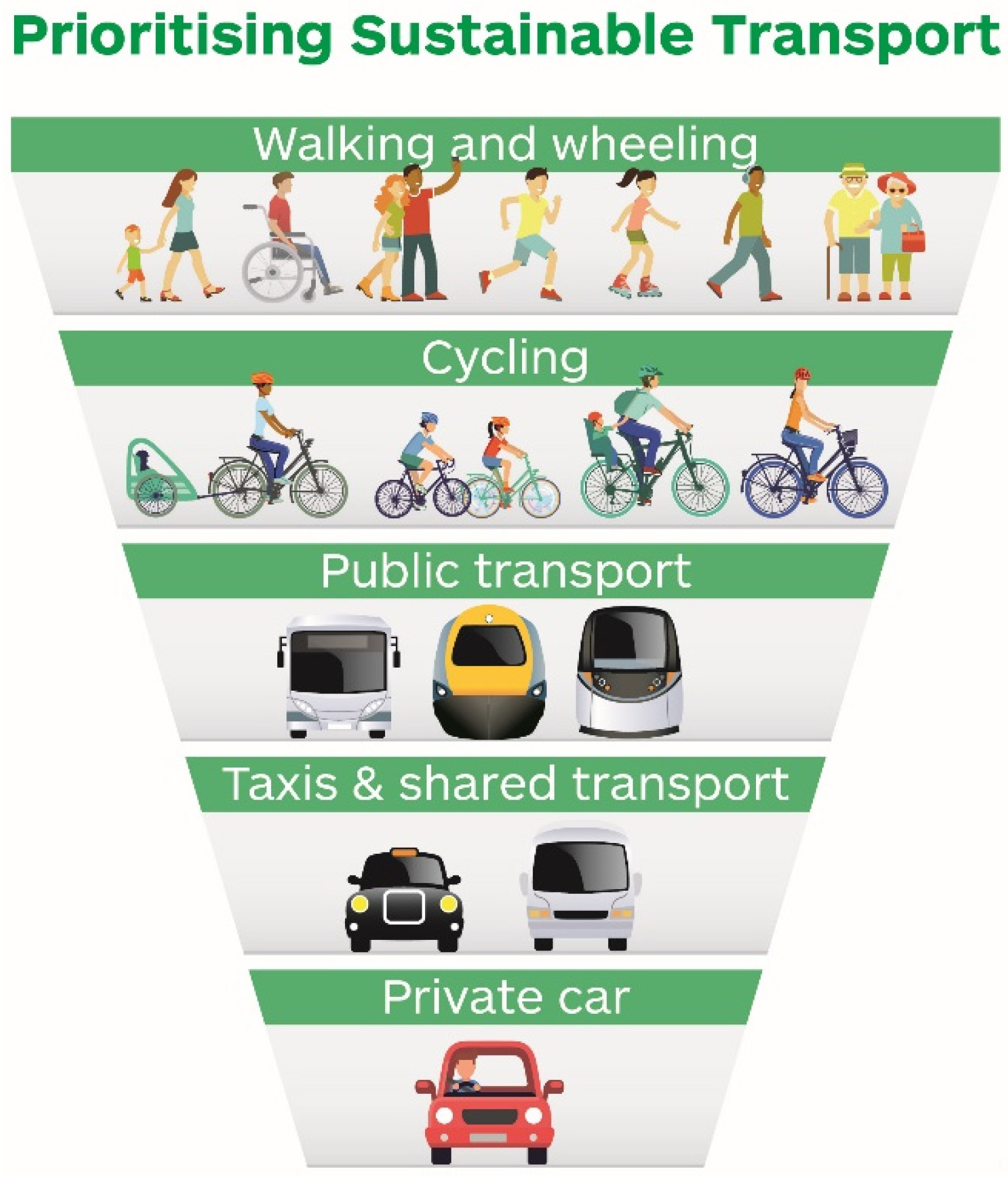
2.3. Sustainable Transport
3. Current State
4. Methodology
5. Results
6. Discussion
7. Conclusions
Author Contributions
Funding
Data Availability Statement
Acknowledgments
Conflicts of Interest
References
- Dvořák, Z.; Sventeková, E.; Řehák, D.; Čekerevac, Z. Assessment of Critical Infrastructure Elements in Transport. Procedia Eng. 2017, 187, 548–555. [Google Scholar] [CrossRef]
- European Council. Council Directive 2008/114/EC of 8 December 2008 on the Identification and Designation of European Critical Infrastructures and the Assessment of the Need to Improve their Protection; European Council: Brussels, Belgium, 2008. [Google Scholar]
- Řehák, D.; Patrman, D.; Brabcová, V.; Dvořák, Z. Identifying Critical Elements of Road Infrastructure Using Cascading Impact Assessment. Transport 2020, 35, 300–314. [Google Scholar] [CrossRef]
- Hoterová, K.; Dvořák, Z. Comparison of CO2 emissions in rail and road transport. Doprava a Životní Prostředí 2020. [Google Scholar]
- Regulation of the European Parliament and of the Council Amending Regulation (EU) 2018/842 on Binding Annual Greenhouse Gas Emission Reductions by Member States from 2021 to 2030 Contributing to Climate Action to Meet Commitments under the Paris Agreement and Amending Regulation. Available online: https://eur-lex.europa.eu/legal-content/EN/TXT/PDF/?uri=CELEX:32018R0842&from=EN (accessed on 15 August 2021).
- Chen, L.-W.A.; Chien, L.-C.; Li, Y.; Lin, G. Nonuniform impacts of COVID-19 lockdown on air quality over the United States. Sci. Total Environ. 2020, 745, 141105. [Google Scholar] [CrossRef]
- Zambrano-Monserrate, M.A.; Ruano, M.A.; Sanchez-Alcalde, L. Indirect effects of COVID-19 on the environment. Sci. Total Environ. 2020, 728, 138813. [Google Scholar] [CrossRef]
- Nie, D.; Shen, F.; Wang, J.; Ma, X.; Li, Z.; Ge, P.; Ou, Y.; Jiang, Y.; Chen, M.; Chen, M.; et al. Changes of air quality and its associated health and economic burden in 31 provincial capital cities in China during COVID-19 pandemic. Atmos. Res. 2020, 249, 105328. [Google Scholar] [CrossRef] [PubMed]
- Shi, X.; Brasseur, G.P. The Response in Air Quality to the Reduction of Chinese Economic Activities during the COVID-19 Outbreak. Geophys. Res. Lett. 2020, 47. [Google Scholar] [CrossRef]
- Li, L.; Li, Q.; Huang, L.; Wang, Q.; Zhu, A.; Xu, J.; Liu, Z.; Li, H.; Shi, L.; Li, R.; et al. Air quality changes during the COVID-19 lockdown over the Yangtze River Delta Region: An insight into the impact of human activity pattern changes on air pollution variation. Sci. Total Environ. 2020, 732, 139282. [Google Scholar] [CrossRef]
- Muhammad, S.; Long, X.; Salman, M. COVID-19 pandemic and environmental pollution: A blessing in disguise? Sci. Total Environ. 2020, 728, 138820. [Google Scholar] [CrossRef]
- Silver, B.; He, X.; Arnold, S.R.; Spracklen, D.V. The impact of COVID-19 control measures on air quality in China. Environ. Res. Lett. 2020, 15, 084021. [Google Scholar] [CrossRef]
- Bešinović, N. Resilience in railway transport systems: A literature review and research agenda. Transp. Rev. 2020, 40, 457–478. [Google Scholar] [CrossRef]
- Ližbetinová, L.; Hitka, M.; Soušek, R.; Caha, Z. Motivational preferences within job positions are different: Empirical study from the Czech transport and logistics enterprises. Econ. Res. Ekonomska Istraživanja 2020, 34, 2387–2407. [Google Scholar] [CrossRef]
- Chu, Z. Logistics and economic growth: A panel data approach. Ann. Reg. Sci. 2011, 49, 87–102. [Google Scholar] [CrossRef]
- Arshed, N.; Hassan, M.S.; Khan, M.U.; Uppal, A.A. Moderating Effects of Logistics Infrastructure Development and Real Sector Productivity: A Case of Pakistan. Glob. Bus. Rev. 2019. [Google Scholar] [CrossRef]
- Vavrek, R.; Bečica, J. Capital City as a Factor of Multi-Criteria Decision Analysis—Application on Transport Companies in the Czech Republic. Mathematics 2020, 8, 1765. [Google Scholar] [CrossRef]
- Patrman, D.; Šplíchalová, A.; Řehák, D.; Onderková, V. Factors Influencing the Performance of Critical Land Transport Infrastructure Elements. Transp. Res. Procedia 2019, 40, 1518–1524. [Google Scholar] [CrossRef]
- Buehler, R. Can Public Transportation Compete with Automated and Connected Cars? J. Public Transp. 2018, 21, 7–18. [Google Scholar] [CrossRef] [Green Version]
- Bruun, E.; Vanderschuren, M. Assessment Methods from Around the World Potentially Useful for Public Transport Projects. J. Public Transp. 2017, 20, 103–130. [Google Scholar] [CrossRef] [Green Version]
- Foltýnová, H.B.; Vejchodská, E.; Rybová, K.; Květoň, V. Sustainable urban mobility: One definition, different stakeholders’ opinions. Transp. Res. Part D Transp. Environ. 2020, 87, 102465. [Google Scholar] [CrossRef]
- Li, R.; Yang, F.; Liu, Z.; Shang, P.; Wang, H. Effect of taxis on emissions and fuel consumption in a city based on license plate recognition data: A case study in Nanning, China. J. Clean. Prod. 2019, 215, 913–925. [Google Scholar] [CrossRef]
- Euchi, J.; Kallel, A. Internalization of external congestion and CO2emissions costs related to road transport: The case of Tunisia. Renew. Sustain. Energy Rev. 2021, 142, 110858. [Google Scholar] [CrossRef]
- Du, J.; Rakha, H.A.; Filali, F.; Eldardiry, H. COVID-19 pandemic impacts on traffic system delay, fuel consumption and emissions. Int. J. Transp. Sci. Technol. 2020, 10, 184–196. [Google Scholar] [CrossRef]
- Babak, N. Transport Construction Negative Impact on the Environment. Procedia Eng. 2017, 189, 867–873. [Google Scholar] [CrossRef]
- European Commission. Special Eurobarometer 468: Attitudes of European Citizens towards the Environment; European Union: Brussels, Belgium, 2021. [Google Scholar]
- Skirienė, A.; Stasiškienė, Ž. COVID-19 and Air Pollution: Measuring Pandemic Impact to Air Quality in Five European Countries. Atmosphere 2021, 12, 290. [Google Scholar] [CrossRef]
- European Environmental Agency. Explaining Road Transport Emissions: A Non-Technical Guide. Available online: https://www.eea.europa.eu/publications/explaining-road-transport-emissions (accessed on 20 May 2021).
- European Union. Monitoring CO2 Emissions from Passenger Cars and Vans in 2018. Available online: https://www.eea.europa.eu/publications/co2-emissions-from-cars-and-vans-2018 (accessed on 15 May 2021).
- Ventura, L.M.B.; Ramos, M.B.; D’Agosto, M.D.A.; Gioda, A. Evaluation of the impact of the national strike of the road freight transport sector on the air quality of the metropolitan region of Rio de Janeiro, Brazil. Sustain. Cities Soc. 2020, 65, 102588. [Google Scholar] [CrossRef]
- Zhai, M.; Wolff, H. Air pollution and urban road transport: Evidence from the world’s largest low-emission zone in London. Environ. Econ. Policy Stud. 2021, 23, 721–748. [Google Scholar] [CrossRef]
- Air Quality in Europe—2013 Report. Available online: https://www.eea.europa.eu/publications/air-quality-in-europe-2013 (accessed on 20 May 2021).
- Climate Change 2013, the Physical Science Basis. Available online: https://www.cambridge.org/core/books/climate-change-2013-the-physical-science-basis/BE9453E500DEF3640B383BADDC332C3E (accessed on 15 May 2021).
- Sagnotti, L.; Taddeucci, J.; Winkler, A.; Cavallo, A. Compositional, morphological, and hysteresis characterization of magnetic airborne particulate matter in Rome, Italy. Geochem. Geophys. Geosyst. 2009, 10. [Google Scholar] [CrossRef]
- Lei, R.; Feng, S.; Lauvaux, T. Country-Scale Trends in Air Pollution and Fossil Fuel CO2 Emissions during 2001–2018: Confronting the Roles of National Policies and Economic Growth. Environ. Res. Lett. 2020, 16, 014006. [Google Scholar] [CrossRef]
- Sui, X.; Qi, K.; Nie, Y.; Ding, N.; Shi, X.; Wu, X.; Zhang, Q.; Wang, W. Air quality and public health risk assessment: A case study in a typical polluted city, North China. Urban Clim. 2021, 36, 100796. [Google Scholar] [CrossRef]
- Vassilara, F.; Spyridaki, A.; Pothitos, G.; Deliveliotou, A.; Papadopoulos, A. A Rare Case of Human Coronavirus 229E Associated with Acute Respiratory Distress Syndrome in a Healthy Adult. Case Rep. Infect. Dis. 2018, 2018, 6796839. [Google Scholar] [CrossRef] [PubMed] [Green Version]
- AminJafari, A.; Ghasemi, S. The possible of immunotherapy for COVID-19: A systematic review. Int. Immunopharmacol. 2020, 83, 106455. [Google Scholar] [CrossRef]
- Jansen, J.H.; Day, R.L. A novel presentation of COVID-19 via community acquired infection. Vis. J. Emerg. Med. 2020, 20, 100760. [Google Scholar] [CrossRef]
- Contentti, E.C.; Correa, J. Immunosuppression during the COVID-19 pandemic in neuromyelitis optica spectrum disorders patients: A new challenge. Mult. Scler. Relat. Disord. 2020, 41, 102097. [Google Scholar] [CrossRef]
- Boccaletti, S.; Ditto, W.; Mindlin, G.; Atangana, A. Modeling and forecasting of epidemic spreading: The case of COVID-19 and beyond. Chaos, Solitons Fractals 2020, 135, 109794. [Google Scholar] [CrossRef]
- González-Sánchez, G.; Olmo-Sánchez, M.; Maeso-González, E. Challenges and Strategies for Post-COVID-19 Gender Equity and Sustainable Mobility. Sustainability 2021, 13, 2510. [Google Scholar] [CrossRef]
- Zhang, J.; Hayashi, Y.; Frank, L.D. COVID-19 and transport: Findings from a world-wide expert survey. Transp. Policy 2021, 103, 68–85. [Google Scholar] [CrossRef]
- Anke, J.; Francke, A.; Schaefer, L.-M.; Petzoldt, T. Impact of SARS-CoV-2 on the mobility behaviour in Germany. Eur. Transp. Res. Rev. 2021, 13, 1–13. [Google Scholar] [CrossRef]
- Cui, Q.; He, L.; Liu, Y.; Zheng, Y.; Wei, W.; Yang, B.; Zhou, M. The impacts of COVID-19 pandemic on China’s transport sectors based on the CGE model coupled with a decomposition analysis approach. Transp. Policy 2021, 103, 103–115. [Google Scholar] [CrossRef]
- Khomsi, K.; Najmi, H.; Amghar, H.; Chelhaoui, Y.; Souhaili, Z. COVID-19 national lockdown in morocco: Impacts on air quality and public health. One Health 2020, 11, 100200. [Google Scholar] [CrossRef]
- Pardo, C.F.; Zapata-Bedoya, S.; Ramirez-Varela, A.; Ramirez-Corrales, D.; Espinosa-Oviedo, J.-J.; Hidalgo, D.; Rojas, N.; González-Uribe, C.; García, J.D.; Cucunubá, Z.M. COVID-19 and public transport: An overview and recommendations applicable to Latin America. Infectio 2021, 25, 182. [Google Scholar] [CrossRef]
- Hiselius, L.W.; Arnfalk, P. When the impossible becomes possible: COVID-19’s impact on work and travel patterns in Swedish public agencies. Eur. Transp. Res. Rev. 2021, 13, 1–10. [Google Scholar] [CrossRef]
- Vickerman, R. Will Covid-19 put the public back in public transport? A UK perspective. Transp. Policy 2021, 103, 95–102. [Google Scholar] [CrossRef]
- Aloi, A.; Alonso, B.; Benavente, J.; Cordera, R.; Echániz, E.; González, F.; Ladisa, C.; Lezama-Romanelli, R.; López-Parra, R.; Mazzei, V.; et al. Effects of the COVID-19 Lockdown on Urban Mobility: Empirical Evidence from the City of Santander (Spain). Sustainability 2020, 12, 3870. [Google Scholar] [CrossRef]
- Jenelius, E.; Cebecauer, M. Impacts of COVID-19 on public transport ridership in Sweden: Analysis of ticket validations, sales and passenger counts. Transp. Res. Interdiscip. Perspect. 2020, 8, 100242. [Google Scholar] [CrossRef] [PubMed]
- Siciliano, B.; Carvalho, G.; da Silva, C.M.; Arbilla, G. The Impact of COVID-19 Partial Lockdown on Primary Pollutant Concentrations in the Atmosphere of Rio de Janeiro and São Paulo Megacities (Brazil). Bull. Environ. Contam. Toxicol. 2020, 105, 2–8. [Google Scholar] [CrossRef]
- Sharma, S.; Zhang, M.; Anshika; Gao, J.; Zhang, H.; Kota, S.H. Effect of restricted emissions during COVID-19 on air quality in India. Sci. Total Environ. 2020, 728, 138878. [Google Scholar] [CrossRef] [PubMed]
- Bar, S.; Parida, B.R.; Mandal, S.P.; Pandey, A.C.; Kumar, N.; Mishra, B. Impacts of partial to complete COVID-19 lockdown on NO2 and PM2.5 levels in major urban cities of Europe and USA. Cities 2021, 117, 103308. [Google Scholar] [CrossRef] [PubMed]
- Beloconi, A.; Probst-Hensch, N.M.; Vounatsou, P. Spatio-temporal modelling of changes in air pollution exposure asso-ciated to the COVID-19 lockdown measures across Europe. Sci. Total Environ. 2021, 787, 1–11. [Google Scholar] [CrossRef]
- Filonchyk, M.; Hurynovich, V.; Yan, H. Impact of COVID-19 Pandemic on Air Pollution in Poland Based on Surface Measurements and Satellite Data. Aerosol Air Qual. Res. 2021, 21, 200472. [Google Scholar] [CrossRef]
- Bitta, J.; Svozilík, V.; Krakovská, A.S. Effect of the COVID-19 Lockdown on Air Pollution in the Ostrava Region. Int. J. Environ. Res. Public Health 2021, 18, 8265. [Google Scholar] [CrossRef]
- Matthias, V.; Quante, M.; Arndt, J.A.; Badeke, R.; Fink, L.; Petrik, R.; Feldner, J.; Schwarzkopf, D.; Link, E.-M.; Ramacher, M.O.P.; et al. The role of emission reductions and the meteorological situation for air quality improvements during the COVID-19 lockdown period in central Europe. Atmos. Chem. Phys. Discuss. 2021, 21, 13931–13971. [Google Scholar] [CrossRef]
- Solberg, S.; Walker, S.-E.; Schneider, P.; Guerreiro, C. Quantifying the Impact of the Covid-19 Lockdown Measures on Nitrogen Dioxide Levels throughout Europe. Atmosphere 2021, 12, 131. [Google Scholar] [CrossRef]
- Veselík, P.; Sejkorová, M.; Nieoczym, A.; Caban, J. Outlier Identification of Concentrations of Pollutants in Environmental Data Using Modern Statistical Methods. Pol. J. Environ. Stud. 2019, 29, 853–860. [Google Scholar] [CrossRef]
- Kimbrell, C.M. Electric carsharing and the sustainable mobility transition: Conflict and contestation in a Czech actor-network. Energy Res. Soc. Sci. 2021, 74, 101971. [Google Scholar] [CrossRef]
- Acheampong, R.A.; Cugurullo, F.; Gueriau, M.; Dusparic, I. Can autonomous vehicles enable sustainable mobility in future cities? Insights and policy challenges from user preferences over different urban transport options. Cities 2021, 112, 103134. [Google Scholar] [CrossRef]
- Pamucar, D.; Deveci, M.; Canıtez, F.; Paksoy, T.; Lukovac, V. A Novel Methodology for Prioritizing Zero-Carbon Measures for Sustainable Transport. Sustain. Prod. Consum. 2021, 27, 1093–1112. [Google Scholar] [CrossRef]
- Faulin, J.; Grasman, S.; Juan, A.; Hirsch, P. Sustainable Transportation and Smart Logistics: Decision-Making Models and Solutions; Elsevier: Amsterdam, The Netherlands, 2019; p. 534. [Google Scholar]
- Sustainable Travel and the National Transport Strategy. Available online: https://www.transport.gov.scot/active-travel/developing-an-active-nation/sustainable-travel-and-the-national-transport-strategy/# (accessed on 25 August 2021).
- Ku, D.; Bencekri, M.; Kim, J.; Leec, S.; Leed, S. Review of European Low Emission Zone Policy. Chem. Eng. 2020, 78, 241–246. [Google Scholar] [CrossRef]
- Pettersson, F.; Stjernborg, V.; Curtis, C. Critical challenges in implementing sustainable transport policy in Stockholm and Gothenburg. Cities 2021, 113, 103153. [Google Scholar] [CrossRef]
- Kua, D.; Kwaka, J.; Naa, S.; Leeb, S.; Leea, S. Impact Assessment on Cycle Super Highway Schemes. Chem. Eng. 2021, 83, 181–186. [Google Scholar] [CrossRef]
- Desta, R.; Tóth, J. Simulating the performance of integrated bus priority setups with microscopic traffic mockup experiments. Sci. Afr. 2021, 11, e00707. [Google Scholar] [CrossRef]
- Abduljabbar, R.L.; Liyanage, S.; Dia, H. The role of micro-mobility in shaping sustainable cities: A systematic literature review. Transp. Res. Part D Transp. Environ. 2021, 92, 102734. [Google Scholar] [CrossRef]
- González, L.; Cordero-Moreno, D.; Espinoza, J. Public transportation with electric traction: Experiences and challenges in an Andean city. Renew. Sustain. Energy Rev. 2021, 141, 110768. [Google Scholar] [CrossRef]
- National Traffic Census. Available online: http://scitani2016.rsd.cz/pages/map/default.aspx (accessed on 18 October 2021).
- Information on Air Quality in the Czech Republic. Available online: https://www.chmi.cz/files/portal/docs/uoco/web_generator/locality/pollution_locality/loc_ZUHR_CZ.html (accessed on 25 August 2021).
- Keder, J. Evaluation of the State of all Methods of Air Quality Monitoring in Prague; CHMI: Prague, Czech Republic, 2001. [Google Scholar]
- User Manual Models T200 and T200U. Available online: http://www.teledyne-api.com/prod/Downloads/T200%20%26%20T200U%20NVS%20Manual%20-%20083730200.pdf (accessed on 15 May 2021).
- Technical Manual MP101M. Available online: http://norditech.com.au/wp-content/uploads/2019/09/MP101M_User_Manual_Eng_14.04.pdf (accessed on 15 May 2021).
- Information on Air Quality in the Czech Republic. Available online: https://www.chmi.cz/files/portal/docs/uoco/historicka_data/OpenIsko_data/index.html (accessed on 25 August 2021).
- Johnson, R.A.; Wichern, D.W. Applied Multivariate Statistical Analysis; Prentice-Hall International: Englewood Cliffs, UK, 1992; p. 642. [Google Scholar]
- Andel, J. Basics of Mathematical Statistics, 2nd ed.; MATFYZPRES: Prague, Czech Republic, 2007; p. 360. [Google Scholar]


| Traffic Counting | Timing | Intensity |
|---|---|---|
| Annual average of daily traffic intensity—all days | vehicle/day | 23,413 |
| Annual average of daily traffic intensity—workdays | vehicle/day | 25,413 |
| Annual average of daily traffic intensity—free days | vehicle/day | 18,412 |
| Fifty times traffic intensity | vehicle/hour | 2477 |
| Peak-hour traffic intensity | vehicle/hour | 2295 |
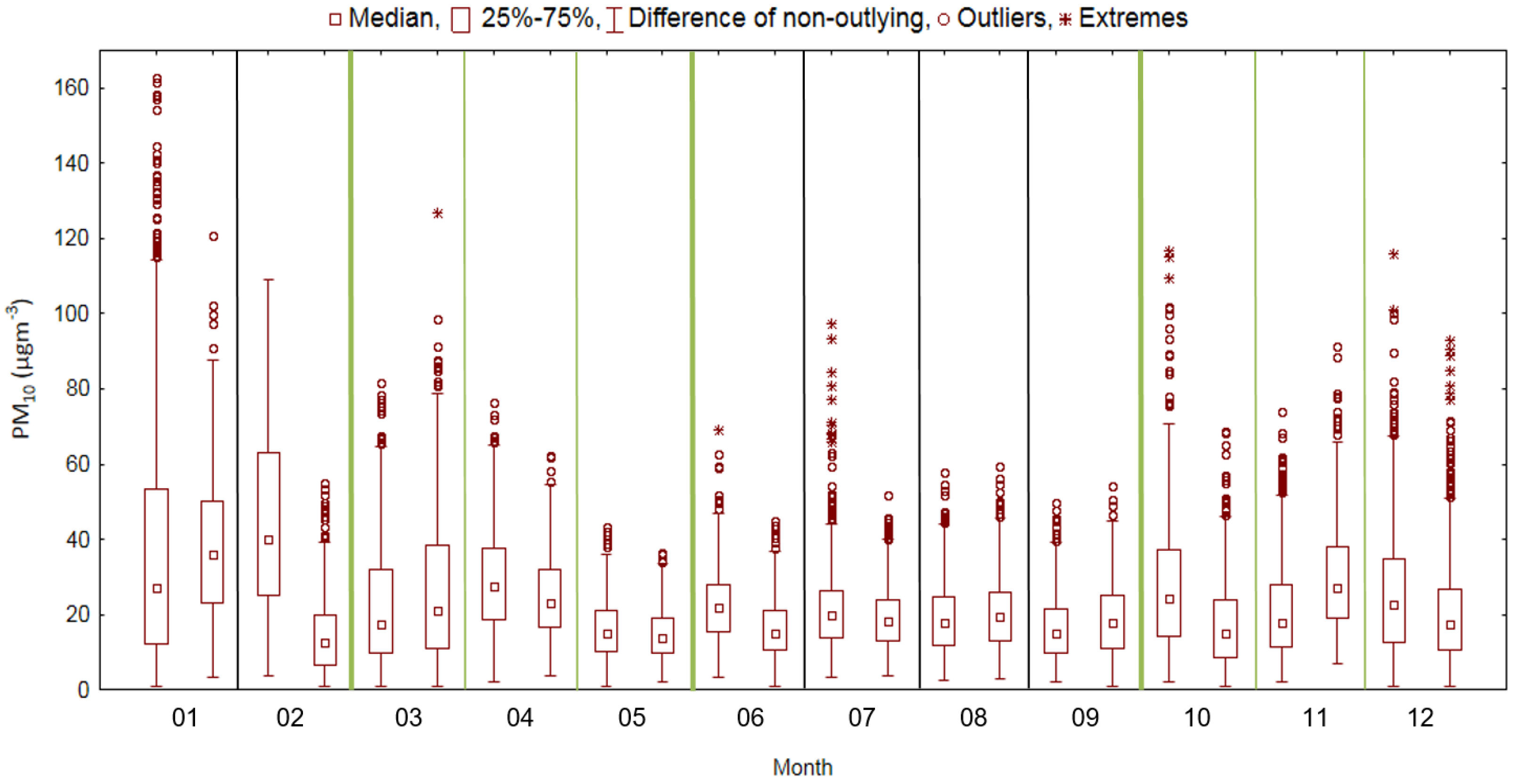
| PM10 | Mean | Median | Min | Max | SD | |||||
|---|---|---|---|---|---|---|---|---|---|---|
| Month | 2019 | 2020 | 2019 | 2020 | 2019 | 2020 | 2019 | 2020 | 2019 | 2020 |
| January | 34.74 | 37.82 | 27.20 | 36.05 | 1.00 | 3.20 | 162.90 | 102.82 | 35.06 | 20.36 |
| February | 44.80 | 14.81 | 40.00 | 12.60 | 3.80 | 1.00 | 109.00 | 55.10 | 24.62 | 10.35 |
| March | 22.50 | 26.93 | 17.20 | 20.90 | 1.00 | 1.00 | 81.60 | 126.90 | 17.06 | 20.38 |
| April | 28.60 | 24.96 | 27.60 | 23.05 | 2.00 | 3.60 | 76.40 | 62.30 | 13.60 | 10.92 |
| May | 16.12 | 14.70 | 14.90 | 16.65 | 1.00 | 2.10 | 43.40 | 36.20 | 8.12 | 6.98 |
| June | 22.36 | 16.33 | 21.80 | 15.00 | 3.40 | 1.00 | 69.00 | 44.70 | 9.53 | 8.07 |
| July | 21.57 | 17.78 | 19.70 | 18.10 | 3.40 | 3.80 | 97.20 | 51.90 | 12.04 | 7.90 |
| August | 19.07 | 20.56 | 17.70 | 19.30 | 2.40 | 2.70 | 57.90 | 59.20 | 9.64 | 10.07 |
| September | 16.31 | 18.24 | 14.90 | 17.70 | 2.20 | 1.00 | 49.80 | 54.30 | 8.43 | 9.61 |
| October | 27.87 | 17.45 | 24.25 | 14.80 | 2.00 | 1.00 | 116.60 | 68.60 | 18.35 | 11.40 |
| November | 21.25 | 29.40 | 17.80 | 27.20 | 2.10 | 7.00 | 73.90 | 91.40 | 12.92 | 14.00 |
| December | 25.98 | 21.24 | 22.80 | 17.40 | 1.00 | 1.00 | 115.80 | 92.90 | 17.49 | 15.22 |
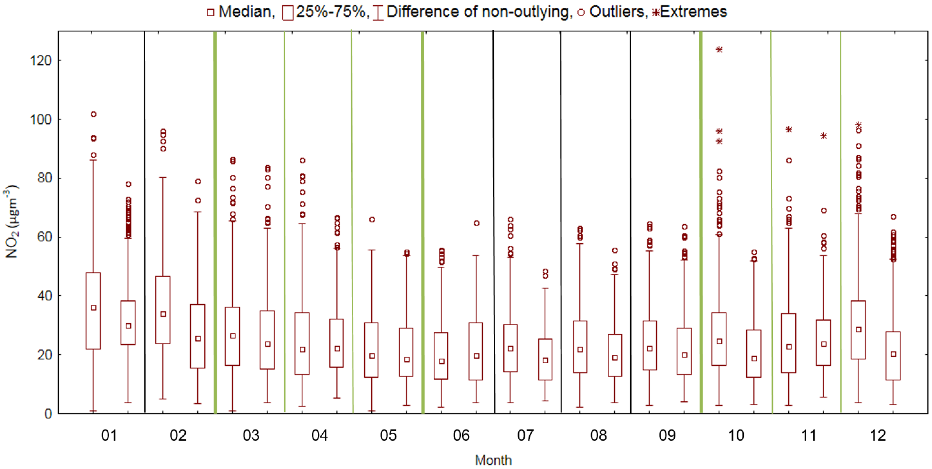
| NO2 | Mean | Median | Min | Max | SD | |||||
|---|---|---|---|---|---|---|---|---|---|---|
| Month | 2019 | 2020 | 2019 | 2020 | 2019 | 2020 | 2019 | 2020 | 2019 | 2020 |
| January | 35.94 | 31.62 | 36.20 | 30.00 | 1.00 | 3.80 | 101.80 | 78.00 | 17.73 | 12.38 |
| February | 35.98 | 27.44 | 34.00 | 25.60 | 5.00 | 3.30 | 96.20 | 79.00 | 16.72 | 14.28 |
| March | 27.33 | 26.06 | 26.60 | 23.70 | 1.00 | 3.80 | 86.50 | 83.60 | 14.75 | 14.02 |
| April | 25.18 | 25.01 | 22.00 | 22.20 | 2.50 | 5.40 | 86.10 | 66.60 | 15.17 | 12.00 |
| May | 22.22 | 21.35 | 19.90 | 18.60 | 1.00 | 2.90 | 66.00 | 55.10 | 12.02 | 10.94 |
| June | 20.79 | 21.64 | 18.00 | 19.70 | 2.10 | 3.80 | 55.50 | 64.80 | 11.37 | 11.65 |
| July | 23.43 | 19.06 | 22.30 | 18.30 | 3.60 | 4.40 | 66.00 | 48.60 | 10.99 | 8.83 |
| August | 23.11 | 20.64 | 21.80 | 19.30 | 2.30 | 3.60 | 63.10 | 55.50 | 11.65 | 9.90 |
| September | 24.35 | 22.03 | 22.20 | 20.10 | 2.90 | 4.00 | 64.70 | 63.70 | 11.70 | 11.24 |
| October | 26.68 | 20.82 | 24.70 | 18.90 | 2.90 | 3.10 | 123.80 | 54.90 | 14.56 | 10.63 |
| November | 25.24 | 24.72 | 22.80 | 23.70 | 2.70 | 5.50 | 96.60 | 94.50 | 14.55 | 10.49 |
| December | 30.09 | 21.74 | 27.70 | 20.30 | 3.60 | 3.10 | 98.10 | 67.00 | 15.88 | 12.61 |
| AHF | F | p-Value | AHt | t | p-Value | |
|---|---|---|---|---|---|---|
| PM10 | σ12 ≠ σ22 | 1.072 * | 0.005 * | µ1> µ2 | 4.228 * | 0.000 * |
| NO2 | σ12 ≠ σ22 | 1.074 * | 0.005 * | µ1> µ2 | 5.414 * | 0.000 * |
Publisher’s Note: MDPI stays neutral with regard to jurisdictional claims in published maps and institutional affiliations. |
© 2021 by the authors. Licensee MDPI, Basel, Switzerland. This article is an open access article distributed under the terms and conditions of the Creative Commons Attribution (CC BY) license (https://creativecommons.org/licenses/by/4.0/).
Share and Cite
Vichova, K.; Veselik, P.; Heinzova, R.; Dvoracek, R. Road Transport and Its Impact on Air Pollution during the COVID-19 Pandemic. Sustainability 2021, 13, 11803. https://doi.org/10.3390/su132111803
Vichova K, Veselik P, Heinzova R, Dvoracek R. Road Transport and Its Impact on Air Pollution during the COVID-19 Pandemic. Sustainability. 2021; 13(21):11803. https://doi.org/10.3390/su132111803
Chicago/Turabian StyleVichova, Katerina, Petr Veselik, Romana Heinzova, and Radek Dvoracek. 2021. "Road Transport and Its Impact on Air Pollution during the COVID-19 Pandemic" Sustainability 13, no. 21: 11803. https://doi.org/10.3390/su132111803