Establishing a Sustainable Labor Market in Developing Countries: A Perspective of Generational Differences in Household Wage

Abstract

The importance of a sustainable labor market is a critical and fundamental point for many developing countries, where global competitiveness is based on cheap labor. The aim of this empirical–analytical study, framed in China in the research context, is to approach this hot topic from the lens of household wage differences between generations. Using cross-sectional data, consisting of the China Dynamic Migrant Survey and Oaxaca-Blinder decomposition methods and quantiles, to analyze the data results confirmed the differences in wages between two generations of peasant and urban workers. Moreover, a distinctive tapering in the pay gap occurred among the new generation. Fundamentally, a big gap exists in the rate of return on education between urban and rural labor. According to the results of quantile decomposition, the old generation of peasant and urban workers demonstrate anti-discriminatory phenomena at very low and very high scores.

1. Introduction

With the continuous promotion of marketization, industrialization, and urbanization, a high number of surplus rural labor force keeps flowing into cities and towns for employment, thus forming the group of “migrant workers” with Chinese characteristics. The return rate of education investment of migrant workers in the urban labor market is significantly lower than that of urban workers, after controlling for gender, age, health level, industry, and other factors [1,2]. Therefore, the Chinese government has been committed to expanding employment opportunities for the rural labor force and encouraging employment among migrant workers through various channels. However, considering China’s long-term planned economy era, an obvious difference exists in the census register between urban and rural labor wages, with significant benefits according to era characteristics.

Extensive, and in-depth analysis has been carried out on the two generations of migrant workers in China to date. The research focuses on two aspects. One of these aspects is the differences in individual characteristics between the new and old generations of migrant workers [3,4,5]; these studies compare the differences in individual characteristics, such as human capital, employment stability rate, the gender ratio, and the health status of new and old farmers and migrant workers. The second area of research refers to the subjective cognitive differences between two generations [6]. The new generation of migrant workers have high career expectations and are highly willing to integrate into urban life, owing to the obvious differences in culture, concept, and behavior. Although the existing research results contain relevant literature on the inter-generational differences among migrant workers, they rarely analyze the inter-generational differences in wage discrimination between migrant and urban workers. The academic circles have carried out deep research on the relationship between household registration discrimination and urban–rural wage differences from the literature review. However, few scholars have conducted comparative studies on household registration discrimination in the gender-specific labor market. Therefore, based on the existing research gap, this study selected the latest data and used two regression methods and two wage difference decomposition methods to estimate and decompose the gender-specific urban and rural labor wage difference, aiming to analyze the gender differences in urban and rural household registration discrimination. This study is expected to enrich the understanding of the wage differences between different labor groups and provide particular reference suggestions for the government to formulate relevant policies.

2. Literature Review

In 2011, “A Report on the Comprehensive Policy Recommendations for the Program of Young Migrant Workers in China”, released by the Chinese Academy of Social Sciences, showed that the wage level of urban workers was more than three times that of young migrant workers. Although the government has issued a series of policies to break down the geographical barriers between urban and rural areas, the country has not fundamentally reformed the household registration system. Given this lack of reform, the phenomenon of “different pay for the same work” in urban and rural labor force has become widespread; that is, the problem of household registration discriminating against migrant workers has never been completely solved in the labor market. Markets can be divided into several distinct sub-markets, each of which has a different employment opportunity allocation mechanism and wage determination mechanism. The income gap between migrant workers and urban workers in 2002 was almost entirely due to factor endowment, especially the gap in education level [7,8]. In China’s urban labor market, an insurmountable gap exists between the wages of urban registered workers and those of migrant workers, which has been accepted by most people. Even after controlling for human capital (education, work experience, training), enterprise characteristics (enterprise ownership type, etc.), individual characteristics (gender, marital status), and other factors that may affect wage level, significant wage differences remained between urban workers and farmers [9,10,11].This issue has been extensively discussed in the domestic literature, and research results show that household registration discrimination is the main cause of the wage differences between urban and rural labor [3,12]. Several scholars have analyzed the wage differences between urban and rural labor forces from the perspective of wage distribution [13,14,15]. Other studies have shown that household registration discrimination is not the main cause of wage differences; instead, personal characteristics are considered the key factor [16,17]. However, most studies ignore the inter-generational differences in wage differences between urban and rural labor forces caused by household registration discrimination. With the continuous opening of the market and the continuous relaxation of household registration restrictions, the wage difference between new and old generations of migrant and urban workers will inevitably change.

In China, discrimination exists between rural and urban migrants due to the peculiar hukou system, which is the household registration system. This system is a national policy, in which an individual’s inheritable status, based on his/her residence, continuously represents one’s social and economic status, ultimately leading to the household registration and intergroup discrimination [18]. Most scholars have proposed that household registration discrimination is the root cause of the differential treatment between urban workers and peasant workers, which is most reflected in the varying wages for the same kind of work [19]. Other scholars considered that the differences in the individual characteristics of urban and country workers are the main reason for the difference in the wages [14]. Moreover, household discrimination leads to an asymmetric distribution of wages, demonstrating differential treatment when choosing employment opportunities [20,21]. The Chinese economy has many features that the Lewis model attempts to capture. Islam and Yokota (2006) examine national-level wages in China and province level manufacturing wages for Beijing, Shanghai, Guizhou and Gansu [22]. Bu et al. found a significant wage gap between migrant workers and urban labor, but the intergenerational gap tends to decrease, which is a good phenomenon [23]. Labor marker segregation or wage differences are common phenomena in developing countries [24]. In Vietnam, owing to the new economic opportunities and market reform, rural residents were attracted to migrate to urban areas. Vietnam has a similar household registration system to China, called ho khau, which also impedes pay equity. It has been suggested that provincial officials encouraging employers to give priority to urban residents or to require skilled and well-educated workers, potentially aggravating the wage differences between urban and rural residents [25].

Based on the household registration (hukou) system, China has been divided into urban and rural population groups in terms of society, economics and politics. Rural migrants refer to second-class citizens, who are ineligible for settlement in cities and other welfare and services because of their rural hukou [26]. Agglomeration and congestion effects lead to high- and low-order cities. Additionally, migrants with urban hukou move into these higher order cities, which is called urban migrantion [27]. Migrant workers born in between the 1980s and 1990s accounted for 50.5% of the total number of migrant workers in China as of 2017; they are called the new generation of migrant workers [19,22]. Unlike previous generations, they require higher-quality jobs, as well as higher wages, with the shortest possible working hours and a better quality of urban life [25]. They no longer only seek to meet their food and clothing needs, but pursue mental fulfilment, that is, a self-identity, as workers not peasants, and dream of achievement [28]. They are equipped with a higher education, empowering them to defend their legal rights and interests with an aspiring spirit [23]. However, they do not have farming experience and change jobs at a frequent rate, demonstrating their higher priorities of an appealing career, social identity, expectations for life, and urbanization desires compared to the older generation [27]. Compared with older generations, the new generation of migrant workers shows unique characteristics. With the constant flow of the new generation of peasant workers from rural to urban areas, the wage gap between rural and urban areas becomes narrower, although the wage of the new generation is lower than it was the past. Most importantly, household registration discrimination explained the wage difference between urban and rural workers from the old to the new generation, which benefits the urbanization process of migrant workers [28].

The wage assimilation of migrant workers in China was analyzed, and it was found that the wage gap between migrant workers and local urban workers will gradually narrow [29]. The structural effects caused by market discrimination are gradually increasing. Many scholars have divided migrant workers into the old generation and the new generation to analyze the generational differences in household wage. The old generation of migrant workers experienced much more direct household registration discrimination than the new generation, and the discrimination widened the wage gap between rural and urban labor forces [30,31,32,33]. The differences in individual characteristics and the degree of household registration discrimination between migrant workers and urban workers in the new generation have been significantly reduced, and these changes will also reduce the difference in household registration wages [29]. Scholars hold different views regarding the household registration discrimination trends between the two generations of migrant workers. The results of an empirical analysis showed that the new generation of migrant workers suffers more from household registration discrimination than the old generation. Moreover, the difference in the degree of different pay for equal work is the main reason for the intergenerational differences in household registration discrimination.

3. Empirical Research Design

Data Source and Processing

This paper selected the cross-sectional data of a China Migrants Dynamic Survey. The survey is a recent Chinese national, comprehensive, and continuous academic survey project, and it an important data source for the study of Chinese economic and social issues. In the stage of data-processing, we adopt the following principles: (1) according to Chinese labor law and regulations on working age, this paper selected men aged between 16 and 60 and women aged between 16 to 55; given that migrant workers are the research object, non-agricultural work was only selected on the basis of the age limit of this study; (2) this paper excluded individual entrepreneurs and employers owing to the complex income structure of this part of the population; (3) given that this paper focuses on income differences between urban and migrant workers, this paper only selected employees as the sample and excluded samples from agriculture, forestry, animal husbandry, and fishery industries; (4) with 1980 as the cut-off point, those born before 1980 were considered the old generation of migrant workers, and those born after 1980 were considered the new generation. At present, “old generation migrant workers” and “new generation migrant workers” have no conceptual definition. Some scholars believe that the new generation of migrant workers is under 40 years old, based on their year of birth. Some scholars believe that as long as one parent is a migrant worker, their children will be regarded as the new generation of migrant workers. Other scholars consider the differences between the new generation of migrant workers and the old generation of migrant workers in terms of their characteristics. Nonetheless, current labor economics generally regards a birth year of 1980 as the boundary. Those born before 1980 are the old generation of migrant workers, and those born after 1980 (including those born in 1980) are the new generation of migrant workers [34,35]. This paper obtained a total of 14,694 samples of urban workers, 20,997 samples of the old generation of migrant workers, and 40,722 samples of the new generation of migrant workers, covering 31 provinces (cities and autonomous regions) nationwide.

4. Variable Setting and Descriptive Statistics

4.1. Explanatory Variables

Years of education (educ): According to theory of human capital, the level of human capital is the key factor determining the income level of workers, and a significant positive relationship exists between the two. As the first element of human capital, education plays an important role in workers’ income. Moreover, this paper adopts different educational levels, with the actual number of years of education, rather than the traditional ones used to facilitate the calculation of educational returns. The unit used is years, and the other variables are as follows:

• Work experience (exper.): Given that obtaining accurate data on workers’ work experience is difficult, the paper is based on the work of [9,36]: the actual age of the individual, minus the number of years of education, minus six, is used as a substitute variable for the worker’s work experience. According to Chinese labor laws, if the education level is below junior middle school, people must be at least 16 years old to work; accordingly, their work experience is expressed as age minus 16.
• Marital status (marriage): This paper considers the effects of having a spouse on the income level of workers; thus, the samples marked as cohabitation are classified as those with a spouse. Therefore, marital status is divided into those who are married and those who are not. The former is assigned a value of 1, and the latter is assigned a value of 0.
• Gender (gender): Given that gender wage differences are evident in the Chinese labor market, gender was deliberately considered in the regression, with male respondents assigned a value of 1 and female respondents assigned a value of 0. Owing to the generational differences studied in this paper, gender variables were included in the mixed sample regression model.
• Occupation type (proff): Different occupations may affect the labor income of urban and rural employees in two ways. First, different professions have different requirements regarding the human capital of employees, resulting differences in labor factor returns among occupations. Second, the fragmentation of the labor market leads to barriers to workers’ mobility in different occupations, resulting in income differentials.
• Industry variable (year): Different industries will affect the labor income of employees; thus, different industries are divided into control variables. A total of 20 industries are divided in this paper according to the national industry standard. The classification of occupations and industries used in this paper is based on Chinese standards. As this paper studies the problem of migrant workers in China, it is appropriate to use Chinese standards for related occupations and industries.
• Characteristic variable of unit ownership: The ownership characteristics of the employment sector will affect the labor income of employees; thus, different ownership characteristics are divided as control variables.
• Region variable (region): A big gap exists in the economic development levels in different regions of China. Therefore, the income gap between different regions is significant. The regional dummy variable was introduced to control this influence. If all the 31 provincial administrative regions in Mainland China are included in the model as dummy variables, then a large degree of freedom will be lost. In fact, in previous studies, the majority of scholars divided China into 3–4 regions to control this influence. Generally speaking, China is divided into eastern, central, western, and northeastern regions according to economic development.

4.2. Descriptive Statistics

This paper takes the natural logarithm of hourly wage income as the explained variable, and the explanatory variables include personal characteristics, job characteristics, and regional variables. The averages of urban workers, the old generation of migrant workers, and the new generation of migrant workers are assigned to each variable. This paper also focuses on the differences between educational level and work experience, two major explanatory variables, among the three groups; then, it shows their respective proportions in the population (

Table 1. Descriptive statistics.

	Urban Employees		Old Generation of Migrant Workers		New Generation of Migrant Workers
	V.	S.D.	V.	S.D.	V.	S.D.
Average hourly wage	29.59	33.80	18.66	24.53	19.84	25.68
Average years of education (years)	13.65	2.89	8.64	2.62	11.06	2.76
Average working experience (years)	13.35	9.55	28.65	6.37	9.52	5.58
Degree of education	Amount	%	Amount	%	Amount	%
Graduate	540	3.66	7	0.03	104	0.25
Undergraduate	4272	28.95	148	0.70	2632	6.44
College	3956	26.81	514	2.44	5911	14.47
High school and technical Secondary school	3499	23.71	3012	14.30	11,815	28.93
Junior middle school	2233	15.13	11,630	55.22	18,488	45.27
Primary school or below	256	1.73	5752	27.31	1889	4.63
Group by experience	Amount	%	Amount	%	Amount	%
0 to 10 years	7131	48.33	0	0.00	23,583	57.75
11 to 20 years	4350	29.48	1431	6.79	16,694	40.88
21 to 30 years	2258	15.30	1,2018	57.06	562	1.38
31 years and above	1017	6.89	7614	36.15	0	0.00
Sample size	14,694		20,997		40,772

Notes: V. = Value, S.D. = Standard Deviation.

). The hourly wage of urban workers is higher than that of the other two groups of migrant workers. With respect to the number of years of education, the old generation of migrant workers have the lowest level of education, with most completing their education after only junior high school. Urban workers have the highest level, with most having a high school degree or above, and the average number of years of education is 13.65. In terms of working experience, the average level of working experience for the old generation of migrant workers is higher than that of the other two groups, owing to their older age. The descriptive statistics show the average of various variables for the three different labor force groups. The “standard deviation” in Table 1 is not the standard deviation of the mean, but the standard deviation of the relevant variable. This is the average hourly wage, which is obtained by dividing the sample monthly wage data by the number of hours worked per week and dividing by four.

5. Model Setting and Research Methods

5.1. Salary Regression Equation Setting

The income decision model has long been the focus of labor economics. The human capital income function is obtained by studying the relationship between school education, work experience, and wage income, thus establishing the basic research model of wage equations [9]. The initial form of this model is as follows:

$$\ln {\mathrm{wage}}_{\mathrm{i}}={\beta }_0+{\beta }_{1}educ+{\beta }_2\exp er+{\beta }_3\exp e{r}^2+\epsilon$$

(1)

This is the income determination model, which is an extended form of Mincer’s wage determination model. In this paper, the standard error of robust estimation is chosen. In general, people with higher abilities may have higher education and a higher income, thus omitting the “ability” variable, which overestimates the effect of education on wages, and thus may underestimate the wage difference between urban workers and migrant workers. Further research by Meng et al. found that the impact of education discrimination in the former labor market on the wage gap between urban and rural areas showed a weakening trend in the time dimension [20].

$\log \left(\mathrm{wage}\right)$ is the logarithm of individual;

I’s salary income;

$educ$ denotes the years of education;

$\exp er$ refers to the years of working after finishing school;

$\exp e{r}^2$ is the square of working years, reflecting the relationship between work experience and income;

$\epsilon$ is the random disturbance term, and

$\beta$ is the parameter to be estimated.

The income determination function of Mincer successfully combines theoretical deduction and empirical induction. This function’s theoretical basis is the choice model of education and the absolute model of post-academic training. According to the theory of human capital, laborers acquire the corresponding stock of human capital through human capital investment, such as education and training. After entering the labor market, they obtain an individual labor income through a combination of other production factors. In competitive and non-competitive labor markets, human capital stock has an important effect on the workers’ personal gains. Obtaining a high educational level or training and other activities is an important way for workers to improve their personal income level. Human capital affects and determines labor productivity. Generally, a higher stock of human capital of laborers increases their labor productivity. Therefore, the level of human capital stock determines the income level of workers, and the market mechanism effectively allocates the labor force.

The income-determining equation of Mincer is the cornerstone of empirical analyses of labor income determinants in labor economics. However, the factors influencing workers’ income level are complex. The Mincer income determination equation only considers the influence of the human capital level (reflected by educational level and work experience) on workers’ salary, thereby ignoring the influence of family characteristics, occupation, gender, region, and other factors on workers’ income. Therefore, to avoid missing variables in empirical analysis, this paper adopts the Mincer income determination function expansion equation. Its basic form is as follows:

$$\ln {\mathrm{wage}}_{\mathrm{i}}={\beta }_0+{\beta }_{1}educ+{\beta }_{2}exper+{\beta }_{3}expe{r}^2+\gamma Z+\epsilon$$

(2)

Z is a set of control variables, representing the influence of other factors on income. γ is the coefficient vector. This paper constructs a regression model on the basis of the extended income determination function (3):

$$\begin{gathered} \ln {\mathrm{wage}}_{\mathrm{i}}={\beta }_0+{\beta }_{1}educ+{\beta }_{2}exper+{\beta }_{3}expe{r}^2+{\beta }_{4}marrige+{\beta }_{5}hukou+ \\ {\beta }_{8}prof{f}_m+{\beta }_{6}industr{y}_m+{\beta }_{7}ownershi{p}_m+{\beta }_{9}gender+\epsilon \end{gathered}$$

(3)

5.2. Oaxaca–Blinder Decomposition Method

The decomposition method of wage difference was first proposed by the standard Mincer human capital model, set as follows [37]:

$$\ln W=X\beta +\epsilon$$

(4)

$\ln W$ is the logarithmic hourly wage; $X$ represents the personal characteristic vector; $\beta$ represents the coefficient vector; $\epsilon$ is a normal distribution of random perturbation term with zero mean and same variance. The average income difference between different groups can be expressed as

$$\ln {\widehat{W}}_m-\ln {\widehat{W}}_f={\stackrel{-}{X}}_m^{’}{\widehat{\beta }}_m-{\stackrel{-}{X}}_f^{’}{\widehat{\beta }}_f$$

(5)

The logarithms of the geometric mean of the incomes of different groups are expressed by $\ln {\widehat{W}}_m$ and $\ln {\widehat{W}}_f$, respectively; ${\stackrel{-}{X}}_m^{’}$ and ${\stackrel{-}{X}}_f^{’}$ represent the average vectors of individual characteristics of different groups; the estimated values of male and female coefficients are expressed as ${\widehat{\beta }}_m$ and ${\widehat{\beta }}_f$, respectively. Oaxaca expressed Equations (5) and (6) as:

$$\ln {\widehat{W}}_m-\ln {\widehat{W}}_f=\left({\stackrel{-}{X}}_m^{’}-{\stackrel{-}{X}}_f^{’}\right){\widehat{\beta }}_m+{\stackrel{-}{X}}_f^{’}\left({\widehat{\beta }}_m-{\widehat{\beta }}_f\right)$$

(6)

Formula (5) divides the group difference in average salary into two parts. One part is explicable (the first item), which is caused by personal characteristics or the difference in the mean value of explanatory variables between the two. The other part is inexplicable (the second item), that is, no difference exists in personal characteristics and farmers’ unions are treated unfairly in terms of wage treatment (which can be reflected by the difference in coefficients in the respective income equation of urban and migrant workers). In a labor market without discrimination, urban and migrant workers with identical personal characteristics should obtain the same wage income. Therefore, “wage income discrimination” is used to express the inequality between urban and migrant workers caused by the unexplained part of the income difference. In Equation (5), the wage structure of urban workers is used as the weight.

In the actual study, the Oaxaca income differential decomposition method is very convenient to apply, but this method is imperfect because it has the “index number” problem. For example, the results obtained using the wage structure of urban workers as the weight may be different from those obtained using the wage structure of migrant workers as the weight. Occasionally, the results obtained using different weights may be extremely different. Therefore, this paper also uses the quantile decomposition method to ensure the robustness of the decomposition results.

5.3. Quantile Decomposition

Given that the decomposition of Oaxaca–Blinder is based on OLS regression, the entire analysis is the wage difference in the mean of conditions; thus, the wage difference in the whole distribution cannot be revealed. Therefore, on the basis of the Oaxaca–Blinder decomposition, this paper also applies the quantile decomposition to perform an in-depth analysis of the urban–rural wage difference. The quantile decomposition method is based on quantile regression. By constructing the counterfactual wage distribution and comparing it with the real wage distribution, the wage difference is decomposed into characteristic and coefficient differences. In the process of studying wage difference, the method of constructing counterfactual wage distribution (M–M method) was presented, which is extensively used [38]. Based on the M–M method, the researchers also proposed the conditional distribution integral method for an explanatory variable set to obtain an estimation of unconditional distribution, elaborated the asymptotic properties of the estimation results [36,39], and decomposed the gender wage difference in the $\theta$ quantile as follows [39]:

$$\begin{array}{cc}{\Delta }_{\theta }=Q_{\theta }\left(\ln {\widehat{W}}_m\right)& -Q_{\theta }\left(\ln {\widehat{W}}_f\right)\hfill \\ & =[Q_{\theta }\left(\ln {\widehat{W}}_m\right)-Q^{*}{}_{\theta }\left(\ln {\widehat{W}}_{m-f}\right)]\hfill \\ & +\left[Q^{*}{}_{\theta }\left(\ln {\widehat{W}}_{m-f}\right)-Q_{\theta }\left(X_f{\widehat{\beta }}_f\right)\right]\hfill \end{array}$$

(7)

which can be further expressed as

$$\begin{array}{cc}{\Delta }_{\theta }=Q_{\theta }\left(\ln {\widehat{W}}_m\right)& -Q_{\theta }\left(\ln {\widehat{W}}_f\right)\hfill \\ & =\left[Q_{\theta }\left(X_m{\widehat{\beta }}_m\right)-Q^{*}{}_{\theta }\left(X_m{\widehat{\beta }}_f\right)\right]+\left[Q^{*}{}_{\theta }\left(X_m{\widehat{\beta }}_f\right)-Q_{\theta }\left(X_f{\widehat{\beta }}_f\right)\right]\hfill \end{array}$$

(8)

In Formula (7), the first item on the right of the equal mark indicates the wage difference caused by individual characteristic differences, which is the characteristic difference; the second term refers to the wage difference caused by different return rates, namely, the coefficient difference. In this paper, we study the issues faced by migrant workers due to the intergenerational difference household register discrimination. The research object is the market discrimination suffered by the old generation of migrant workers and the new generation of migrant workers in the time dimension of 2016. No changes occurred over time; therefore, the study performed a wage gap decomposition using the quantile decomposition method.

6. Analysis of Empirical Results

6.1. Mean Regressive Analysis of Wage Equation and Oaxaca–Blinder Decomposition Results

Table 2. Results of the OLS estimation of the three groups’ wage equations.

	Urban Employees	Old Generation of Migrant Workers	New Generation of Migrant Workers	All Samples
Education years (years)	0.066 ***	0.018 ***	0.054 ***	0.047 ***
	(25.75)	(9.29)	(38.95)	(46.04)
Work experience (years)	0.022 ***	−0.024 ***	0.038 ***	0.019 ***
	(10.78)	(−4.87)	(19.33)	(21.99)
The square of years of work experience	−0.001 ***	0.000 **	−0.001 ***	−0.000 ***
	(−9.67)	(2.57)	(−13.01)	(−22.33)
(The old generation is taken as the benchmark.)
New generation of migrant workers				0.027 ***
				(3.54)
Urban employees				0.126 ***
				(16.22)
Gender (M = 1)	0.171 ***	0.234 ***	0.164 ***	0.183 ***
	(16.51)	(27.73)	(28.27)	(42.1)
Spouse	0.090 ***	0.01	0.067 ***	0.093 ***
	(6.91)	(0.58)	(9.19)	(15.93)
Occupation	Controlled	Controlled	Controlled	Controlled
Industry	Controlled	Controlled	Controlled	Controlled
Nature of unit ownership	Controlled	Controlled	Controlled	Controlled
Region	Controlled	Controlled	Controlled	Controlled
Constant term	1.937 ***	3.357 ***	1.999 ***	2.177 ***
	(28.81)	(35.12)	(43.85)	(71.63)
R2	0.317	0.16	0.193	0.241
N	14,694	20,997	40,722	76,413

t-statistics in parentheses. ** p < 0.01, *** p < 0.00.

reports the estimated results for the three employment groups and the full sample. The educational returns of urban workers, the old generation of migrant workers, and the new generation of migrant workers are 0.066, 0.018, and 0.054, respectively. Regardless of group, the effect of years of education on hourly wage is highly significant. According to the regression results of the whole sample, owing to the difference between urban and rural household registration, the average salary of urban workers is 12.6% higher than that of the old generation of migrant workers, and 9.9% higher than that of the new generation of migrant workers, which is highly significant. Apart from the negative work experience coefficient of the old generation of migrant workers, the overall work experience has a positive effect on wages. Regardless of group, a serious gender wage gap exists, and the biggest gap is in the old generation of migrant workers; the average salary of men is 23.4% more than that of women.

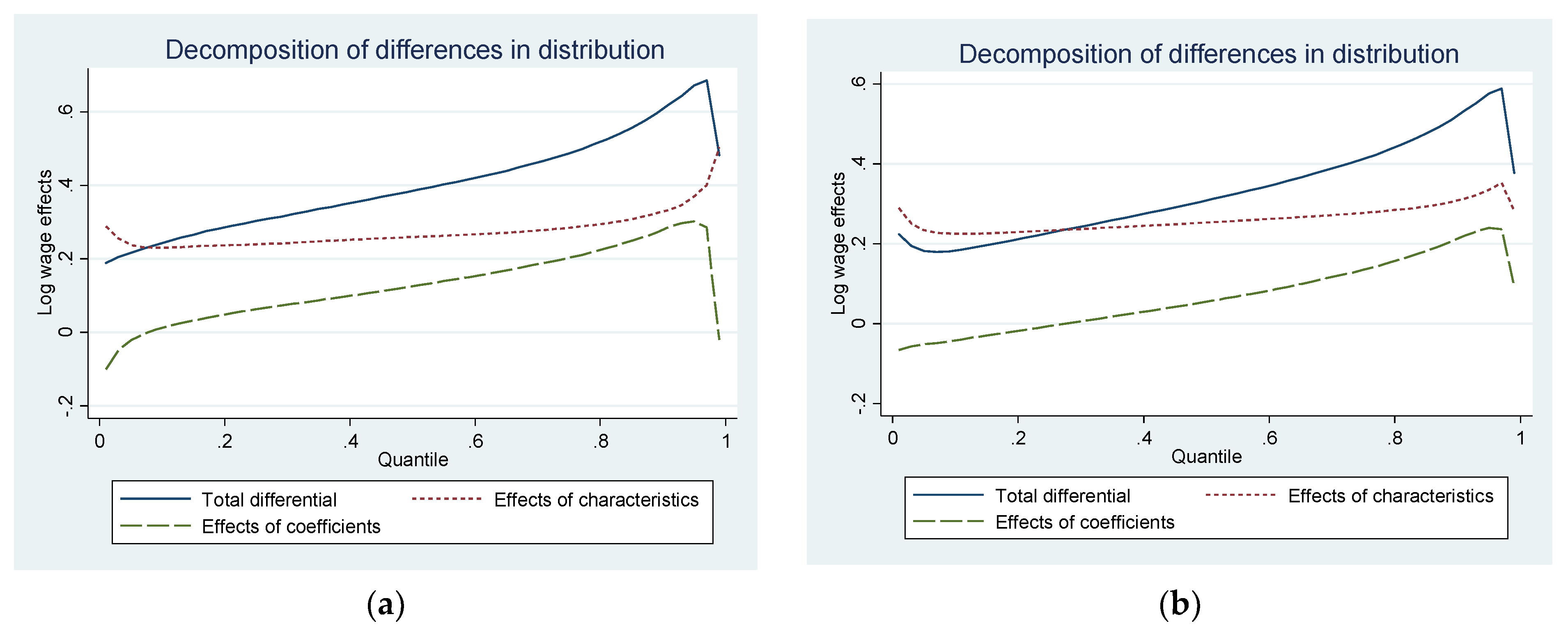
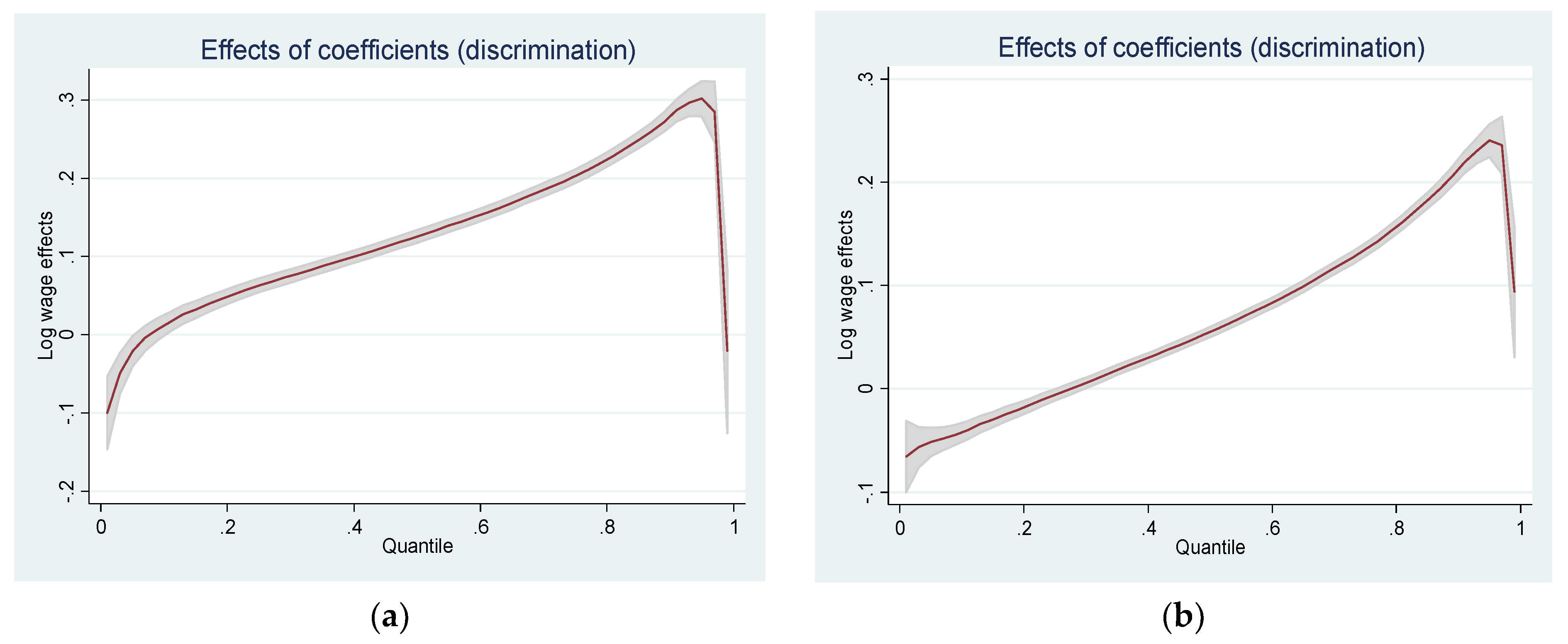
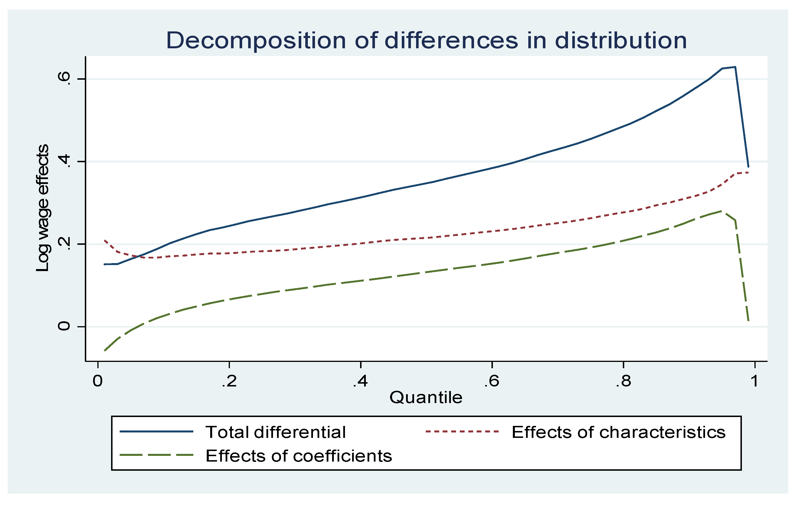
6.2. Analysis of the Results of Quantile Regression and Quantile Decomposition

The results of the quantile regression (

Table 3. Oaxaca–Blinder decomposition of wage difference between urban workers and old migrant workers.

	Total Variances		Characteristic Variances		Coefficient Variances
	Value	%	Value	%	Value	%
Education years	−0.9870	248.61	−0.2660 *** (−32.97)	90.27	−0.7210 *** (−19.17)	723.17
Work experience	−0.3750	94.46	−0.0520 *** (−6.42)	17.45	−0.3230 *** (−13.62)	323.97
Gender (M = 1)	0.0788	−19.85%	0.0195 *** (14.13)	−6.54	0.0593 *** (7.68)	−59.48
Marriage	−0.0951	23.95	0.0239 *** (12.64)	−8.02	−0.1190 *** (−6.59)	119.36
Occupation	−0.0076	1.91	−0.0476 *** (−15.63)	15.97	0.0400 (1.48)	−40.12
Industry	−0.0369	9.29	0.0167 *** (10.43)	−5.60	−0.0536 *** (−4.45)	53.76
Nature of unit ownership	0.0924	23.28	−0.000856 ** (−2.44)	−2.87	−0.1010 *** (−4.42)	101.30
Region	0.2217	−55.85	0.00871 *** (8.22)	−2.92	0.2130 *** (18.17)	−213.64
Constant term	0.9060	−228.21			0.9060 *** (11.9)	−908.73
Total variances	−0.397 *** (−55.97)	100.00	−0.298 *** (−38.77)	100.00	0.0997 *** (−10.24)	100.00

t-statistics in parentheses. ** p < 0.01, *** p < 0.001.

and

Table 4. Oaxaca–Blinder decomposition of wage difference between urban workers and new migrant workers.

	Total Variances		Characteristic Variances		Coefficient Variances
	Value	%	Value	%	Value	%
Education years	−0.4510	137.08	−0.1720 *** (−48.16)	74.78	−0.2790 *** (−7.36)	282.96
Work experience	0.1092	−33.19	−0.0228 *** (−11.06)	9.91	0.1320 *** (11.19)	−133.87
Gender (M = 1)	−0.0010	0.29	−0.0046 *** (−4.63)	1.99	0.0036 (0.56)	−3.68
Marriage	−0.0464	14.10	−0.0197 *** (−19.29)	8.57	−0.0267 ** (−2.57)	27.08
Occupation	0.0507	−15.41	−0.0241 *** (−15.15)	10.48	0.0748 *** (3.82)	−75.86
Industry	0.0082	−2.49	0.0070 *** (7.84)	−3.05	0.0012 (0.1)	−1.18
Nature of unit ownership	−0.2119	64.39	−0.0099 *** (−10.17)	4.28	−0.2020 *** (−9.22)	204.87
Region	0.1695	−51.52	0.0155 *** (15.12)	−6.74	0.1540 *** (14.68)	−156.19
Constant term	0.0425	−12.92			0.0425 (0.67)	−43.10
Total variances	0.329 *** (−50.41)	100.00	−0.23 *** (−47.46)	100.00	−0.0986 *** (−13.99)	100.00

t-statistics in parentheses. ** p < 0.01, *** p < 0.001.

) show no significant difference in the educational return of the three groups (urban workers, old migrant workers, and new migrant workers) in each quantile, which fully demonstrated the effectiveness of the OLS estimation. For urban employees, the return on work experience is insignificantly different in each quantile, and the OLS regression results are close to the 50-quantile regression results. The latter also indicates the effectiveness of the OLS regression. For gender, the increase in the quantile has an increasing effect on wages, which indicates that the gender wage difference is highly evident among urban high-income groups. The effect of having a spouse on wages also increases as the quantile grows, indicating that the premium effect of having a spouse (or marriage) is increasing. However, for the old or the new generation of migrant workers, the increase in wage quantile does not show regular changes in terms of gender and marital status.

6.3. Result Analysis of Quantile Regression and Quantile Decomposition of Wage Equation

In terms of years of education (as can be seen from

Table 5. Quantile regression results of urban workers.

	OLS	QR_10	QR_25	QR_50	QR_75	QR_90
Years of education	0.066 ***	0.071 ***	0.066 ***	0.067 ***	0.067 ***	0.063 ***
	(28.35)	(14.53)	(21.07)	(36.41)	(20.68)	(11.04)
Work experience	0.022 ***	0.028 ***	0.019 ***	0.021 ***	0.024 ***	0.027 ***
	(11.49)	(8.26)	(5.52)	(9.23)	(10.92)	(8.02)
Square of work experience	−0.001 ***	−0.001 ***	−0.000 ***	−0.000 ***	−0.001 ***	−0.001 ***
	(−10.53)	(−7.80)	(−5.51)	(−9.00)	(−9.97)	(−7.56)
Gender (M = 1)	0.171 ***	0.131 ***	0.145 ***	0.164 ***	0.193 ***	0.224 ***
	(16.54)	(10.19)	(14.3)	(14.2)	(18.64)	(12.02)
Marriage	0.090 ***	0.058 **	0.064 **	0.066 ***	0.085 ***	0.120 ***
	(6.92)	(2.68)	(3.1)	(4.97)	(6.71)	(5.84)
Occupation	Controlled	Controlled	Controlled	Controlled	Controlled	Controlled
Industry	Controlled	Controlled	Controlled	Controlled	Controlled	Controlled
Nature of unit ownership	Controlled	Controlled	Controlled	Controlled	Controlled	Controlled
Region	Controlled	Controlled	Controlled	Controlled	Controlled	Controlled
Constant term	1.937 ***	1.088 ***	1.584 ***	1.897 ***	2.270 ***	2.599 ***
	(31.64)	(8.55)	(19.77)	(30.63)	(29.18)	(17.22)
R2	0.317	0.1522	0.1752	0.2042	0.2166	0.2086
N	14,694	14,694	14,694	14,694	14,694	14,694

t-statistics in parentheses. ** p < 0.01, *** p < 0.001.

,

Table 6. Quantile regression results of old migrant workers.

	OLS	QR_10	QR_25	QR_50	QR_75	QR_90
Years of education	0.0183 ***	0.0145 ***	0.0176 ***	0.0192 ***	0.0220 ***	0.0193 ***
	(9.84)	(4.74)	(8.35)	(9.67)	(9.11)	(8.38)
Work experience	−0.0237 ***	−0.0208 ***	−0.0117 *	−0.0177 ***	−0.0321 ***	−0.0424 ***
	(−5.41)	(−3.86)	(−2.02)	(−4.09)	(−4.89)	(−4.69)
Square of work experience	0.000 **	0.000	0.000	0.000	0.000 ***	0.001 ***
	(2.91)	(1.57)	(0.09)	(1.54)	(3.37)	(3.59)
Gender (M = 1)	0.234 ***	0.224 ***	0.220 ***	0.234 ***	0.250 ***	0.233 ***
	(27.41)	(15.39)	(20.21)	(28.81)	(28.68)	(14.91)
Marriage	0.00958	0.0328	0.0336	0.0116	0.0112	−0.0142
	(0.64)	(1.09)	(1.73)	(1.04)	(0.69)	(−0.49)
Occupation	Controlled	Controlled	Controlled	Controlled	Controlled	Controlled
Industry	Controlled	Controlled	Controlled	Controlled	Controlled	Controlled
Nature of unit ownership	Controlled	Controlled	Controlled	Controlled	Controlled	Controlled
Region	Controlled	Controlled	Controlled	Controlled	Controlled	Controlled
Constant term	1.937 ***	1.088 ***	1.584 ***	1.897 ***	2.270 ***	2.599 ***
	(31.64)	(8.55)	(19.77)	(30.63)	(29.18)	(17.22)
R2	0.160	0.099	0.107	0.1137	0.1048	0.1003
N	20,997	20,997	20,997	20,997	20,997	20,997

t-statistics in parentheses * p < 0.05, ** p < 0.01, *** p < 0.001.

and

Table 7. Quantile regression results of new migrant workers.

	OLS	QR_10	QR_25	QR_50	QR_75	QR_90
Years of education	0.054 ***	0.0568 ***	0.0533 ***	0.0530 ***	0.0528 ***	0.0564 ***
	(40.88)	(27.76)	(33.27)	(49.79)	(37.47)	(30.66)
Work experience	0.0379 ***	0.0409 ***	0.0363 ***	0.0330 ***	0.0321 ***	0.0351 ***
	(19.97)	(8.79)	(18.17)	(18.09)	(12.57)	(18.14)
Square of work experience	−0.001 ***	−0.001 ***	−0.001 ***	−0.001 ***	−0.001 ***	−0.001 ***
	(−13.45)	(−6.78)	(−10.84)	(−11.95)	(−7.61)	(−10.95)
Gender (M = 1)	0.164 ***	0.135 ***	0.149 ***	0.176 ***	0.184 ***	0.201 ***
	(28.32)	(14.92)	(24.55)	(37.88)	(32.98)	(21.6)
Marriage	0.0666 ***	0.0815 ***	0.0566 ***	0.0565 ***	0.0710 ***	0.0920 ***
	(9.36)	(10.87)	(8.19)	(13.51)	(15.07)	(7.84)
Occupation	Controlled	Controlled	Controlled	Controlled	Controlled	Controlled
Industry	Controlled	Controlled	Controlled	Controlled	Controlled	Controlled
Nature of unit ownership	Controlled	Controlled	Controlled	Controlled	Controlled	Controlled
Region	Controlled	Controlled	Controlled	Controlled	Controlled	Controlled
Constant term	1.999 ***	1.107 ***	1.744 ***	2.070 ***	2.337 ***	2.624 ***
	(49.83)	(12.52)	(25.62)	(64.45)	(39.43)	(37.5)
R2	0.1926	0.1053	0.1163	0.1272	0.1337	0.1282
N	40,722	40,722	40,722	40,722	40,722	40,722

t-statistics in parentheses. *** p < 0.001.

), urban workers have the highest rate of return, followed by the new generation of migrant workers, and the old generation of migrant workers has the lowest rate of return. From the lower part of the wage distribution to the higher part of the wage distribution, the older generation of migrant workers changes greatly, while the return rate of the other two employment groups for years of education does not change much. From the perspective of work experience, urban workers still have the highest rate of return, while the wages of the older generation of migrant workers decline with the increase in work experience, which may be related to the human capital level of the older generation of migrant workers and the industry in which they are engaged. From the lower part of the wage distribution to the higher part, the older generation of migrant workers’ return on work experience changes greatly, while the return of the other two groups changes little. In terms of gender, the gender wage difference of the older generation of migrant workers is the largest, but the gender wage difference in each quartile is basically unchanged, while the gender wage difference of urban workers and the new generation of migrant workers increases with the increase in the quartile. Regarding marriage variables, whether the older generation of migrant workers get married or not has almost no impact on their wages, while there is a significant impact on urban workers and the new generation of migrant workers. Generally speaking, the impact keeps increasing with increases in the quantile of wage distribution.

On the basis of the previous decomposition, this paper applies the quantile decomposition method to decompose the wage differences at each quantile of the wage distribution between urban workers and the new and old generations of migrant workers [37,38]. To accurately measure the change trend of the wage difference caused by individual characteristics and household registration discrimination in the whole wage distribution, the quantile regression results of 1% at each interval were used to synthesize the total gender wage, characteristic, and coefficient difference curves in this study (

Table 8. Quantile decomposition results of wage difference between urban workers and old generation of migrant workers.

Quantile	Total Variances	Characteristic Variances		Coefficient Variances
		D.V.	Ratio (%)	D.V.	Ratio (%)
0.1	0.24309	0.23026	94.72%	0.01284	5.28%
0.2	0.28496	0.23662	83.04%	0.04833	16.96%
0.3	0.31788	0.2428	76.38%	0.07509	23.62%
0.4	0.35134	0.25165	71.62%	0.09969	28.38%
0.5	0.38448	0.25913	67.40%	0.12536	32.60%
0.6	0.41923	0.26634	63.53%	0.15288	36.47%
0.7	0.46215	0.2769	59.91%	0.18526	40.09%
0.8	0.51763	0.29393	56.78%	0.2237	43.22%
0.9	0.60692	0.32776	54.00%	0.27916	46.00%
0.99	0.48172	0.502211	104.25%	−0.020491	−4.25%

Note: D.V. = Difference Value.

and

Table 9. Quantile decomposition results of wage differences between urban workers and new generation of migrant workers.

Quantile	Total Variances	Characteristic Variances		Coefficient Variances
		D.V.	Ratio (%)	D.V.	Ratio (%)
0.1	0.18384	0.22538	122.60%	−0.04155	−22.60%
0.2	0.21122	0.22944	108.63%	−0.01823	−8.63%
0.3	0.24282	0.23709	97.64%	0.00573	2.36%
0.4	0.27528	0.24496	88.99%	0.03032	11.01%
0.5	0.30850	0.25340	82.14%	0.05511	17.86%
0.6	0.34534	0.26201	75.87%	0.08332	24.13%
0.7	0.38865	0.27192	69.97%	0.11673	30.03%
0.8	0.44117	0.28430	64.44%	0.15687	35.56%
0.9	0.52099	0.30804	59.13%	0.21295	40.87%

Note: D.V. = Difference Value.

; Figure 1 and Figure 2). The total difference curve shows that, regardless of group, the total difference significantly increases in the whole income distribution range with the increase in the quantile. However, high scores show a sharp decline. By contrast, the total wage difference between the old generation of migrant workers and urban workers is larger than that between the new generation of migrant workers and urban workers in all quantiles. The wage difference between urban workers and migrant workers in different positions of the wage distribution shows an asymmetric phenomenon. In terms of characteristic differences, the differences caused by individual endowments between old and new generations of migrant workers and urban workers increased with the increase in quantile. Relatively speaking, in each quantile, the difference between the old generation of migrant workers and urban workers is slightly larger than that between the new generation of migrant workers and urban workers. The trend of the coefficient difference curve is basically consistent with the total difference curve. However, the new generation of migrant workers and urban workers in the low quantile demonstrates more typical anti-discriminatory phenomena. The generation of migrant workers suffered more discrimination than the new generation at any given quantile.

Although there have been in-depth studies on the intergenerational differences between migrant workers in the academic world, the literature has typically neglected the intergenerational differences in household registration discrimination. With the development of the economy and society, there has been an obvious intergenerational differentiation between migrant workers, so there may be a large intergenerational difference in the degree of wage discrimination for different migrant workers. Regarding the new generation of migrant workers, they may have a stronger sense of safeguarding their rights. In the situation of increasingly fierce labor conflicts, it is of great practical significance to study wage discrimination between urban and rural labor from the perspective of generational differences. Based on this, the innovation of this paper mainly lies in the new perspective it offers of generational differences between the new two generations of migrant workers wage discrimination, and in its in-depth analysis of these differences.

6.4. Robustness Test

To ensure the robustness of the decomposition results of inter-generational wage differences, this paper decomposes the wage differences between urban workers and migrant workers born in the 1970s and urban workers and migrant workers born in the 1980s.

Table 10. Decomposition of quantile of wage difference between urban workers and the old generation of migrant workers.

Quantile	Total Variances	Characteristic Variances		Coefficient Variances
		D.V.	Ratio (%)	D.V.	Ratio (%)
0.1	0.19562	0.16810	85.93	0.02753	14.07
0.2	0.24414	0.17820	72.99	0.06595	27.01
0.3	0.27826	0.18756	67.40	0.09071	32.60
0.4	0.31350	0.20189	64.40	0.11162	35.60
0.5	0.34745	0.21537	61.99	0.13208	38.01
0.6	0.38423	0.23134	60.21	0.15289	39.79
0.7	0.43003	0.25112	58.40	0.17891	41.60
0.8	0.48561	0.27708	57.06	0.20853	42.94
0.9	0.56847	0.31308	55.07	0.25539	44.93

and

Table 11. Decomposition of quantile of wage difference between urban workers and the new generation of migrant workers.

Quantile	Total Variances	Characteristic Variances		Coefficient Variances
		D.V.	Ratio (%)	D.V.	Ratio (%)
0.1	0.09246	0.12111	130.99	−0.02865	−30.99
0.2	0.12734	0.13136	103.16	−0.00402	−3.16
0.3	0.16036	0.14101	87.93	0.01935	12.07
0.4	0.19230	0.14976	77.88	0.04255	22.12
0.5	0.22498	0.15899	70.67	0.06599	29.33
0.6	0.26147	0.17041	65.17	0.09106	34.83
0.7	0.30275	0.18205	60.13	0.12070	39.87
0.8	0.35244	0.19794	56.16	0.15450	43.84
0.9	0.42399	0.22284	52.56	0.20115	47.44

, Figure 3 and Figure 4 show the specific decomposition results. From the perspective of the total wage difference curve and the characteristic curve of urban workers and migrant workers, the conclusion is completely consistent with the previous conclusion. The robustness test shows that, overall, a larger wage difference exists between urban workers and the older generation of migrant workers. In addition, the older generation of migrant workers suffers from a higher degree of discrimination, thus verifying the robustness of the previous conclusion.

7. Conclusions and Policy Recommendations

7.1. Theoretical Conclusions

This study used the China Migrants Dynamic Survey. The wage difference between new- and old-generation migrant and urban workers was found using the Oaxaca–Blinder method and the quantile decomposition methods. When estimating the wage equation, the correlation between education and the missing variable “ability” leads to the endogeneity problem. In general, more able people are likely to have higher degrees and higher incomes, thus omitting the “ability” variable, which overestimates the effect of education on wages. Therefore, it is important to find appropriate instrumental variables in subsequent studies. In general, through the empirical research, the following conclusions can be drawn in this paper.

First, overall, an obvious wage gap exists between the two generations of migrant and urban workers. However, compared with the old generation of migrant workers, the wage gap between the new generation of migrant and urban workers has been narrowed. Compared with the old generation of migrant workers, the differences in individual characteristics and coefficient between the new generation of migrant and urban workers have been reduced. This finding indicates that the new generation of migrant workers have few differences in terms of individual qualities and household registration discrimination.

Second, from the perspective of wage distribution, the old generation of migrant and urban workers demonstrate anti-discriminatory phenomena at low and extremely high scores, whereas the new generation of migrant workers and urban workers only show anti-discriminatory phenomena at low scores. The urban–rural wage difference tends to increase with the increase in wage distribution from low scores to high scores. Overall, the variation trend of the discrimination coefficient of the two generations of migrant workers is similar. However, compared with the new generation of migrant workers, the old generation of migrant workers suffers from more serious discrimination.

Third, in terms of the various influencing factors, the main reasons for the wage difference between urban and rural labor forces are the educational level and education rate of return. Compared with the new generation of migrant workers, the old generation of migrant and urban workers show a greater difference in the rate of return on education. According to the overall decomposition result of wage difference, the two methods of wage difference decomposition reach the same conclusion.

7.2. Practical Conclusions

Based on the above conclusions, although household registration discrimination is no longer the main factor for the wage and income difference between urban and rural labor forces, household registration remains the main reason for the individual characteristic differences between migrant and urban workers in education investment. Given the huge gap between urban and rural economic development in China, investment in human capital, such as education and skill training in rural areas, is far less than that in urban areas. This phenomenon leads to differences in the other individual characteristics. The changes in the wage differences between the two generations of migrant and urban workers show that the difference in educational level between the new generation of migrant and urban workers is smaller than that with the old generation of migrant workers. Consequently, the wage difference between the new generation of migrant and urban workers is also small. To promote the full protection of the legitimate rights and interests of migrant workers, the government must first eliminate household registration discrimination and create a highly equitable employment environment. Moreover, the government should vigorously promote the equalization of urban and rural education services, specifically improving the human capital level of migrant workers through an improved education and training to narrow the wage gap between urban and rural areas.

The wage differences in the labor market studied in this paper only includes the employment wage and business income. Wage income includes individual wages, bonuses, overtime pay, allowances, and the equivalent funds of the unit. It does not include rewards, social security, the variety of welfare, and other forms of income, which may underestimate the wage differences between urban workers and migrant workers. In the follow-up research, further subdividing the age group into five years is necessary, to comprehensively investigate the wage differences between the urban and rural labor forces of different age groups.

7.3. Limitations and Future Research Line

The main inconvenience of the Oaxaca–Blinder approach is that it only measures the discrimination in the labor market. If differences in access to endowments are rewarded in the labor market, for example, if women have worse access to higher education than men or if, ceteris paribus, men are more likely to work than women, then the Oaxaca–Blinder standard approach tends to underestimate the degree of discrimination [40].

Furthermore, according to Atal, Ñopo and Winder (2009) although the decomposition Blinder–Oaxaca is the approach that is most applied in research on wage differentials, it has three notable flaws: First, the decomposition only provides information about the average wage gap, omitting the different distributions of this gap among individuals in the same group [41]. Secondly, the authors note that the relationship between characteristics and wages was observed to not necessarily be linear and found that recent data violate fundamental implications of the Mincer model, which is the key input of the decompositions. Finally, the decomposition does not restrict the analysis to comparable individuals, which can lead to an upward bias of the component associated with discrimination.

To close, in the follow-up study, we need to subdivide the age groups into five years, to more comprehensively investigate the wage differences between urban and rural labor in different age groups. The time trend of wage difference is also very important, so the follow-up analysis will examine the wage differences between urban and rural areas in different years. Finally, the research done in this paper is essentially a problem of income inequality among workers, but due to the limitations of economic theory and mathematical measurement methods, there are still many problems in the actual research. The research conclusion should be combined with further analysis in China, to draw the conclusion that is closest to the real situation of the labor market.

References

1. Morikawa, M. A comparison of the wage structure between the public and private sectors in Japan. J. Jpn. Int. Econ. 2016, 39, 73–90. [Google Scholar] [CrossRef] [Green Version]
2. Wu, X. The research of yield on human capital of rural migrant workers. Youth Stud. 2009, 4, 66–74. [Google Scholar]
3. Wang, M. Wage difference in the transition period: A quantitative analysis of discrimination. Quant. Econ. 2003, 28, 94–98. [Google Scholar]
4. Hu, B. Research on wage difference between urban and rural laborers: Based on the theory of compensatory wage difference. East China Econ. Manag. 2016, 10, 107–115. [Google Scholar]
5. Wang, H.; Chen, Y. Quantile regression analysis of the difference of salary differences among urban migrants. World Econ. Pap. 2010, 4, 64–77. [Google Scholar]
6. Zhang, C. Analysis of the citizenization of migrant workers’ salary and its influencing factors from the intergenerational perspective. Econ. Issues 2018, 3, 99–103. [Google Scholar]
7. Deutschmann, C. Labour market segmentation and wage dynamics. Manag. Decis. Econ. 2015, 2, 145–159. [Google Scholar] [CrossRef]
8. Démurger, S.; Hou, Y.; Yang, W. Forest management policies and resource balance in china: An assessment of the current situation. J. Environ. Dev. 2007, 18, 17–41. [Google Scholar] [CrossRef] [Green Version]
9. Mincer, J. Human capital and the labor market: A review of current research. Educ. Res. 1989, 18 4, 27–34. [Google Scholar] [CrossRef]
10. Démurger, S.; Xu, H. Return migrants: The rise of new entrepreneurs in rural China. World Dev. 2011, 39, 1847–1861. [Google Scholar] [CrossRef]
11. Du, L.; Peng, J. Urban differences in educational return rate. Chin. Popul. Sci. 2010, 20, 85–94. [Google Scholar]
12. Xie, S.; Yao, X. Econometric analysis of migrant workers’ salary discrimination. Chin. Rural Econ. 2006, 26, 49–55. [Google Scholar]
13. Deng, Q. Income differences between urban residents and floating population: Decomposition based on method. Chin. Popul. Sci. 2007, 2, 8–16. [Google Scholar]
14. Yu, X.; Chen, X. Empirical research on the effect of the household registration system evolvement on labor market segmentation in China: From dual perspectives of employment opportunities and wage gap. Econ. Res. 2012, 12, 97–110. [Google Scholar]
15. Ge, Y.; Zeng, X. The influence of market discrimination on the gender wage gap in urban areas. Econ. Res. 2011, 18, 45–56. [Google Scholar]
16. Xing, C. The income gap between migrant workers and urban workers. Manag. World 2008, 6, 55–64. [Google Scholar]
17. Guo, F.; Zhang, S. The influence of education and household registration discrimination on the difference of salary between urban workers and migrant workers. Agric. Econ. Issues 2011, 26, 35–42. [Google Scholar]
18. Kuang, L.; Liu, L. Discrimination against rural-to-urban migrants: The role of the Hukou System in China. PLoS ONE 2012, 7, e46932. [Google Scholar] [CrossRef] [PubMed] [Green Version]
19. Meng, F.; Wan, H.; Wu, S. Ownership division, household registration discrimination and intergenerational urban-rural wage differences. Contemp. Financ. Econ. 2019, 6, 13–25. [Google Scholar]
20. Zhu, R. Wage differentials between urban residents and rural migrants in urban China during 2002–2007: A distributional analysis. China Econ. Rev. 2016, 37, 2–14. [Google Scholar] [CrossRef]
21. Li, X.; Yao, Y. A study of the paradox of simultaneous expansion of labor force shift and wage gap: From the perspective of market segmentation. Contemp. Financ. Econ. 2012, 4, 5–12. [Google Scholar]
22. Islam, N.; Yokota, K. Lewis growth model and china’s industrialization. Asian Econ. J. 2008, 22, 359–396. [Google Scholar] [CrossRef]
23. Bu, N.; Kong, H.; Yi, S. Research on the Differences in Household Registration Wages from the Perspective of Intergenerational. Stat. Decis. 2020, 1, 77–80. [Google Scholar]
24. Liu, A.Y.C. Segregated and not equal? Occupation, earnings gap between urban residents and rural migrants in Vietnam. Int. J. Manpow. 2019, 40, 36–55. [Google Scholar] [CrossRef]
25. Le, B.D.; Tran, G.L.; Nguyen, T.P.T. Social Protection for Rural-Urban Migrants in Vietnam: Current Situation, Challenges, and Opportunities; CSP Research Report No. 8; Institute for Social Development Studies: Hanoi, Vietnam, 2011. [Google Scholar]
26. Chan, K.W. The household registration system and migrant labor in China:notes on a dabate. Publ. Dev. Rev. 2010, 36, 357–364. [Google Scholar] [CrossRef] [PubMed]
27. Liang, L.; Chen, Q.Y.; Wang, R.Y. Household registration reform, labour mobility and optimization of the urban hierarchy. Soc. Sci. 2015, 36, 131–151. [Google Scholar]
28. Franceschini, I.; Siu, K.; Chan, A. The “rights awakening” of Chinese migrant workers: Beyond the generational perspective. Crit. Asian Stud. 2016, 48, 422–442. [Google Scholar] [CrossRef]
29. Chan, K.W. The global financial crisis and migrant workers in china: ‘there is no future as a laborer; returning to the village has no meaning’. Int. J. Urban Reg. Res. 2010, 34, 659–677. [Google Scholar] [CrossRef]
30. Chan, C.K. Community-based organizations for migrant workers’ rights: The emergence of labour NGOs in China. Commun. Dev. J. 2013, 48, 6–22. [Google Scholar] [CrossRef]
31. Lv, X.; Yao, X. Research on the intergenerational differences between migrant workers—Based on wage determination and willingness of staying in the city. Res. Econ. Manag. 2014, 9, 32–42. [Google Scholar]
32. Zhang, D.D.; Meng, X.; Wang, D.W. The Dynamic Change in Wage Gap between Urban Residents and Rural Migrants in Chinese Cities. 2010. Available online: https://papers.ssrn.com/sol3/papers.cfm?abstract_id=1706289 (accessed on 20 October 2021).
33. Jin, S.F.; Wu, Y.T.; Cheng, M.D. An empirical analysis of the wage difference of the new generation of migrant workers: Based on the survey data of Chengdu. Rural Econ. Sci. Technol. 2018, 29, 126–129. [Google Scholar]
34. Wang, M. The consumption level and consumption structure of the new generation of migrant workers: A comparison with the previous generation of migrant workers. J. Labor Econ. 2017, 5, 107–126. [Google Scholar]
35. Glaser, G.; Andersson, R.; Musterd, S.; Kauppinen, T.M. Does neighborhood income mix affect earnings of adults? new evidence from sweden. J. Urban Econ. 2008, 63, 858–870. [Google Scholar]
36. Melly, B. Decomposition of differences in distribution using quantile regression. Labour Econ. 2005, 12, 577–590. [Google Scholar] [CrossRef] [Green Version]
37. Oaxaca, R. Male–female differentials in urban labor markets. Int. Econ. Rev. 1973, 14, 693–709. [Google Scholar] [CrossRef]
38. Machado, J.A.F.; Mata, J. Counterfactual decomposition of changes in wage distributions using quantile regression. J. Appl. Econom. 2010, 20, 445–465. [Google Scholar] [CrossRef] [Green Version]
39. Melly, B. Estimation of Counterfactual Distributions Using Quantile Regression. Ph.D. Thesis, University of St. Gallen, St. Gallen, Switzerland, 2006. [Google Scholar]
40. Madden, D. Towards a Broader Explanation of Male-Female Wage Differences. Cent. Econ. Res. 1999, 99, 11–15. [Google Scholar] [CrossRef] [Green Version]
41. Atal, J.P.; Nopo, H.; Winder, N. New Century, Old Disparities: Gender and Ethnic Wage Gaps in Latin America; IDB Working Paper IDB-WP-109; Department of Research and Chief Economist, Inter-American Development Bank: Washington, DC, USA, 2009. [Google Scholar]
Figure 1. Quantile decomposition of wage differences between urban workers and different migrant worker groups. Note: D.V. = Difference Value. (a) Urban workers and old generation of migrant workers; (b) Urban workers and new generation of migrant workers.
Sustainability 13 11835 g001
Figure 2. Coefficient of household registration discrimination between urban workers and different migrant workers’ groups. (a) Urban workers and old generation of migrant workers; (b) Urban workers and new generation of migrant work-ers.
Sustainability 13 11835 g002
Figure 3. Decomposition of quantile of wage difference between the old generation of migrant workers and urban workers.
Sustainability 13 11835 g003
Figure 4. Decomposition of quantile of wage difference between the new generation of migrant workers and urban workers.
Sustainability 13 11835 g004