Assessing Land Cover and Ecological Quality Changes under the New-Type Urbanization from Multi-Source Remote Sensing

Abstract

The traditional rapid urbanization process is the result of a strong focus on economic development, while its ecological and environmental aspects are less focused upon. The “new-type urbanization” (NTU) concept considers ecological conservation during the urbanization process. The different impacts of the two processes on regional ecological environment evolutions remain insufficiently investigated and still draw significant attention from urban planners and land managers when formulating proper land use policies. Thus, this study was designed to fill the gap by evaluating and comparing different effects of the traditional urbanization and NTU on urban land cover (LC) and ecological quality changes in the Jiangbei New Area, Nanjing, China. We first established a LC database using an object-oriented classification of multi-source high-resolution satellite images. Next, we quantified changes in ecological quality using the remote sensing ecological index (RSEI) model. Subsequently, spatial auto-correlation analysis was conducted to detect the clustering trend of the changing ecological quality in the study area over time. The results showed that the overall accuracy of the LC maps was 90.75% in 2009, 91.75% in 2015, and 92.04% in 2019. The average RSEI values of the study area were 0.583, 0.559, and 0.579, respectively. The spatial auto-correlation analysis indicated a strong positive correlation between the ecological qualities. However, the spatial distribution changed slightly from a clustered trend to a more random and dispersed trend as the Moran’s I decreased. The observed changes are attributed to the strict implementation of ecological conservation and restoration policies by the local government in the NTU process, as well as an increased residents’ awareness of protecting natural resources, indicating that the traditional urbanization has a stronger negative disturbance on regional ecological conditions than NTU. The proposed evaluation method can be applied to other similar regions for sustainable urban management.

1. Introduction

Land cover (LC) change is a dynamic process driven by anthropogenic and natural factors and plays a pivotal role in global environmental change studies [1], ecological deterioration assessment [2], risk evaluation of biodiversity loss [3], and the transformation of natural LC into impervious surfaces. LC change caused by traditional urbanization has a profound impact on the structure, function, and ecological process of urban ecosystems [4], leading to ecological and environmental problems, such as a sharp reduction in cultivated land, increased congestion, water logging, the heat island effect [5], and environmental pollution. “New-type urbanization” (NTU), which was first proposed at the Central Economic Working Conference of China in 2012, is defined as intensive, intelligent, green, and low-carbon urbanization for eco-friendly urban development [6,7,8]. These two types of urbanization processes differ in the land use patterns, change speeds, and directions. However, due to technical limitations and management cost of urban construction, few spatio-temporally explicit assessments have been conducted to indicate the effectiveness and lessons to be learned from the two types of urbanization processes. In addition, few studies have jointly considered changes in LC and ecological quality simultaneously [9,10,11].

The Nanjing Jiangbei New Area (JBNA) was designated as the 13th National New Area in China by the Central Government of China in 2015 as a prototype because the area experienced both traditional urbanization and NTU during the past 10 years [4]. As an urban fringe of Nanjing city, the JBNA has lagged behind the development of the main city area on the opposite bank of the Yangtze River since before 2015. Due to its unique location at the intersection between the Yangtze River Economic Belt and the Eastern Coastal Economic Belt of China, the JBNA is a vital gateway of the Yangtze River Delta to drive the development of the middle and upper reaches of the Yangtze River [12]. Thus, an assessment of the impacts of the two types of urbanization processes on the changes in LC and ecological quality in the JBNA pioneer area will have important practical significance for governmental departments to take active countermeasures to achieve the goals of environmental protection and sustainable economic and social development, which are NTU requirements.

Unlike other state-level new areas, the JBNA has abundant natural resources, such as the Laoshan National Forest Park, Lvshuiwan Wetland Park, Longwang Mountain Forest Farm, Chu River, and Foshou Lake, most of which are within the scope of the ecological red line protection area [13]. Since the area was not appropriately developed to improve regional livability, the landscape function and green value of the area have not been adequately evaluated. To balance the conflict between resource protection and urban development, the JBNA Development Agenda, which was approved by the Central Government of China, states that the JBNA will upgrade its industrial structure to become environmentally friendly and innovatively smart [14]. The JBNA will strictly follow the 13th Five-Year Plan for Ecological Environment Protection and the Plan for the Construction of Ecological Civilization of Jiangsu Province (2013–2022) to optimize the layout of urban spaces and the allocation of regional ecological resources to set an example for NTU [14]. However, five years after the designation of the JBNA, its effectiveness remains unclear. Specifically, a spatially explicit assessment of whether the JBNA construction process followed the above-mentioned administrative policies and guidelines has not been conducted.

Traditional assessments of changes in LC and ecological quality highly depend on extensive field visits and measurements. These assessments are time consuming, labor-intensive, costly, and difficult to implement in large regions [15]. Remote sensing imagery contains abundant spectral and textural information, with excellent temporal and spatial resolutions and broad coverage [16], minimizing the limitations of traditional methods. High-resolution images have substantial advantages over medium- or coarse-resolution satellite images in terms of details, including rich landscape characteristics, detailed information on the size and shape of surface targets, and the spatial relationships between neighboring objects. Thus, high-resolution imagery provides new opportunities for highly accurate and detailed LC mapping at regional scales [17,18,19]. Object-oriented image analysis has attracted increasing recognition among the remote sensing community and has been increasingly used for LC mapping using high-resolution satellite images. The mapping accuracy of object-oriented image analysis approaches that of human visual interpretation and is often higher than that of per-pixel classifiers [20,21]. The object-oriented classification method considers the spectral, geometric, texture, topological, and spatial characteristics [22], reducing the salt-and-pepper noise of traditional pixel-based classifications [23]. Recently, deep learning has become a hotspot in LC classification, and its most representative and discriminative features are learned end to end, hierarchically [24]. In LC classification, the deep convolutional neural network (CNN) and its derivative networks have received the greatest attention [25,26]. These networks offer great potential to extract high-level spatial features due to their hierarchical nature with multiple levels of abstraction [27]. However, the blurred object boundaries and geometric distortion, as well as huge computational redundancy, highly restrict the potential application of the existing CNN models including both patch-based and pixel-level approaches. Thus, we chose an object-oriented method rather than multiple deep learning models to cope with the LC classification in the study area with high-resolution images [28].

Additionally, remote sensing is an effective method to assess regional ecological change to obtain a better understanding of ecological patterns and processes [29,30,31,32]. A single remote sensing-based ecological index, such as the normalized difference vegetation index (NDVI), does not comprehensively reflect the conditions of entire ecosystems due to the ecological complexity [33]. Thus, an integrated index is required for comprehensively and objectively assessing complex urban ecosystems. The remote sensing ecological index (RSEI) was first proposed by Xu et al. (2013) [34]. It has four indicators (greenness, wetness, dryness, and heat) to reflect the quality of an ecosystem and its changes driven by human activities. The RSEI is established typically by conducting a principal component analysis (PCA) of the four indicators [35,36]. The RSEI has proven effective for the change analysis of ecological quality in areas prone to soil erosion, urban areas [37], and for monitoring ecological quality changes in 35 major Chinese cities [38]. However, few studies have sought to elucidate the causal relationships between the spatio-temporal LC patterns and ecological quality changes. Ariken et al. (2020) found the current sluggish urbanization and ecological environment coupling in the urban areas of the Yanqi Basin showed a moderate imbalanced relationship, indicating that urbanization development has a certain interference effect on the ecological environment [39]. Shan et al. (2019) argued that the land consolidation project caused persistent disturbance to ecological environmental quality, and there was a lag for restoration for more than 5 years [40]. Hang et al. (2020) discovered that the ecological conditions in the main urban districts of Nanjing improved, whereas the ecological conditions of new urban districts and suburban town centers deteriorated along the urban expansion. The infrastructure construction and real estate development were the main factors [37]. Xu et al. (2018) revealed quantitative relationships between three land covers (impervious surface, vegetation, water) and RSEI, and the relationship between population growth and impervious surface increase was helpful for urban planners to predict ecological effect of their new plan works [5]. Knowledge of these causes is crucial for understanding the underlying change mechanisms of ecological environments to facilitate the design of practical measures of NTU for protecting and restoring ecological environments.

The major objectives of the current work were as follows: (1) to assess the implementation effectiveness and its timely impact on land cover and landscape qualities of NTU in the JBNA, which experienced traditional urbanization and NTU processes by analyzing the LC and ecological quality changes from 2009 to 2019; and (2) to explore the socioeconomic drivers responsible for the observed changes to learn lessons from past urban development to provide information for NTU implementation in similar regions.

2. Materials and Methods

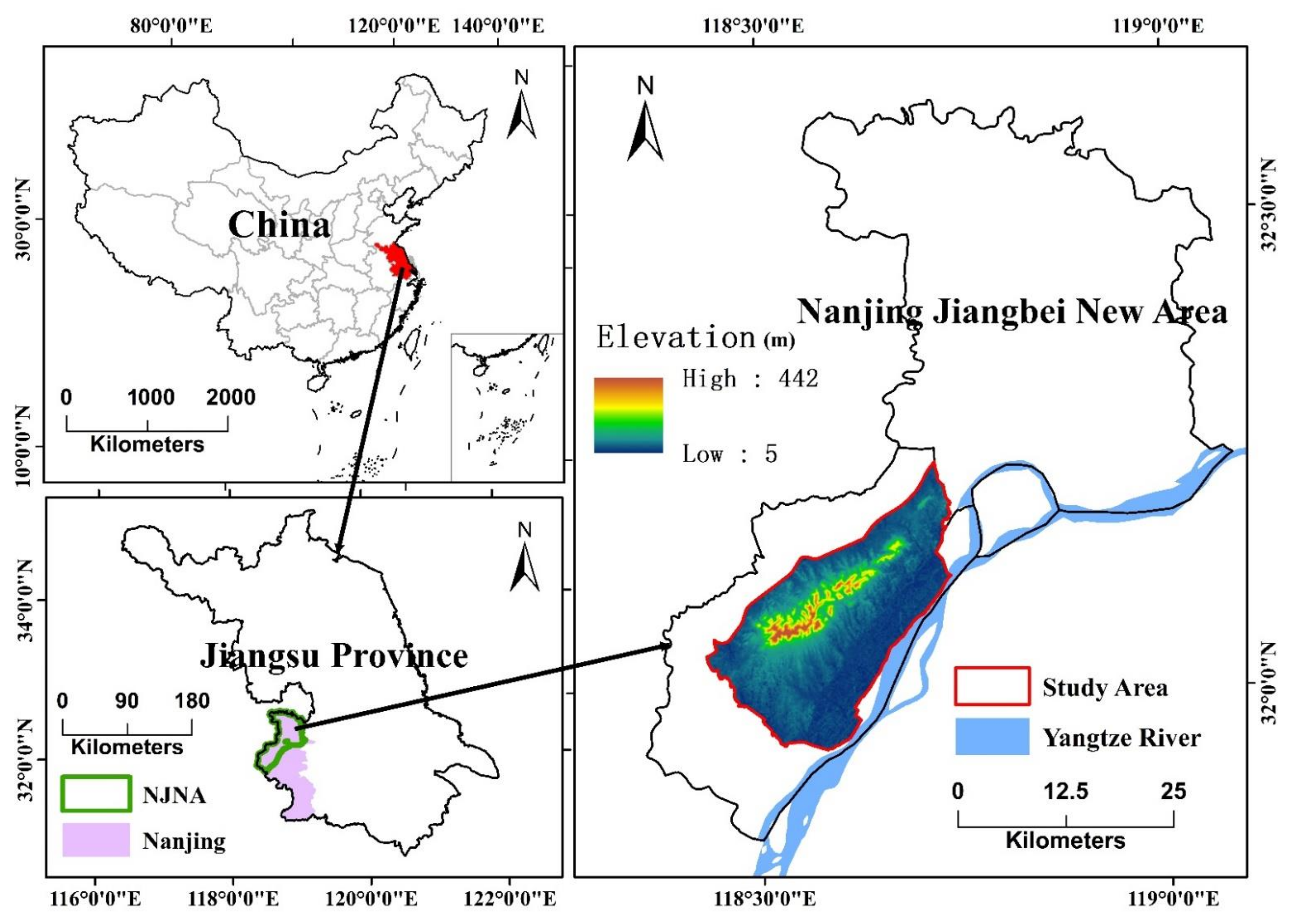
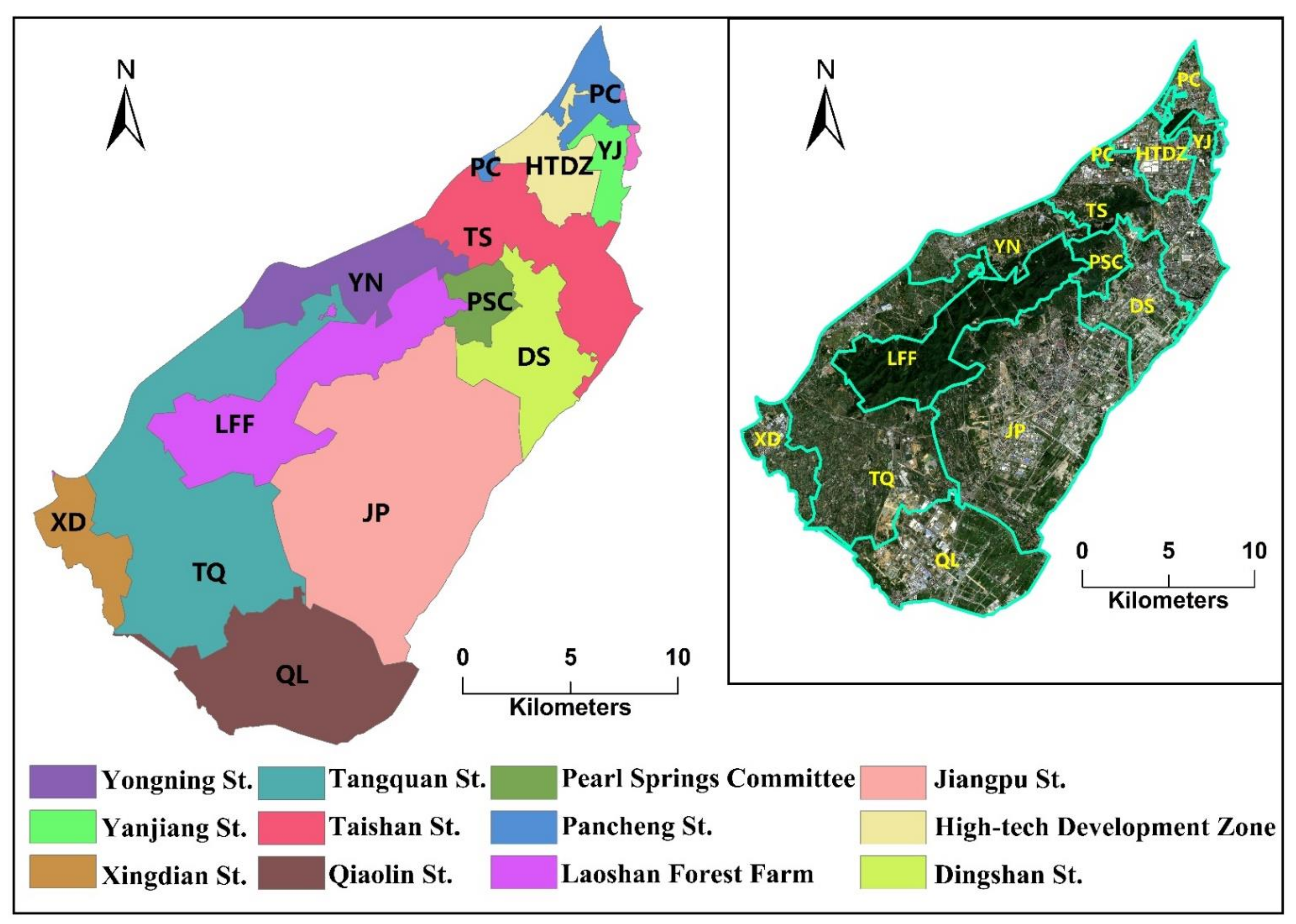
2.1. Study Area

We confined our analysis to the core region of the JBNA to achieve spatial consistency of the remote sensing images acquired in the three years (Figure 1). The study area extends from 118°25′ E, 31°56′ N to 118°45′ E, 32°15′ N, with a total area of 437.256 km² and is located in the Pukou District along the Yangtze River (Figure 1). The study area contains the core development area (e.g., Pukou New City core zone, high-tech development zone, Qiaolin New City, Nanjing Chemical Industry Park) and an ecological protection zone (e.g., Laoshan National Forest Park, Lvshuiwan Wetland Park) of JBNA (Figure 2). Among them, Laoshan National Forest Park is the largest national forest park in Jiangsu; it has more than 90% forest cover and plays a vital role in the urban ecosystem (Figure 2).

The study area has a subtropical monsoon climate with four distinct seasons and an annual mean temperature of about 15.3 °C. The elevation ranges from 5 to 442 m above sea level. The average annual precipitation is 1020 mm, and 70% of the annual precipitation falls in the rainy season from June to July.

2.2. Data Resources and Image Pre-Processing

In this study, three types of high-resolution remote sensing images (RapidEye (25 June 2009), Gaofen-1 (GF-1) WFV (3 August 2015), and Sentinel-2A (19 September 2019)) were collected to support the generation of high spatial resolution LC datasets. The Sentinel-2A top of atmosphere reflectance product obtained from the European Space Agency (ESA) was atmospherically corrected using the Sen2cor plug-in to derive land surface reflectance data [41]. The RapidEye and GF-1 WFV images were atmospherically corrected using the FLAASH module in the ENVI 5.3. We used the RapidEye image as the base image and co-registered the GF-1 WFV and Sentinel-2A images using a quadratic polynomial and the nearest neighbor interpolation method. Twelve ground control points evenly distributed throughout the entire study area were identified for the registration. The RMSE values of the co-registrations were less than 0.5 pixels, and the WGS_1984_UTM_Zone_50N projection was specified. The corrected images were used to map the LC in the study area.

Additionally, we downloaded high-quality Landsat Level-2 science products, which were atmospherically corrected and orthorectified by the USGS EROS data center, to support our analysis of the ecological quality evaluation using the RSEI model. Specifically, temporally consistent Landsat 5 TM (13 June 2009) and Landsat 8 OLI/TIRS (14 June 2015/13 September 2019) level 2 images with a cloud cover of less than 5% were obtained to determine the ecological quality. The detailed information of the images is summarized in

Table 1. Description of the satellite images used in the analysis.

Satellites	Acquisition Date	Bands	Spatial Resolution (Pan/Multi-Spectral, m)
RapidEye	25 Jun 2009	Blue, Green, Red, Red edge, Near infrared	none, 5
GF-1 WFV4	3 Aug 2015	Blue, Green, Red, Near infrared	none, 16
Sentinel-2A	19 Sep 2019	Blue, Green, Red, Red edge, Near infrared, Shortwave infrared	none, 10
Landsat 5 TM	13 Jun 2009	Blue, Green, Red, Near infrared, Shortwave infrared, Longwave infrared	none, 30
Landsat 8 OLI/TIRS	14 Jun 2015 13 Sep 2019	Blue, Green, Red, Near infrared, Shortwave infrared, Longwave infrared	15, 30

.

2.3. Object-Oriented Land Cover Classification and Accuracy Assessment

We performed a multi-scale segmentation and followed by the regression tree (CART) classification in eCognition 8.7 based on the segmented images to generate LC classifications in 2009, 2015, and 2019. The image features used by the classifier included the pre-processed original bands and their derivatives, such as the NDVI, modified normalized difference water index (MNDWI), elevation, and slope. The LC types in the study area were pre-defined as cropland, forest, grassland, water body, urban land, and unused land according to the National Land Classification System and considering the conditions of the study region [42].

The multi-scale segmentation method is a region-merging algorithm that merges adjacent pixels or segmented objects from bottom level to top level on the premise of ensuring the minimum homogeneity between pixels and the maximum heterogeneity between segmented objects. In eCognition 8.7, the homogeneity criteria contain “Color”, “Shape” “Compactness”, and “Smoothness”. The weights of “Color” and “Shape” add up to 1, the same as “Compactness” and “Smoothness”. Setting as much “Color” and necessary “Shape” as possible can make the segmented objects’ boundaries smooth and compact to improve the accuracy of classification.

Since the ability to describe LC differs in the three types of high-resolution images, the segmentation parameters had to be determined appropriately. The control variables method was adopted to determine the “Shape” and “Compactness” in eCognition 8.7 to achieve the optimal segmentation [23]. Then we used the Estimation of Scale Parameter (ESP2) tool and visual assessment to determine the validity of the automatic selection of the optimal segmentation scale parameters [43,44].

After image segmentation, we used field investigation data, Google Earth images, and Forest Management Inventory data (2017) as references to collect sample polygons of the segmented objects in eCognition 8.7 as training samples, ensuring that each polygon only contained one LC type. Subsequently, the Feature Space Optimization (FSO) module was used to optimize the features of interest, followed by implementing the CART algorithm to classify the segmented objects using the spectral, shape, texture, and topological features derived from the training samples.

The CART algorithm divides the training dataset into test variables and target variables. The cyclic analysis of these two types of variables creates a decision tree consisting of multiple binary trees. After calculating the spectral, shape, texture, and other features of the segmented objects, the class assignment, the features, and the thresholds of the features were automatically determined by the CART algorithm. CART tree uses the Gini coefficient, which is commonly used in economic studies, as the criteria for selecting the optimum classification features and feature thresholds; the Gini index is defined as follows:

$$Gin{i}_{Index}=1-{\displaystyle \sum }_i^I{p}^2\left(i/h\right)$$

(1)

$$p\left(i/h\right)=n_i\left(h\right)/n\left(h\right)$$

(2)

$${\displaystyle \sum }_i^{I}p\left(i/h\right)=1$$

(3)

where $p\left(i/h\right)$ represents the probability that a sample drawn randomly from the training sample set belongs to the j category when one of its test variables is $h$. $n_i\left(h\right)$ represents the number of samples belonging to the$i$ category when the test variable value is $h$ in the training sample; $n\left(h\right)$represents the number of all samples in the training sample when the test variable value is $h$.

The preliminary object-oriented classification results might contain errors; thus, visual interpretation and on-screen editing or correction were used to improve the classification accuracy. Subsequently, the final classification results were merged, the boundaries were smoothed, and the classifications were rasterized to 5 m spatial resolution LC maps.

Error matrices and overall accuracy indices were derived to discriminate genuine LC changes from possible spurious changes resulting from classification errors. The temporally corresponding Google Earth images, Forest Management Inventory data (2017), and field investigation data were used as references, and 400 random points were generated in the classified images. The real LC classes were ascertained through on-site investigation data and visual interpretation of the Google Earth images for the three periods, and the results were compared with the classifications to construct three confusion matrices. The overall accuracy and Kappa coefficient for each year were derived to represent the reliability of the classifications [45].

2.4. Land Cover Change Analysis

An LC transition matrix that intuitively shows the change in the area and direction of LC types was created for the two time periods of 2009–2015 and 2015–2019. The annual change rate (ACR) was used to quantify the LC change; it refers to the change rate of an LC type in a certain time and area [46,47]. It has the advantage of describing the regional differences in LC changes and predicting future LC change trends. The ACR is computed as follows:

$$\mathrm{ACR}=\frac{{\mathrm{U}}_{\mathrm{n}+\mathrm{t}}-{\mathrm{U}}_{\mathrm{n}}}{{\mathrm{U}}_{\mathrm{n}}}\times \frac{1}{\mathrm{T}}\times 100\%$$

(4)

where ${\mathrm{U}}_{\mathrm{n}}$ and ${\mathrm{U}}_{\mathrm{n}+\mathrm{t}}$ are the area of the LC type at the beginning and end of the time period, respectively, and T is the number of years in the time period.

2.5. RSEI Model

The RSEI can effectively and objectively evaluate regional ecological quality without requiring weights and threshold settings (Xu et al., 2013) [29]. It is defined as follows:

$$\mathrm{RSEI}=f\left(\mathrm{NDVI},\mathrm{Wet},\mathrm{LST},\mathrm{NDSI}\right)$$

(5)

Here, the inputs of the transformation function $f$ include the NDVI, the wetness from the Tasseled Cap (TC) transformation, the land surface temperature (LST), and the normalized difference built-up and bare soil index (NDBSI).

2.5.1. Greenness (NDVI)

The NDVI (Equation (6)) is the most widely used vegetation index among more than 40 existing vegetation indices. It is often used for quantitative research on vegetation coverage.

$$\mathrm{NDVI}=\left({\mathsf{\rho }}_{\mathrm{NIR}}-{\mathsf{\rho }}_{\mathrm{R}}\right)/\left({\mathsf{\rho }}_{\mathrm{NIR}}+{\mathsf{\rho }}_{\mathrm{R}}\right)$$

(6)

where ${\mathsf{\rho }}_{\mathrm{NIR}}$ and ${\mathsf{\rho }}_{\mathrm{R}}$ are the reflectance of the near-infrared and red bands, respectively.

2.5.2. Wetness

The Tasseled Cap (TC) transformation is an empirical multi-band orthogonal linear transformation proposed by Kauth and Thomas in 1976. It is based on the physical characteristics of the image and has been widely used in ecological and environmental monitoring [48]. Different sensors have different specific TC transformation coefficients [49,50]. The third component of the TC transformation (wetness) reflects soil moisture conditions and can be used to estimate the properties of the ecological environment. For Landsat 5 and Landsat 8, the wetness component was calculated by using the following empirical equations:

$$\begin{gathered} \mathrm{Wetness}\left(\mathrm{TM}\right)=0.0315{\mathsf{\rho }}_{\mathrm{B}}+0.2021{\mathsf{\rho }}_{\mathrm{G}}+0.3102{\mathsf{\rho }}_{\mathrm{R}}+0.1594{\mathsf{\rho }}_{\mathrm{NIR}}- \\ 0.6806{\mathsf{\rho }}_{\mathrm{SWIR}1}-0.6109{\mathsf{\rho }}_{\mathrm{SWIR}2} \end{gathered}$$

(7)

$$\begin{gathered} \mathrm{Wetness}\left(\mathrm{OLI}\right)=0.1511{\mathsf{\rho }}_{\mathrm{B}}+0.1973{\mathsf{\rho }}_{\mathrm{G}}+0.3283{\mathsf{\rho }}_{\mathrm{R}}+0.3407{\mathsf{\rho }}_{\mathrm{NIR}} \\ -0.7117{\mathsf{\rho }}_{\mathrm{SWIR}1}-0.4559{\mathsf{\rho }}_{\mathrm{SWIR}2} \end{gathered}$$

(8)

where ${\mathsf{\rho }}_{\mathrm{B}}$, ${\mathsf{\rho }}_{\mathrm{G}}$, ${\mathsf{\rho }}_{\mathrm{R}}$,${ \mathsf{\rho }}_{\mathrm{NIR}}$, ${\mathsf{\rho }}_{\mathrm{SWIR}1},$ and ${\mathsf{\rho }}_{\mathrm{SWIR}2}$ are the reflectance values of the blue, green, red, near-infrared, shortwave infrared 1, and shortwave infrared 2 bands, respectively.

2.5.3. Heat (LST)

The LST is used to describe the heat component of the RSEI. We calculated the brightness temperature according to the Landsat user manual (USGS, 2016) [51]. The LST was obtained through the emissivity correction:

$${\mathrm{L}}_{6\left(10\right)}=\mathrm{gain}\times \mathrm{DN}+\mathrm{bias}$$

(9)

$$\mathrm{T}={\mathrm{K}}_2/\ln ({\mathrm{K}}_1/{\mathrm{L}}_{6\left(10\right)}+1)$$

(10)

$$\mathrm{LST}=\mathrm{T}/\left[1+\left(\mathsf{\lambda }\mathrm{T}/\mathsf{\rho }\right)\ln \mathsf{\epsilon }\right]$$

(11)

where ${\mathrm{L}}_{6\left(10\right)}$is the radiance of the TM (TIRS) thermal infrared band, $\mathrm{DN}$ is the pixel gray value, $\mathrm{gain}$ and $\mathrm{bias}$ denote the band’s gain value and the offset value, respectively (

Table 2. The commonly used parameters of the Landsat thermal infrared bands.

Sensor	Gain	Bias	K1 (W·m−2·sr−1·μm−1)	K2 (K)
TM (band 6)	0.055	1.18243	607.76	1260.56
TIRS (band 10)	3.342 × 10−4	0.1	774.89	1321.08

), and ${\mathrm{K}}_1$ and ${\mathrm{K}}_2$ are the calibration parameters. $\mathsf{\lambda }$ is the center wavelength of the thermal infrared band, $\mathsf{\rho }=1.438\times {10}^{-2} \mathrm{m} \mathrm{K}$, and $\mathsf{\epsilon }$ is the specific emissivity, which was estimated by the NDVI threshold [52,53]. The heat indicator was resampled at 30 m, same as the other indicators.

2.5.4. Dryness (NDBSI)

The soil index (SI) and the index-based built-up index (IBI) comprise the NDBSI, which is used to quantify dryness and determine the influence of different land types on dryness [54,55], as expressed in the following equations:

$$\mathrm{SI}=\left[\left({\mathsf{\rho }}_{{\mathrm{SWIR}}_1}+{\mathsf{\rho }}_{\mathrm{R}}\right)-\left({\mathsf{\rho }}_{\mathrm{NIR}}+{\mathsf{\rho }}_{\mathrm{B}}\right)\left]/\right[\left({\mathsf{\rho }}_{{\mathrm{SWIR}}_1}+{\mathsf{\rho }}_{\mathrm{R}}\right)+\left({\mathsf{\rho }}_{\mathrm{NIR}}+{\mathsf{\rho }}_{\mathrm{B}}\right)\right]$$

(12)

$$\mathrm{IBI}=\frac{2{\mathsf{\rho }}_{{\mathrm{SWIR}}_1}\left({\mathsf{\rho }}_{{\mathrm{SWIR}}_1}+{\mathsf{\rho }}_{\mathrm{NIR}}\right)-\left[{\mathsf{\rho }}_{\mathrm{NIR}}/\left({\mathsf{\rho }}_{\mathrm{NIR}}+{\mathsf{\rho }}_{\mathrm{R}}\right)+{\mathsf{\rho }}_{\mathrm{G}}/\left({\mathsf{\rho }}_{\mathrm{G}}+{\mathsf{\rho }}_{{\mathrm{SWIR}}_1}\right)\right]}{2{\mathsf{\rho }}_{{\mathrm{SWIR}}_1}\left({\mathsf{\rho }}_{{\mathrm{SWIR}}_1}+{\mathsf{\rho }}_{\mathrm{NIR}}\right)+\left[{\mathsf{\rho }}_{\mathrm{NIR}}/\left({\mathsf{\rho }}_{\mathrm{NIR}}+{\mathsf{\rho }}_{\mathrm{R}}\right)+{\mathsf{\rho }}_{\mathrm{G}}/\left({\mathsf{\rho }}_{\mathrm{G}}+{\mathsf{\rho }}_{{\mathrm{SWIR}}_1}\right)\right]}$$

(13)

$$\mathrm{NDBSI}=\left(\mathrm{IBI}+\mathrm{SI}\right)/2$$

(14)

where ${\mathsf{\rho }}_{\mathrm{B}}$, ${\mathsf{\rho }}_{\mathrm{G}}$, ${\mathsf{\rho }}_{\mathrm{R}}$,${ \mathsf{\rho }}_{\mathrm{NIR}}$, and ${\mathsf{\rho }}_{\mathrm{SWIR}1}$ are the reflectance values of the blue, green, red, near-infrared, and shortwave infrared 1 bands, respectively.

2.5.5. Integration of the Four Indicators

We used the MNDWI to mask out water bodies first to avoid interference on the PCA load distribution. Due to a small coverage of water bodies in the study area, we created water masks respectively to avoid water bodies boundary change over time. Since the four indicators have different scales, we normalized them to [0, 1] before implementing the PCA. The first principal component (PC1) with the highest variance contribution rate was extracted to represent the four indicators. The results were combined and normalized to [0, 1] using Equations (15) and (16). We used a negative transformation (Equation (15)) first to ensure that high RSEI values reflect high ecological quality.

$${\mathrm{RSEI}}_0=1-\left\{\mathrm{PC}1\left[f\left(\mathrm{NDVI},\mathrm{Wet},\mathrm{LST},\mathrm{NDBSI}\right)\right]\right\}$$

(15)

$$\mathrm{RSEI}=\left({\mathrm{RSEI}}_0-\mathrm{RSEImin})/({\mathrm{RSEI}}_{\max }-{\mathrm{RSEI}}_{\min }\right)$$

(16)

2.6. Spatial Auto-Correlation Analysis

Spatial auto-correlation refers to the correlation between measurements of the same variable at different spatial locations. Spatial auto-correlation analysis is performed to measure the cluster degree of the attributes of spatial features [56]. Generally, global and local indicators are used. A global indicator reflects the overall spatial pattern of the study area; a single value is used to reflect the degree of auto-correlation of the entire area. Local indicators describe the degree of correlation between the attributes of a spatial feature and those of its neighbors.

2.6.1. Global Spatial Auto-Correlation Analysis

In this study, the coefficient of Moran’s I was used to characterize the global spatial auto-correlation, as expressed in Equation (17) [57,58], it reflects the correlation of attribute values of the spatial neighboring features. The statistically significant z-scores (multiple of the standard deviation) and p-values (probability) were calculated to evaluate the significance of the Moran’s I. When the z-score or p-value indicates statistical significance, a positive Moran’s I index value indicates a positive spatial auto-correlation and tendency toward clustering, while a negative Moran’s I index value indicates a negative spatial auto-correlation and tendency toward dispersion. When a Moran’s I = 0, it indicates that the spatial features are randomly distributed or there is no spatial auto-correlation. A sufficiently large sample size was used; 1000 points were randomly generated from the RSEI images to derive the global Moran’s I, with a range of [−1, 1]. The Moran’s I is computed as follows:

$$\mathrm{I}=\frac{\mathrm{n}}{{\mathrm{S}}_0}\frac{{{\displaystyle \sum }}_{\mathrm{i}=1}^{\mathrm{n}}{{\displaystyle \sum }}_{\mathrm{j}=1}^{\mathrm{n}}{\mathrm{w}}_{\mathrm{i},\mathrm{j}}{\mathrm{z}}_{\mathrm{i}}{\mathrm{z}}_{\mathrm{j}}}{{{\displaystyle \sum }}_{\mathrm{i}=1}^{\mathrm{n}}{\mathrm{z}}_{\mathrm{i}}^2}$$

(17)

where ${\mathrm{z}}_{\mathrm{i}}$ is the deviation of the attribute of feature $\mathrm{i}$ from its mean $\left({\mathrm{x}}_{\mathrm{i}}- \overline{\mathrm{X}}\right)$; n is the total number of features; ${\mathrm{w}}_{\mathrm{ij}}$ is the spatial weight matrix of $\mathrm{i}$and j; the matrix is an $\mathrm{n}\times \mathrm{n}$ symmetric matrix. When $\mathrm{i}$and $\mathrm{j}$are spatial adjacent, ${\mathrm{w}}_{\mathrm{ij}}$= 1, and when they are not adjacent, ${\mathrm{w}}_{\mathrm{ij}}$= 0. ${\mathrm{S}}_0$is the aggregate of all spatial weights:

$${\mathrm{S}}_0={\displaystyle \sum }_{\mathrm{i}=1}^{\mathrm{n}}{{\displaystyle \sum }}_{\mathrm{j}=1}^{\mathrm{n}}{\mathrm{w}}_{\mathrm{i},\mathrm{j}}$$

(18)

The ${\mathrm{z}}_{\mathrm{I}}$-score for the statistic Moran’s I is computed as follows:

$${\mathrm{z}}_{\mathrm{I}}=\left(1-\mathrm{E}\left(\mathrm{I}\right)\right)/\sqrt{\mathrm{V}\left(\mathrm{I}\right)}$$

(19)

$$\mathrm{E}\left(\mathrm{I}\right)=-1/\left(\mathrm{n}-1\right)$$

(20)

$$\mathrm{V}\left(\mathrm{I}\right)=\mathrm{E}\left[{\mathrm{I}}^2\right]-\mathrm{E}{\left[\mathrm{I}\right]}^2$$

(21)

2.6.2. Local Spatial Auto-Correlation Analysis (Hot-Spot Analysis)

The local G coefficient (Getis-Ord ${\mathrm{G}}_{\mathrm{i}}^{\ast }$) is a local spatial auto-correlation index based on a distance weight matrix [56]; ${\mathrm{G}}_{\mathrm{i}}^{\ast }$ is expressed as Equation (22):

$${\mathrm{G}}_{\mathrm{i}}^{\ast }=\frac{{{\displaystyle \sum }}_{\mathrm{j}=1}^{\mathrm{n}}{\mathrm{w}}_{\mathrm{i},\mathrm{j}}{\mathrm{x}}_{\begin{array}{c}\mathrm{j}\\ \end{array}}-\overline{\mathrm{X}}{{\displaystyle \sum }}_{\mathrm{j}=1}^{\mathrm{n}}{\mathrm{w}}_{\mathrm{i},\mathrm{j}}}{\mathrm{S}\sqrt{\frac{\left[\mathrm{n}{{\displaystyle \sum }}_{\mathrm{j}=1}^{\mathrm{n}}{\mathrm{w}}_{\mathrm{i},\mathrm{j}}^2-{\left({{\displaystyle \sum }}_{\mathrm{j}=1}^{\mathrm{n}}{\mathrm{w}}_{\mathrm{i},\mathrm{j}}\right)}^2\right]}{\mathrm{n}-1}}}$$

(22)

$$\overline{\mathrm{X}}=({\displaystyle \sum }_{\mathrm{j}=1}^{\mathrm{n}}{\mathrm{x}}_{\mathrm{j}})/\mathrm{n}$$

(23)

$$\mathrm{S}=\sqrt{\frac{{{\displaystyle \sum }}_{\mathrm{j}=1}^{\mathrm{n}}{\mathrm{x}}_{\mathrm{j}}^2}{\mathrm{n}}-{\left(\overline{\mathrm{X}}\right)}^2}$$

(24)

The symbols have the same meaning as in Equation (17). The ${\mathrm{G}}_{\mathrm{i}}^{\ast }$ statistic of each feature in the dataset is the z-score [59]. For statistically significant positive z-scores, the higher the z-score, the tighter the clustering of the high values (hot spots) is. For statistically significant negative z-scores, the lower the z-score, the tighter the clustering of the low values (cold spots) is. The z-score and p-value indicate where the high-value or low-value features are clustered in space.

3. Results

3.1. Validation of the LC Classifications and the Final Classification Maps

Table 3. Segmentation parameters used in the analysis and the corresponding accuracy assessment results.

Dataset	Segmentation Scale	Shape	Compactness	Overall Accuracy (%)	Kappa Coefficient
RapidEye	67	0.2	0.5	90.75	0.88
GF-1 WFV4	77	0.2	0.6	91.75	0.90
Sentinel-2A	65	0.4	0.6	92.04	0.90

summarizes the optimal segmentation scale parameters for the three satellite images and the final accuracy measures of the classifications. The overall accuracies and the Kappa coefficients indicated relatively high accuracy. Figure 3 shows the LC classification maps of the study area. Forest, urban land, and cropland dominated the study area in all three periods. The forests in the Laoshan Forest Farm and in the Dragon King mountain of Pancheng St. were concentrated in the central and northeastern portions of the study area. Urban encroachment into the forests occurred over time (Figure 3). The peripheral forests were also replaced by agricultural lands over time. Urban sprawl principally occurred in the eastern, northeastern, and southern parts of the study area, and some grassland patches were dispersed in the urbanized areas (Figure 3).

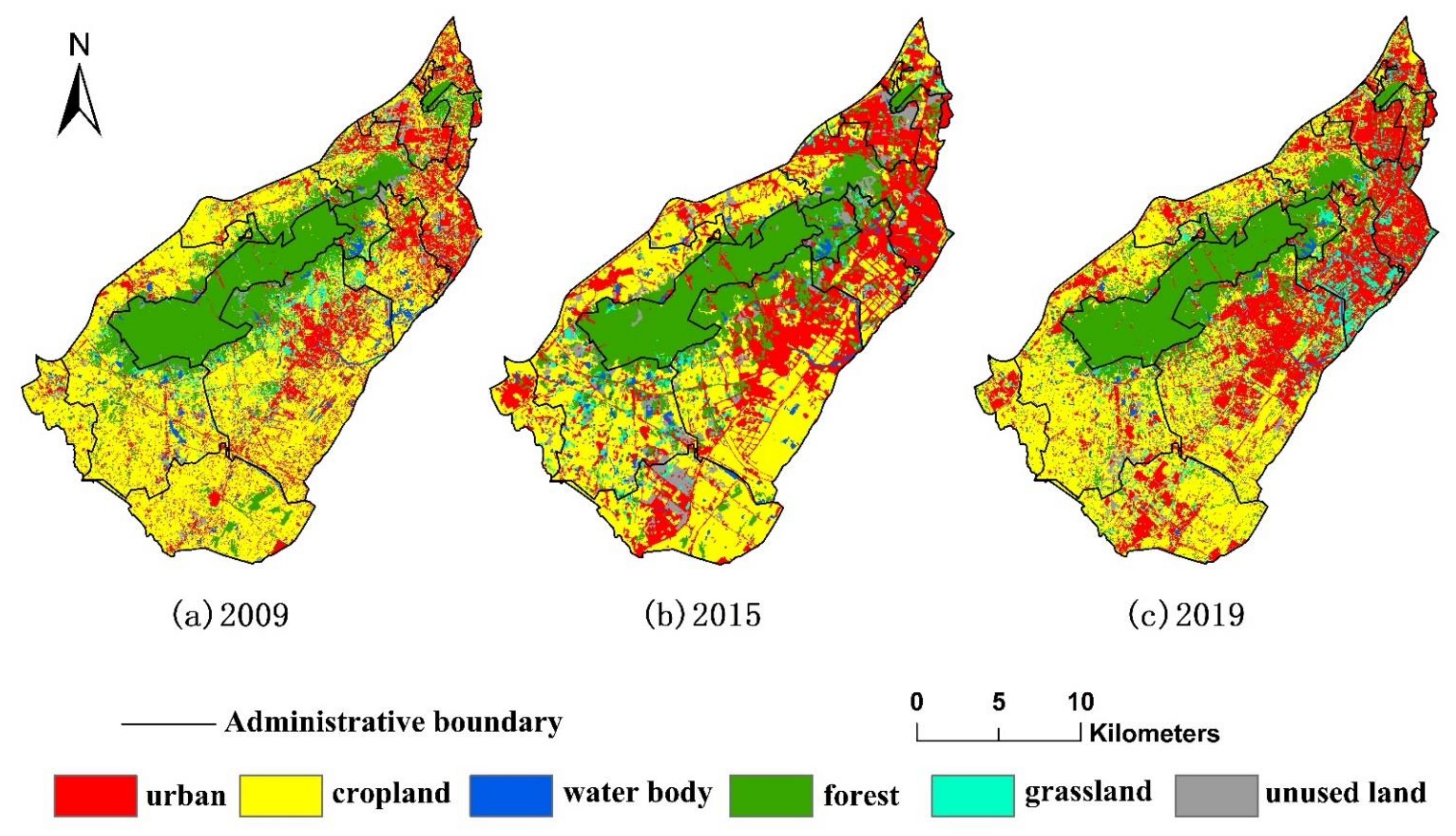
3.2. Spatial-Temporal Conversion Analysis of the Land Cover Types

Table 4. Transition matrix, LC area, and ACR from 2009 to 2019.

		Final	Urban	Cropland	Water Body	Forest	Grassland	Unused Land
	Initial
2009–2019 (km2) 2009–2015 (%)	urban		116.09 (39.86)	47.72 (42.23)	3.67 (54.50)	10.67 (49.95)	13.02 (34.95)	4.65 (48.82)
	cropland		74.67 (63.49)	223.11 (55.16)	3.67 (72.16)	33.75 (53.21)	30.91 (48.04)	13.29 (58.62)
	water body		6.01 (80.20)	7.12 (54.21)	8.16 (48.41)	1.70 (47.65)	1.31 (48.09)	0.78 (46.15)
	forest		13.79 (39.88)	27.39 (40.64)	0.83 (66.27)	148.87 (50.14)	7.60 (52.24)	3.58 (57.82)
	grassland		9.00 (63.33)	8.98 (32.96)	1.37 (35.77)	3.89 (45.76)	3.63 (49.59)	0.81 (40.74)
	unused land		15.40 (35.32)	15.40 (31.10)	0.65 (46.15)	6.00 (61.33)	3.88 (33.25)	2.30 (43.91)
Area/km2	2009		80.67	214.31	14.52	97.81	16.65	13.17
	2015		115.74	166.21	10.68	104.21	13.84	27.12
	2019		119.93	164.63	7.93	100.67	33.39	11.62
Annual change rate (%)	2009–2015		7.24	−3.74	−4.41	1.09	−2.82	17.64
	2015–2019		0.91	−0.24	−6.44	−0.85	35.31	−14.29

shows the results of the LC transition analysis. During the 10 years, the cropland accounted for the largest area. Forest ranked second in 2009 and shifted to third in 2015 due to the rapidly expanding urban land. The cropland decreased sharply, and the area of urban land and unused land increased from 2009 to 2015. The area of unused land decreased, and the area of urban green land (grassland) increased from 2015 to 2019.

Specifically, urban areas increased by 35.07 km² from 2009 to 2015 and only by 4.19 km² in the next four years, and the ACR decreased by 6.33%, indicating that the rate of urbanization had decreased. In 2009, urban areas were connected by roads, and the density of urban land was relatively low. Subsequently, separate urban areas spread and were combined into patches. In 2015, the density of urban land had increased substantially; especially, the streets along the Yangtze River had expanded (Figure 3).

The unused land increased by 13.95 km², of which 5.44 km² was converted to urban land from 2009 to 2015. The unused land decreased by 15.5 km², representing the largest reduction among all LC types due to the conversion to cropland and urban land from 2015 to 2019. Before and after the establishment of the JBNA in 2015, the unused land underwent significant changes. The ACR ranged from 17.64% to −14.29%, reflecting the process of urban construction from breaking ground to restoration during the 10 years.

From 2009 to 2015, the grassland area changed only slightly, and most areas were located around the Laoshan Forest Farm. Significant changes occurred from 2015 to 2019, with an increase of 19.55 km². The grassland area in the dense urban areas along the Yangtze River increased substantially. The cropland area decreased considerably by 48.10 km², with the largest reduction among all LC types from 2009 to 2015. Most of the area was converted to urban land (22.11%), and some areas were converted to forest and grassland. However, the cropland area remained stable since 2015. During the 10 years, water bodies and forest areas remained relatively stable. A slight reduction in forest land occurred around the Laoshan Forest Farm near towns and cultivated lands where the forest was significantly fragmented. A slight decrease in the water bodies occurred, and the area was mainly converted to cropland from 2009 to 2015 in the southern part of Dingshan St.

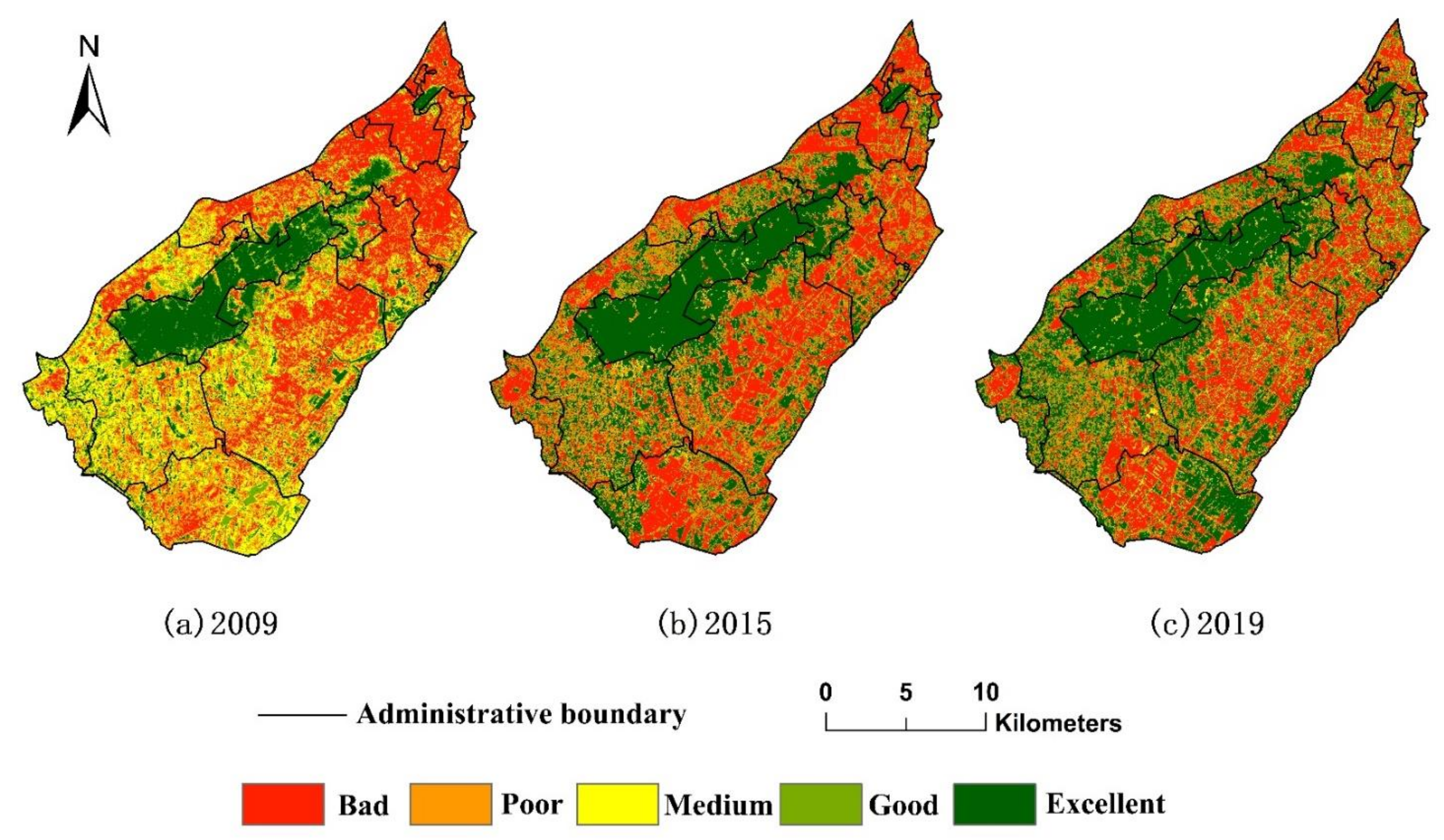
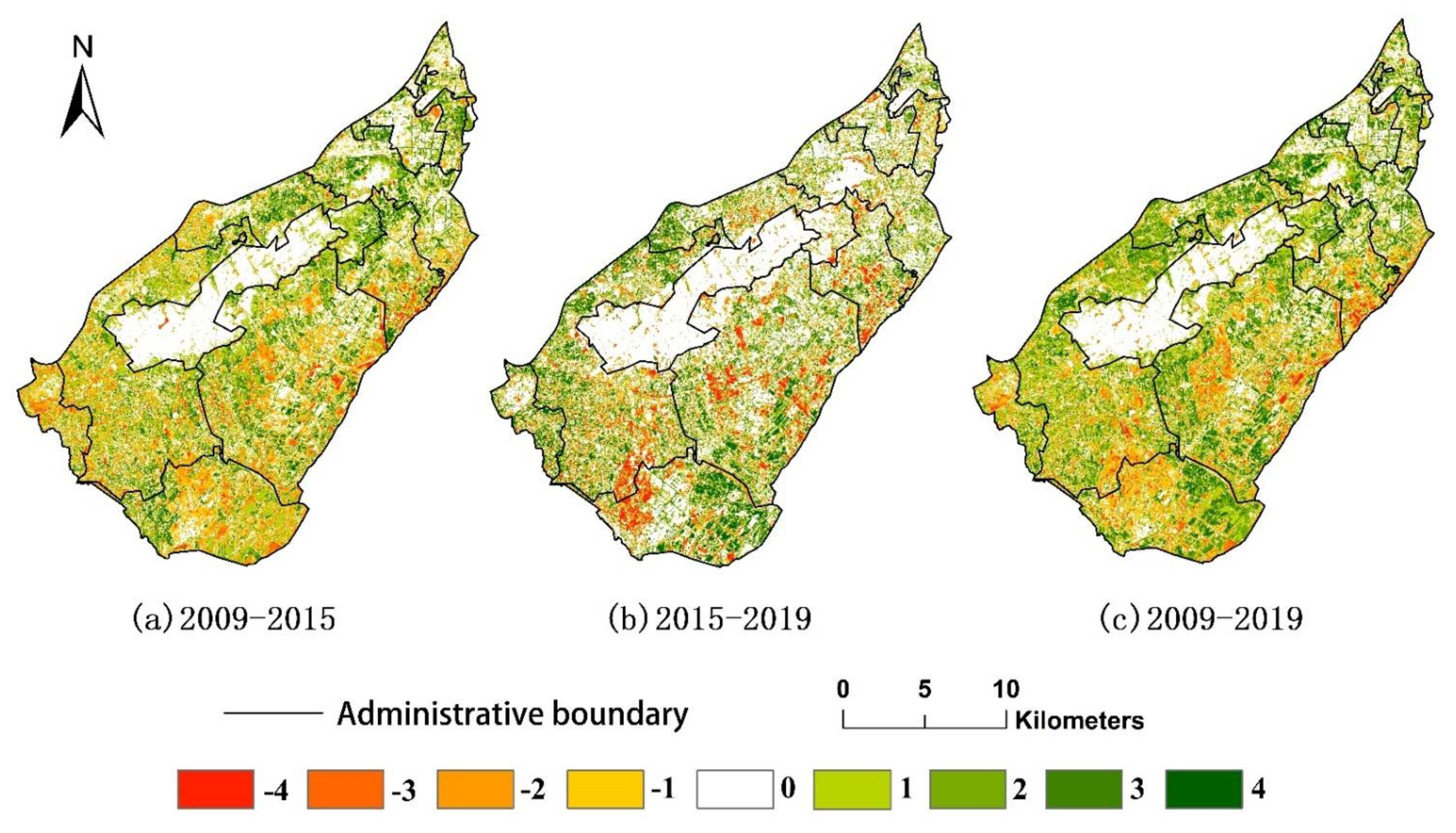
3.3. The Spatio-Temporal Transformation of Ecological Quality

Figure 4 illustrates the spatio-temporal patterns of the RSEI. The average RSEI values obtained from the Landsat images analyses of the study area were 0.583 in 2009, 0.559 in 2015, and 0.579 in 2019 (

Table 5. The results of the indicators of the RSEI and the average RSEI values.

Indicator	PC1			Mean
	2009	2015	2019	2009	2015	2019
NDVI	0.066	0.042	0.08	0.706	0.731	0.795
Wet	0.457	0.272	0.96	0.463	0.516	0.507
LST	−0.197	−0.126	−0.545	0.654	0.631	0.58
NDBSI	−0.193	−0.135	−0.728	0.431	0.474	0.631
Eigenvalues	0.267	0.358	0.322
Eigenvalue contribution (%)	66.4	61.02	56.37
RESI				0.583	0.559	0.579

). Overall, the ecological quality of the region decreased slightly and then increased slightly from 2009 to 2019.

The RSEI was divided into five levels at intervals of 0.2 (Xu, 2013) [28] (bad, poor, medium, good, and excellent) (Figure 4) to analyze the temporal and spatial changes in the ecological quality from 2009 to 2019 qualitatively. The area and proportion of the five RSEI levels in the three years are summarized in

Table 6. The area and proportion of the RSEI levels, representing the ecological quality.

RSEI Level	2009		2015		2019
	Area/km2	Proportion/%	Area/km2	Proportion/%	Area/km2	Proportion/%
Bad (0–0.2)	109.77	25.10	136.34	31.18	122.44	28.00
Poor (0.2–0.4)	111.14	25.42	91.53	20.93	61.33	14.03
Medium (0.4–0.6)	95.87	21.92	9.79	2.24	17.86	4.08
Good (0.6–0.8)	53.04	12.13	57.71	13.20	80.46	18.40
Excellent (0.8–1.0)	67.45	15.43	141.89	32.45	155.17	35.49

. The proportion of the excellent ecological quality class increased substantially from 15.43% to 35.49%, and the proportion of good ecological quality class increased slightly from 12.13% to 18.40%. The area of the medium ecological quality dropped sharply, and that of the poor ecological quality dropped slightly. The area of the bad ecological quality class increased and then decreased.

Figure 5 and

Table 7. The area and proportion of the changes in the ecological quality levels.

Change	Level Change	2009–2015		2015–2019		2019–2009
		Area/km2	Proportion/%	Area/km2	Proportion/%	Area/km2	Proportion/%
Deterioration	−4	3.50	27.91	13.61	20.59	3.83	24.62
	−3	10.94		21.53		10.48
	−2	36.43		12.34		32.82
	−1	71.18		42.53		60.51
Invariability	0	150.69	34.46	212.93	48.7	136.40	31.19
Amelioration	1	73.35	37.63	43.84	30.72	72.56	44.19
	2	45.09		35.21		62.77
	3	37.01		41.77		49.14
	4	9.07		13.5		14.22

show a downward trend in the area and proportion of the ecological quality levels from 2015 to 2019. The change area for the “Deterioration” category is smaller than the “Invariability” and “Amelioration” categories. Figure 5 indicates the following spatial changes in the ecological quality in the study area during the past 10 years.

From 2009 to 2015, most of the “Invariability” category occurred in the Laoshan Forest Farm and the existed construction area of the high-tech development zone and Taishan St. areas of ecological quality improvement were located in the northern streets. A deterioration of ecological quality primarily occurred along the Yangtze River, including along Dingshan St., Jiangpu St., and Qiaolin St., where areas of new urbanization and unused land were located. Areas of degeneration also occurred near Xingdian St., where mining areas caused ecological impacts, near Tangquan St. and Yongning St., where a township was developed, and at the border between Jiangpu St. and Laoshan Forest Farm, where forest fragmentation occurred.

From 2015 to 2019, the ecological quality of the densely constructed area along the Yangtze River improved in areas surrounding the built-up area. The ecological quality of the Laoshan–Qiaolin–Third Yangtze River Bridge ecological corridor (where Tangquan St. and Qiaolin St. border Jiangpu St.) improved.

Besides, due to the construction of forest infrastructure and tourism development, small areas (strip-like areas) of ecological quality deterioration occurred in the Laoshan Forest Farm from 2009 to 2019.

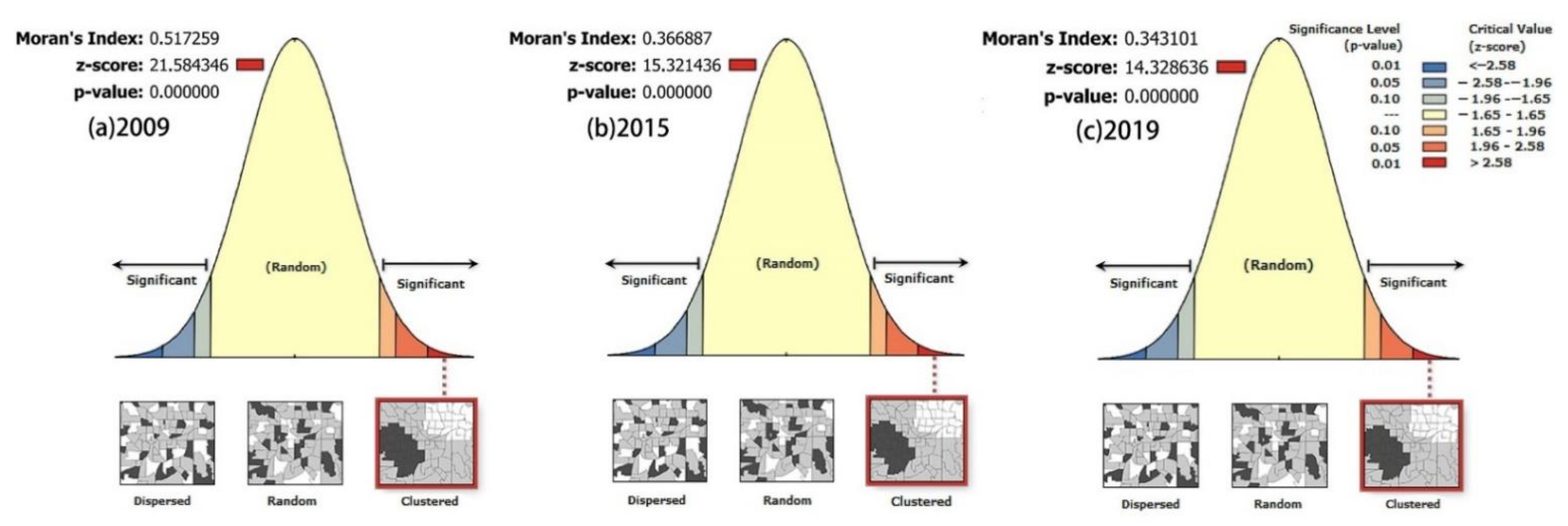
3.4. Spatial Auto-Correlation Analysis

Figure 6 shows the statistics of global Moran’s I value and the corresponding z-scores and $p$-values, at 0.517, 21.584, and 0 in 2009, 0.367, 15.3214, and 0 in 2015, and 0.343, 14.3286, and 0 in 2019, respectively, showing a decreasing trend in Moran’s I value. Moran’s I was highest in 2009, indicating that there was a strong positive correlation and certain internal connection between the ecological environment quality in the study area. The spatial distribution of ecological environment quality was clustered rather than random. The degree of auto-correlation became weaker since 2009 as the Moran’s I decreased, the spatial distribution became more dispersed.

Figure 7 shows the hot-spot and cold-spot analysis results of the RSEI. The red dots represent hot spots (high RSEI values), indicating the spatial clustering locations with high ecological quality. The blue dots represented cold spots (low RSEI values), indicating spatial clustering locations with low ecological quality.

In 2009, the hot spots with 99% confidence were mainly located in the core area of the Laoshan Forest Farm, and the 95% confidence hot spots were located at the periphery of the Laoshan Forest Farm and the Lvshuiwan Wetland Park along the Yangtze River. The cold spots with 99% confidence were mainly concentrated in highly industrialized areas, including the high-tech development zone, Taishan St., and Dingshan St. in the north. The cold spots with 95% confidence were mainly distributed in residential areas surrounding the industrial parks and areas with weaker exploitation intensity, as well as unused land around urban buildings.

In 2015, the distribution of the hot spots with 99% confidence remained almost unchanged, whereas the 95% confidence hot spots increased slightly and moved inside the Laoshan Forest Farm and west of Qiaolin St. A large number of cold spots moved southwest to Jiangpu St. and Qiaolin St.

In 2019, the hot spots with 95% confidence increased in the north of Laoshan Forest Farm and the intersection of Laoshan Forest Farm, Tangquan St., and Yongning St. There were also 95% confidence hot spots in the south of Xingdian St. and the east and west of Qiaolin St. The range of cold spots continued to expand compared with 2015. The increase in the 95% confidence cold spots was in agreement with the urban development and construction trajectory of Jiangpu St. and Qiaolin St., showing a radial spread.

A comparison of the distribution of the hot and cold spots with the LC cover distributions from 2009 to 2019 indicates that the distribution of the impervious layer, bare soil, and vegetation is consistent with the spatial aggregation and distribution of the cold and hot spots.

4. Discussion and Policy Implications

4.1. LC and Ecological Quality Changes Resulting from Traditional Urbanization (2009–2015) and NTU (2015–2019)

Our results demonstrated that the average value of ecological quality in the study area decreased from 0.583 in 2009 to 0.559 in 2015 and then rebounded to 0.579 in 2019. The results are in line with previous studies, which indicated that the average ecological condition in the Pukou district deteriorated from 2009 to 2015 [32,33]. Although the area ratio of the “Amelioration” category was higher than that of the “Deterioration” category in terms of ecological quality changes (Table 7), and the ecological quality of the area around Laoshan Forest Farm improved, the overall RSEI decreased by 3.79% from 2009 to 2015. We demonstrated that changes in urban land and bare land represented by the NDBSI had a substantial impact on ecological quality (Table 5) because LC change directly influences ecological service functions. Therefore, improvements in ecological quality were limited during the traditional and extensive urbanization period in the study area (2009 to 2015) due to the expansion of construction land and bare land. This observation is in agree with Hang’s findings in Nanjing from 2000 to 2018 [32].

This study revealed similarities in the spatial pattern between LC change and RSEI change, which was confirmed in the spatial auto-correlation analysis. Many of the cold spots (99% and 95% confidence) moved to Dingshan St., Jiangpu St., and Qiaolin St. from 2009 to 2015 due to diverse urban construction and development projects, for example, the policy evolution and major catalysts (Youth Olympics) promoted the development of streets along the Yangtze River. Many urban construction projects, including real estate construction, transportation, and urban infrastructure, led to a change in the distribution of the low clusters of RSEI (cold spots).

Traditional rapid urbanization focuses only on the population size and the scale of cities, with a limited focus on development quality and ecological environments [60]. Our findings regarding the LC and ecological quality changes from 2009 to 2015 confirmed this. During this period, the JBNA was undergoing a traditional urbanization process that resulted in vegetation degradation, a sharp decline in cultivated land, and a decline in ecological functions. Besides, according to data from the Nanjing Statistical Yearbook (

Table 8. Data from the Nanjing Statistical Yearbook from 2009–2019.

Year	Pukou District				Nanjing City
	Per Capita Disposable Income of Urban Residents (Yuan)	Rural Economic Conditions (10,000 People)			Per Capita Green Area (m2)	Green Coverage Rate in Built-Up Area (%)	Green Coverage Area (hm2)
		Total Registered Population	Agriculture, Forestry, Animal Husbandry, and Fishery Employees	Number of Industrial Employees
2009	23,542	54.87	2.61	4.07
2010					13.69	44.38	84,848
2015	43,687	64.28	2.06	4.2	15.1	44.47	96,874
2019	59,807	76.49	1.71	2.79	15.7	45.16	101,327

), urban sprawl, population growth, and rapid economic growth led to an increasing demand for working and living spaces. Hence, it is urgent to improve the urban ecological environment in this area through NTU.

To implement the NTU process, the Nanjing government and Nanjing Jiangbei New Area Management Committee issued corresponding plans, including the “Urban and Rural Construction Outline for the 13th Five-Year Plan of Nanjing” and the “Master Plan of Nanjing Jiangbei New Area (2014–2030)”. Under the guidance of these plans, NTU considers the integrity of economic and social forces, as well as the improvement of natural amenities and ecosystem diversity. The establishment and protection of national parks, watershed restoration, moderate conversion of cropland to forest or grassland, and expansion of urban green space will contribute to the improvement of environmental quality [61].

The Master Plan (nanjing.gov.cn accessed on 15 March 2021) includes 52 ecological red line divisions in the JBNA, with a total area of 543 km², accounting for about 22.2% of the total JBNA area. We found that the protection regimes were implemented strictly inside the ecological red line of the Laoshan Forest Farm, leading to sustained high ecological quality from 2009 to 2019. The increase in forest land resulted from ecological improvements. Small forest land reduction occurred primarily in locations of significant forest fragmentation, such as the boundaries between the Laoshan Forest Farm and towns and cultivated land.

Our study also found that the rate of urbanization slowed down from 2009 to 2015. Increases in urban areas and unused land occurred mostly due to cropland conversion. Intense urbanization and ecological construction have led to a substantial reduction in cropland. However, the state must ensure a sufficient cropland area to maintain national food security [62]. The “Master Plan for Land Use in Pukou District, Nanjing (2006–2020)” requires the protection of cropland to ensure the requirements of quantity, quality, and ecology (referred to as a trinity). Thus, the cropland area has remained stable since 2015 due to the cropland red line and cropland protection policies. In contrast, a slight increase in the urban area occurred due to conversion from unused land from 2015 to 2019. Thus, we confirmed that the increase and decrease in the amount of unused land were mostly driven by construction needs in line with the plan to ensure adequate urban development and improve livability.

In addition, the grassland in urban areas has increased sharply since 2015. Since the integration of urban construction space and green space were considered in the JBNA development, an increase in the grassland area was vital for urban ecological restoration and livability and occurred in response to the call for “ecological use, ecological security, and green development” of land [63]. Besides, grassland areas can be developed more quickly and economically than urban woodland to improve urban green space rapidly.

According to the Master Plan, the JBNA green space system in the study area includes the core development zone, the ecological protection zone along the Yangtze River, and the Laoshan–Qiaolin–Third Yangtze River Bridge ecological corridor. The RSEI results showed that the ecological quality of the green space system was maintained and improved (see Figure 4 and Figure 5 or Table 6 and Table 7). The green space in Nanjing changed from being disorderly to orderly, and its layout changed from plaque fragmentation to a system network [64]. The per capita green area (m²), the green coverage rate in the built-up area (%), and the green coverage area (hm²) of Nanjing all increased from 2009 to 2019 (Table 8). We believe that these observations are attributable to the environmentally friendly development strategies or the plans enforced by different governmental agencies that restored urban ecology. Thus, the NTU process in the research area achieved good initial results.

4.2. Uncertainties and Future Work

Although the differences between different sensors were minimized as much as possible, some deviations were observed in the LC due to the different capabilities of the sensors for detecting details. Although multi-scale segmentation is a powerful technique for dealing with high-resolution imagery, some segmented objects did not match the geometries of the target objects [21], which may have reduced the classification accuracy. Besides, due to the lack of scientific spatial planning in the study area before the establishment of the JBNA, the spatial layout is scattered and fragmented, increasing the difficulty of classification, especially in the urban–rural fringe areas. Thus, we used visual interpretation after site surveys to improve the classifications.

The RSEI model also has some limitations for assessing regional ecological quality. The ecological quality of cropland is affected by seasonal influences and changes to bare land after harvesting. Therefore, it is critical to use remote sensing images with similar acquisition dates [5]. Since deep learning methods have been increasingly used in remote sensing image processing [65], we will consider using deep learning for the LC classification and RSEI modeling in the future to improve the analysis accuracy.

Despite these limitations, our study provided more details, and the results are more applicable than those of previous similar studies. We created high-accuracy land cover conversion results as bases. The RSEI model can describe the ecological equality in a quantitative way and provide direct insights regarding future landscape planning and management. For the first time in this special pioneering region, we observed the specific changes before and after the implementation of the NTU process because we elaborately tuned a crucial study time span by selecting suitable remotely sensed multi-source images. Our study results also confirmed the initial effect of the NTU process on the improvement of the regional ecological environment. It indeed balanced the contradiction between the growing urban economic and demographic development demand and the livability of the study area. Thus, the study results can inform relevant municipal, district, and street departments of the direction for the future urban ecological planning and the further improvement of inhabitants’ living environment. Particularly, when carrying out vigorous rural construction under a socialist framework and implementing a rural revitalization strategy, the cropland red line and rural revitalization policies should be strictly abided by to not only promote rural economy rapid development [66], but also pay priority to the development of tourism resources and ecological construction and conservation.

5. Conclusions

In this study, we used object-oriented classification and an LC transformation matrix to analyze LC changes resulting from urban expansion. The RSEI model was used to determine ecological quality changes in the JBNA from 2009 to 2019. We subsequently examined the effects of LC changes on the ecological environment and elucidated the spatio-temporal relationship between the LC changes and RSEI during periods of traditional urbanization and NTU. It was found that the NTU that prioritizes ecological development used in 2015–2019 was a greener approach than the traditional urbanization process in 2009–2015. This finding demonstrates the effectiveness of the NTU strategy that balances environmental protection and economic development.

We found that the urban area increased throughout the entire study period, but the rate of increase slowed down in the latter stage, indicating that the urbanization process had become more focused on quality and balanced development. Existing urban areas saw intensive development, urban green spaces were utilized, unused land was efficiently allocated, urban functions were considered, and the living and working environment was improved. Moreover, the results indicated that the initial traditional urbanization limited improvements in the ecological environment. The environmental quality improved after scientific spatial planning, green industrial transformation, and construction to improve livability. Increases in the green space in the JBNA to a large extent alleviated the reduction of ecological quality caused by urbanization. Thus, we found that the NTU contributed to maintaining or improving the quality of the urban ecological environments, providing an example for urbanization in other regions.

References

1. Lambin, E.; Rounsevell, M.; Geist, H. Are agricultural land-use models able to predict changes in land-use intensity? Agric. Ecosyst. Environ. 2000, 82, 321–331. [Google Scholar] [CrossRef]
2. Cai, Y.-B.; Li, H.-M.; Ye, X.-Y.; Zhang, H. Analyzing Three-Decadal Patterns of Land Use/Land Cover Change and Regional Ecosystem Services at the Landscape Level: Case Study of Two Coastal Metropolitan Regions, Eastern China. Sustainability 2016, 8, 773. [Google Scholar] [CrossRef] [Green Version]
3. He, X.; Liang, J.; Zeng, G.; Yuan, Y.; Li, X. The Effects of Interaction between Climate Change and Land-Use/Cover Change on Biodiversity-Related Ecosystem Services. Glob. Chall. 2019, 3, 1800095. [Google Scholar] [CrossRef] [PubMed] [Green Version]
4. Lin, M.; Lin, T.; Sun, C.; Jones, L.; Sui, J.; Zhao, Y.; Liu, J.; Xing, L.; Ye, H.; Zhang, G.; et al. Using the Eco-Erosion Index to assess regional ecological stress due to urbanization—A case study in the Yangtze River Delta urban agglomeration. Ecol. Indic. 2019, 111, 106028. [Google Scholar] [CrossRef]
5. Xu, H.; Wang, M.; Shi, T.; Guan, H.; Fang, C.; Lin, Z. Prediction of ecological effects of potential population and impervious surface increases using a remote sensing based ecological index (RSEI). Ecol. Indic. 2018, 93, 730–740. [Google Scholar] [CrossRef]
6. Chen, M.; Liu, W.; Lu, D.; Chen, H.; Ye, C. Progress of China’s new-type urbanization construction since 2014: A preliminary assessment. Cities 2018, 78, 180–193. [Google Scholar] [CrossRef]
7. Li, H.; Song, W. Evolution of rural settlements in the Tongzhou District of Beijing under the new-type urbanization policies. Habitat Int. 2020, 101, 102198. [Google Scholar] [CrossRef]
8. Yao, X.; Kou, D.; Shao, S.; Li, X.; Wang, W.; Zhang, C. Can urbanization process and carbon emission abatement be harmonious? New evidence from China. Environ. Impact Assess. Rev. 2018, 71, 70–83. [Google Scholar] [CrossRef]
9. Deng, S. Exploring the relationship between new-type urbanization and sustainable urban land use: Evidence from prefecture-level cities in China. Sustain. Comput. Inform. Syst. 2020, 30, 100446. [Google Scholar] [CrossRef]
10. Zhao, Z.; Bai, Y.; Wang, G.; Chen, J.; Yu, J.; Liu, W. Land eco-efficiency for new-type urbanization in the Beijing-Tianjin-Hebei Region. Technol. Forecast. Soc. Chang. 2018, 137, 19–26. [Google Scholar] [CrossRef]
11. Zhao, Y.; Wang, S.; Zhou, C. Understanding the relation between urbanization and the eco-environment in China’s Yangtze River Delta using an improved EKC model and coupling analysis. Sci. Total. Environ. 2016, 571, 862–875. [Google Scholar] [CrossRef]
12. Shen, W.; Mao, X.; He, J.; Dong, J.; Huang, C.; Li, M. Understanding Current and Future Fragmentation Dynamics of Urban Forest Cover in the Nanjing Laoshan Region of Jiangsu, China. Remote. Sens. 2020, 12, 155. [Google Scholar] [CrossRef] [Green Version]
13. Lü, Y.; Ma, Z.; Zhang, L.; Fu, B.; Gao, G. Redlines for the greening of China. Environ. Sci. Policy 2013, 33, 346–353. [Google Scholar] [CrossRef]
14. Yang, J.; Li, Y.; Hay, I.; Huang, X. Decoding national new area development in China: Toward new land development and politics. Cities 2019, 87, 114–120. [Google Scholar] [CrossRef]
15. Kabisch, N.; Selsam, P.; Kirsten, T.; Lausch, A.; Bumberger, J. A multi-sensor and multi-temporal remote sensing approach to detect land cover change dynamics in heterogeneous urban landscapes. Ecol. Indic. 2018, 99, 273–282. [Google Scholar] [CrossRef]
16. Zhu, X.; Liu, D. Improving forest aboveground biomass estimation using seasonal Landsat NDVI time-series. ISPRS J. Photogramm. Remote. Sens. 2015, 102, 222–231. [Google Scholar] [CrossRef]
17. Duro, D.; Franklin, S.; Dubé, M.G. A comparison of pixel-based and object-based image analysis with selected machine learning algorithms for the classification of agricultural landscapes using SPOT-5 HRG imagery. Remote. Sens. Environ. 2012, 118, 259–272. [Google Scholar] [CrossRef]
18. Batista, M.H.; Haertel, V. On the classification of remote sensing high spatial resolution image data. Int. J. Remote. Sens. 2010, 31, 5533–5548. [Google Scholar] [CrossRef]
19. Hu, Q.; Wu, W.; Xia, T.; Yu, Q.; Yang, P.; Li, Z.; Song, Q. Exploring the Use of Google Earth Imagery and Object-Based Methods in Land Use/Cover Mapping. Remote. Sens. 2013, 5, 6026–6042. [Google Scholar] [CrossRef] [Green Version]
20. Rizvi, I.A.; Mohan, B.K. Improving the accuracy of object based supervised image classification using cloud basis function neural network for high resolution satellite images. Image Process. 2010, 4, 342–353. [Google Scholar]
21. Rizvi, I.A.; Mohan, B.K. Object-Based Image Analysis of High-Resolution Satellite Images Using Modified Cloud Basis Function Neural Network and Probabilistic Relaxation Labeling Process. IEEE Trans. Geosci. Remote. Sens. 2011, 49, 4815–4820. [Google Scholar] [CrossRef]
22. Blaschke, T. A framework for change detection based on image objects. Göttinger Geogr. Abh. 2005, 113, 1–9. [Google Scholar]
23. Blaschke, T. Object based image analysis for remote sensing. ISPRS J. Photogramm. Remote. Sens. 2010, 65, 2–16. [Google Scholar] [CrossRef] [Green Version]
24. Chen, Y.; Jiang, H.; Li, C.; Jia, X.; Ghamisi, P. Deep Feature Extraction and Classification of Hyperspectral Images Based on Convolutional Neural Networks. IEEE Trans. Geosci. Remote. Sens. 2016, 54, 6232–6251. [Google Scholar] [CrossRef] [Green Version]
25. Zhao, W.; Du, S.; Emery, W.J. Object-Based Convolutional Neural Network for High-Resolution Imagery Classification. IEEE J. Sel. Top. Appl. Earth Obs. Remote. Sens. 2017, 10, 3386–3396. [Google Scholar] [CrossRef]
26. LeCun, Y.; Bengio, Y.; Hinton, G. Deep learning. Nature 2015, 521, 436–444. [Google Scholar] [CrossRef]
27. Ma, L.; Liu, Y.; Zhang, X.; Ye, Y.; Yin, G.; Johnson, B.A. Deep learning in remote sensing applications: A meta-analysis and review. ISPRS J. Photogramm. Remote. Sens. 2019, 152, 166–177. [Google Scholar] [CrossRef]
28. Maggiori, E.; Tarabalka, Y.; Charpiat, G.; Alliez, P. Convolutional Neural Networks for Large-Scale Remote-Sensing Image Classification. IEEE Trans. Geosci. Remote. Sens. 2016, 55, 645–657. [Google Scholar] [CrossRef] [Green Version]
29. Willis, K.S. Remote sensing change detection for ecological monitoring in United States protected areas. Biol. Conserv. 2015, 182, 233–242. [Google Scholar] [CrossRef]
30. Zhou, D.; Zhao, S.; Liu, S.; Zhang, L.; Zhu, C. Surface urban heat island in China’s 32 major cities: Spatial patterns and drivers. Remote. Sens. Environ. 2014, 152, 51–61. [Google Scholar] [CrossRef]
31. Ivits, E.; Cherlet, M.; Mehl, W.; Sommer, S. Estimating the ecological status and change of riparian zones in Andalusia assessed by multi-temporal AVHHR datasets. Ecol. Indic. 2009, 9, 422–431. [Google Scholar] [CrossRef]
32. Murray, N.J.; Keith, D.A.; Bland, L.M.; Ferrari, R.; Lyons, M.B.; Lucas, R.; Pettorelli, N.; Nicholson, E. The role of satellite remote sensing in structured ecosystem risk assessments. Sci. Total Environ. 2018, 619-620, 249–257. [Google Scholar] [CrossRef] [PubMed] [Green Version]
33. Hu, X.; Xu, H. A new remote sensing index for assessing the spatial heterogeneity in urban ecological quality: A case from Fuzhou City, China. Ecol. Indic. 2018, 89, 11–21. [Google Scholar] [CrossRef]
34. Xu, H. A remote sensing urban ecological index and its application. Acta Ecol. Sin. 2013, 24, 7853–7862. [Google Scholar]
35. Yuan, F.; Bauer, M.E. Comparison of impervious surface area and normalized difference vegetation index as indicators of surface urban heat island effects in Landsat imagery. Remote. Sens. Environ. 2006, 106, 375–386. [Google Scholar] [CrossRef]
36. Gupta, K.; Kumar, P.; Pathan, S.; Sharma, K. Urban Neighborhood Green Index—A measure of green spaces in urban areas. Landsc. Urban Plan. 2012, 105, 325–335. [Google Scholar] [CrossRef]
37. Hang, X.; Li, Y.; Luo, X.; Xu, M.; Han, X. Assessing the Ecological Quality of Nanjing during Its Urbanization Process by Using Satellite, Meteorological, and Socioeconomic Data. J. Meteorol. Res. 2020, 34, 280–293. [Google Scholar] [CrossRef]
38. Yue, H.; Liu, Y.; Li, Y.; Lu, Y. Eco-Environmental Quality Assessment in China’s 35 Major Cities Based on Remote Sensing Ecological Index. IEEE Access 2019, 7, 51295–51311. [Google Scholar] [CrossRef]
39. Shan, W.; Jin, X.; Ren, J.; Wang, Y.; Xu, Z.; Fan, Y.; Gu, Z.; Hong, C.; Lin, J.; Zhou, Y. Ecological environment quality assessment based on remote sensing data for land consolidation. J. Clean. Prod. 2019, 239, 118126. [Google Scholar] [CrossRef]
40. Ariken, M.; Zhang, F.; Liu, K.; Fang, C.; Kung, H.-T. Coupling coordination analysis of urbanization and eco-environment in Yanqi Basin based on multi-source remote sensing data. Ecol. Indic. 2020, 114, 106331. [Google Scholar] [CrossRef]
41. European Space Agency. Available online: https://www.esa.int/ (accessed on 15 March 2021).
42. Gong, P.; Chen, B.; Li, X.; Liu, H.; Wang, J.; Bai, Y.; Chen, J.; Chen, X.; Fang, L.; Feng, S.; et al. Mapping essential urban land use categories in China (EULUC-China): Preliminary results for 2018. Sci. Bull. 2019, 65, 182–187. [Google Scholar] [CrossRef] [Green Version]
43. Drǎguţ, L.; Tiede, D.; Levick, S. ESP: A tool to estimate scale parameter for multiresolution image segmentation of remotely sensed data. Int. J. Geogr. Inf. Sci. 2010, 24, 859–871. [Google Scholar] [CrossRef]
44. Drăguţ, L.; Csillik, O.; Eisank, C.; Tiede, D. Automated parameterisation for multi-scale image segmentation on multiple layers. ISPRS J. Photogramm. Remote. Sens. 2013, 88, 119–127. [Google Scholar] [CrossRef] [PubMed] [Green Version]
45. Abdullah, A.Y.M.; Masrur, A.; Adnan, M.S.G.; Al Baky, A.; Hassan, Q.K.; Dewan, A. Spatio-temporal Patterns of Land Use/Land Cover Change in the Heterogeneous Coastal Region of Bangladesh between 1990 and 2017. Remote. Sens. 2019, 11, 790. [Google Scholar] [CrossRef] [Green Version]
46. Rimal, B.; Zhang, L.; Keshtkar, H.; Haack, B.N.; Rijal, S.; Zhang, P. Land Use/Land Cover Dynamics and Modeling of Urban Land Expansion by the Integration of Cellular Automata and Markov Chain. ISPRS Int. J. Geo-Inf. 2018, 7, 154. [Google Scholar] [CrossRef] [Green Version]
47. Hishe, S.; Bewket, W.; Nyssen, J.; Lyimo, J. Analysing past land use land cover change and CA-Markov-based future modelling in the Middle Suluh Valley, Northern Ethiopia. Geocarto Int. 2019, 35, 225–255. [Google Scholar] [CrossRef]
48. Crist, E.P. A TM Tasseled Cap equivalent transformation for reflectance factor data. Remote. Sens. Environ. 1985, 17, 301–306. [Google Scholar] [CrossRef]
49. Yarbrough, L.D.; Easson, G.; Kuszmaul, J.S. Using at-sensor radiance and reflectance tasseled cap transforms applied to change detection for the ASTER sensor. IEEE 2005, 141–145. [Google Scholar] [CrossRef]
50. Zhang, X.; Schaaf, C.B.; Friedl, M.A.; Strahler, A.H.; Gao, F.; Hodges, J.C.F. MODIS tasseled cap transformation and its utility. Int. Geosci. Remote Sens. Symp. 2002, 2, 1063–1065. [Google Scholar] [CrossRef]
51. United States Geological Survey (USGS). Landsat 8 Data Users Hand Book; Geological Survey, Department of the Interior: Reston, VA, USA, 2016.
52. Liu, G.; Zhang, Q.; Li, G.; Doronzo, D.M. Response of land cover types to land surface temperature derived from Landsat-5 TM in Nanjing Metropolitan Region, China. Environ. Earth Sci. 2016, 75, 1386. [Google Scholar] [CrossRef]
53. Sobrino, J.A.; Jiménez-Muñoz, J.C.; Paolini, L. Land surface temperature retrieval from LANDSAT TM 5. Remote. Sens. Environ. 2004, 90, 434–440. [Google Scholar] [CrossRef]
54. Rikimaru, A.; Roy, P.S.; Miyatake, S. Tropical forest cover density mapping. Trop. Ecol. 2002, 43, 39–47. [Google Scholar]
55. Xu, H. A new index for delineating built-up land features in satellite imagery. Int. J. Remote. Sens. 2008, 29, 4269–4276. [Google Scholar] [CrossRef]
56. Getis, A.; Ord, J.K. The analysis of spatial association by use of distance statistics. Geogr. Anal. 2010, 24, 189–206. [Google Scholar] [CrossRef]
57. Anselin, L. Local Indicators of Spatial Association-LISA. Geogr. Anal. 2010, 27, 93–115. [Google Scholar] [CrossRef]
58. Unwin, D.J. GIS, spatial analysis and spatial statistics. Prog. Hum. Geogr. 1996, 20, 540–551. [Google Scholar] [CrossRef]
59. Ord, J.K.; Getis, A. Local Spatial Autocorrelation Statistics: Distributional Issues and an Application. Geogr. Anal. 1995, 27, 286–306. [Google Scholar] [CrossRef]
60. Yu, B. Ecological effects of new-type urbanization in China. Renew. Sustain. Energy Rev. 2020, 135, 110239. [Google Scholar] [CrossRef]
61. Xu, F.; Wang, Z.; Chi, G.; Zhang, Z. The impacts of population and agglomeration development on land use intensity: New evidence behind urbanization in China. Land Use Policy 2020, 95, 104639. [Google Scholar] [CrossRef]
62. Lai, Z.; Chen, M.; Liu, T. Changes in and prospects for cultivated land use since the reform and opening up in China. Land Use Policy 2020, 97, 104781. [Google Scholar] [CrossRef]
63. Liu, Y.; Li, J.T.; Yang, Y. Strategic adjustment of land use policy under the economic transformation. Land Use Policy 2018, 74, 5–14. [Google Scholar] [CrossRef]
64. Shen, S. Dynamic simulation of urban green space evolution based on Camarkov model-a case study of Hexi new town of Nanjing city, China. Appl. Ecol. Environ. Res. 2019, 17. [Google Scholar] [CrossRef]
65. Khelifi, L.; Mignotte, M. Deep Learning for Change Detection in Remote Sensing Images: Comprehensive Review and Meta-Analysis. IEEE Access 2020, 8, 126385–126400. [Google Scholar] [CrossRef]
66. Wan, J.; Su, Y.; Zan, H.; Zhao, Y.; Zhang, L.-Q.; Zhang, S.; Dong, X.; Deng, W. Land Functions, Rural Space Governance, and Farmers’ Environmental Perceptions: A Case Study from the Huanjiang Karst Mountain Area, China. Land 2020, 9, 134. [Google Scholar] [CrossRef]
Figure 1. Schematic map of the study area.
Sustainability 13 11979 g001
Figure 2. The administrative divisions of the study area.
Sustainability 13 11979 g002
Figure 3. The LC maps in 2009, 2015, and 2019.
Sustainability 13 11979 g003
Figure 4. The maps of the RSEI levels in 2009, 2015, and 2019.
Sustainability 13 11979 g004
Figure 5. The change in the RSEI levels from 2009 to 2015, 2015 to 2019, and 2009 to 2019.
Sustainability 13 11979 g005
Figure 6. Spatial auto-correlation analysis result of the RSEI in 2009, 2015, and 2019.
Sustainability 13 11979 g006
Figure 7. Results of the RSEI hot-spot and cold-spot analysis during 2009 to 2019.
Sustainability 13 11979 g007