Optimization of PEMFC Model Parameters Using Meta-Heuristics

Abstract

The present study introduces an economical–functional design for a polymer electrolyte membrane fuel cell system. To do so, after introducing the optimization problem and solving the problem based on the presented equations in the fuel cell, a cost model is presented. The final design is employed for minimizing the construction cost of a 50 kW fuel cell stack, along with the costs of accessories regarding the current density, stoichiometric coefficient of the hydrogen and air, and pressure of the system as well as the temperature of the system as optimization parameters. The functional–economic model is developed for the studied system in which all components of the system are modeled economically as well as electrochemically–mechanically. The objective function is solved by a newly improved metaheuristic technique, called converged collective animal behavior (CCAB) optimizer. The final results of the method are compared with the standard CAB optimizer and genetic algorithm as a popular technique. The results show that the best optimal cost with $0.1061 \$/\mathrm{kWh}$ is achieved by the CCAB. Finally, a sensitivity analysis is provided for analyzing the consistency of the method.

1. Introduction

To directly convert chemical energy into electricity without combustion, an electrochemical device called a fuel cell is used. Thanks to this characteristic, it has higher electrical performance toward thermal motors, which are restricted by the performance of the Carnot cycle. The by-product of reacting in a fuel cell can be heat, water, carbon dioxide, and hydrocarbons, according to the type of consumed fuel. Gas diffusion layers, gaskets, flow-field plates, collector plates, catalyst layers, and Larminie and Dicks are the main components of this device [1]. The system supplies the requested energy, while the fuel and the oxidizer are existing. To provide the desired current and voltage, they can make series or parallel connections.

The benefits of fuel cells include cleanliness, connection to micro-turbines, silent operation, no moving elements, and lower greenhouse effects [2,3,4]. Among different types of fuel cells, the polymer electrolyte membrane fuel cell (PEMFC), because of its several advantages, is considered the popular one. Some of these advantages are lower weight, lower temperatures of operation, higher density of operation, and capability for decreasing price. The PEMFC is a widely used fuel cell among different power levels that was initially modeled to be used in a spacecraft at NASA. The main fuel of this device is hydrogen. The operating temperature of a PEMFC is imitated to the range between 70 °C and 80 °C. To provide faster electrochemical reactions, expensive catalysts, such as platinum, were utilized in this type of fuel cell [5,6]. Some prominent advantages of PEMFCs is their higher startup speed, higher density of power, and lower temperature of operation. Electrodes, end plates, washers, dipoles, and ion exchange membranes are the most important components of the polymer membrane fuel cell. In the last years, optimization of this system was noticed by researchers, and various economic and functional designs have been presented [7,8].

The modeling of the fuel cell stacks is performed to obtain two significant purposes. The first one is to estimate the efficiency of the fuel cell by polarization curve analysis, and the next purpose is to investigate the fuel cell stack while the cell operates; this helps to propose an optimum design for it. The primary mathematical PEMFC design was presented in the year 1992, and the achievements indicated good structure with the experimental data [9].

Solsona et al. [8] introduced a control-oriented model to analyze the low-temperature PEMFC. The results were then verified based on the empirical data from $Nafio{n}^{\circledR }$ PEMFC, including a humidifier. The comparison of the proposed model with the empirical data confirmed the method efficiency for the analysis of the fuel cell.

Hirano et al. [10] analyzed a PEMFC performance based on numerical analysis. To do the analysis, a model was proposed to indicate the correlations of fuel cell performance, features of the material, and gas diffusion layers. The results were analyzed by performing it on the PEMFC numerical model.

Taleb et al. [11] presented a fractional order–based design of a PEMFC stack. The primary objective was to model the PEMFC system based on a fractional calculation to obtain accurate and compact results. The final results confirmed that the obtained values by the proposed method have proper similarity to the laboratory test bench.

Kumar et al. [12] presented a different design for PEMFCs. The method was then analyzed based on ARX and ARMAX validation to verify the method modality. To obtain the proper load current, the study utilized PID and PI controllers. The MATLAB platform was used for the design simulations.

As it is clear, various classic methods exist for this system identification. However, although the introduced methods’ application for the identification of the PEMFC is so profitable, they have a big shortcoming. Due to the consideration of all physical concepts of PEMFC by the classic methods, such as power, thermodynamics, momentum’s conservation, the complexity of the model is increased.

Furthermore, to develop the precision of the model and to obtain a favorable accuracy, compared with the empirical data, it needs to consider the best amounts for the model parameters. Recently, different types of approaches were presented for this purpose. The use of meta-heuristic algorithms, due to their ability for faster and simpler solving of nonlinear models, are exponentially increasing [13,14,15,16]. Some examples of these methods are the dragonfly algorithm [17], deer hunting optimizer [18_ENREF_20], multi-verse optimizer [19_ENREF_18], improved invasive weed optimization algorithm [20_ENREF_19], and chaotic grasshopper optimizer [21].

Duan et al. [13] proposed an optimal design for the PEM fuel cell stack by the satin bowerbird optimization algorithm (SBOA). The SBOA algorithm is employed to optimize the procedure efficiency analysis. A comparison of the results with several various approaches was performed to indicate the method’s performance. The achievements were also verified by the experimental data to show the algorithm’s performance.

Carton et al. [22] presented a 3D electrochemical design for an OPCF. The presented model was then compared with a double channel simulation and empirical data that showed a promising match with the empirical data. Simulation results showed that the flow plates in OPCF develop the fluid distribution in this device by 54% performance at 0.7 V.

Cao et al. [15] utilized an improved optimization technique for modeling, designing, and simulating the PEMFC systems with an optimal solution. The optimization method was defined by the seagull optimizer, and the purpose was to use that tool for the best identification of parameters of the PEMFC stack. The model was then assessed by two empirical PEMFC models and was put in comparison with several meta-heuristics to indicate the efficiency of the algorithm.

Yu et al. [23] introduced another method for the PEMFC parameter estimation to develop the model performance. The study proposed the optimization of ENN for this purpose. The optimization was based on the blending of two new optimizers: the World Cup optimizer (WCO) and fluid search optimizer (FSO). The achievements showed better accuracy of the proposed model than the PEM fuel cell design parameters.

Fathy et al. [24] suggested a combined differential evolution and vortex search optimizer for optimal PEMFC parameter estimation. After the design and simulation, the analysis was applied to four experimental benchmarks to show the efficiency of the method. The achievements verified the excellence of the presented approach, compared with the other methods.

Generally, optimizers have proper results for the PEM fuel cell model, which is thanks to the proper capability of them to avoid the local minima, compared to the classic approaches [25,26,27]. A new optimal design for a PEM fuel cell-based system is presented in this paper. The model parameters are then optimized by a newly developed collective animal behavior optimizer (CAB). The results are then validated by empirical data to show the method’s precision.

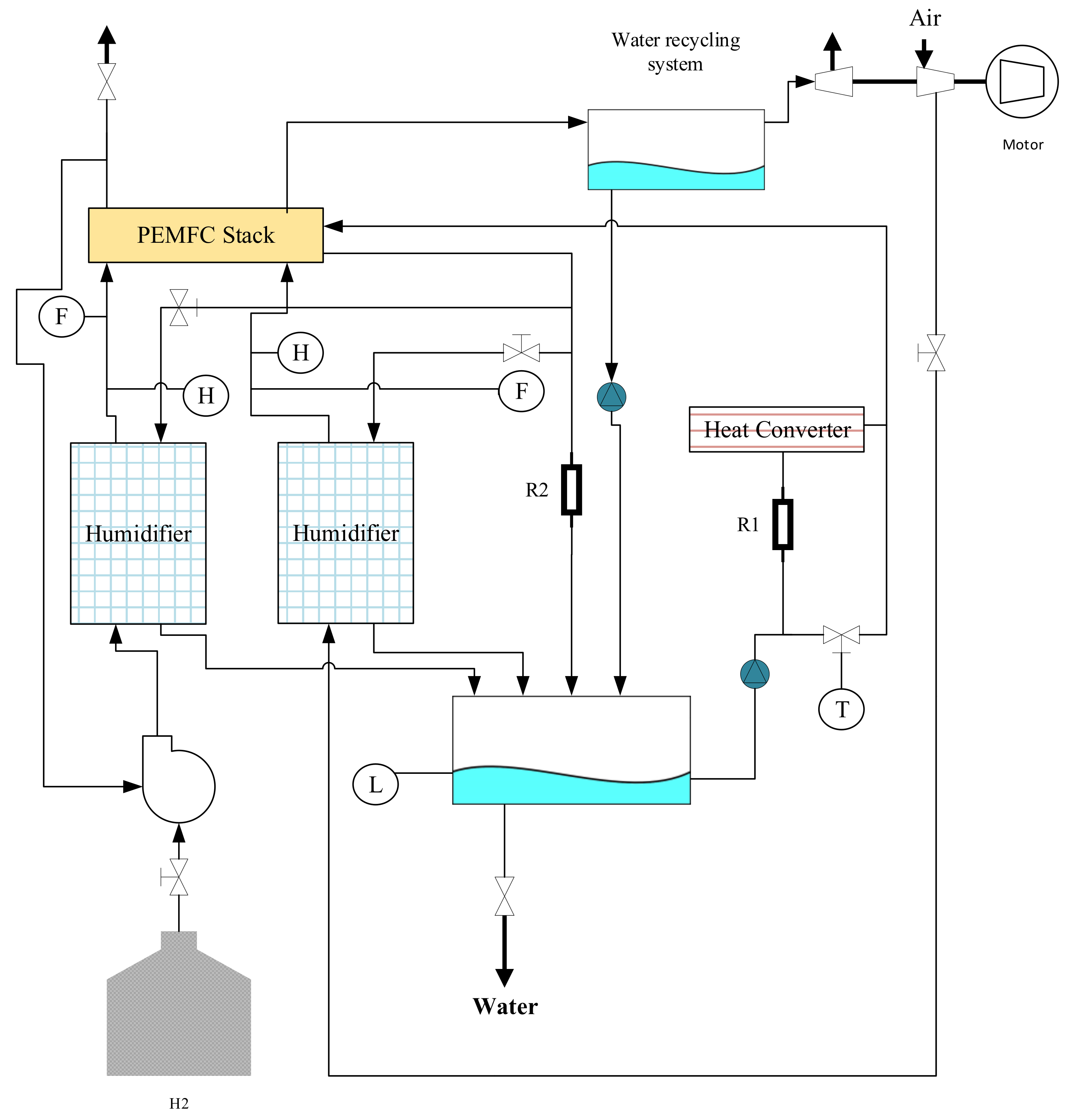
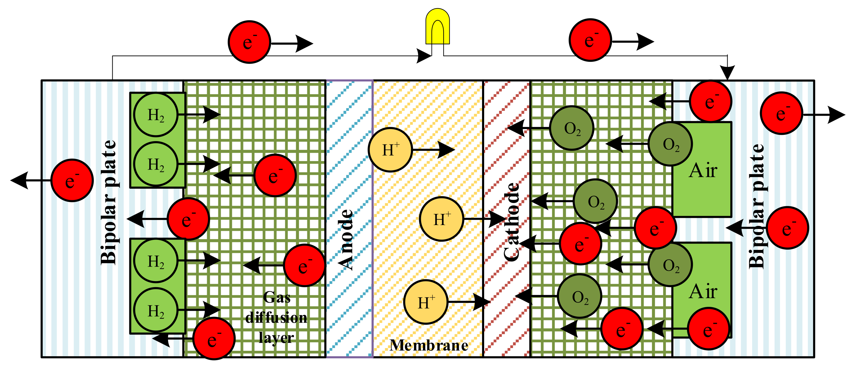
2. The Model of the Studied System

The overall structure of the analyzed model is depicted in Figure 1. The model considered in this study has a $50 \mathrm{kW}$ fuel cell stack. These types of fuel cells are widely used in vehicles, power plants, military and space equipment, and heat and power cogeneration systems. The air entering the fuel cell passes through the compressor and then enters the compressor after the pressure rises. In this system, humidifiers, pumps, and electrical control devices are considered system peripheral parts. The main purpose of the optimal modeling in the fuel cell stack is to obtain optimal values for the system pressure parameters, its input hydrogen and air, its operational temperature, and its density of current flow to provide the minimum feasible cost.

After modeling the system, the next step is to solve the problem, formulate the objective function, and model it concerning the parameters defined. In the following, the objective of the system is given in detail.

Modeling of the Fuel Cell

The system objective function under study is the minimization of the overall cost, including the cost of investment ($C_0$) and the operating cost ($C_t$) by considering the discount rate ($R_d$) as follows:

$$C=C_0+{\displaystyle \sum }_{t=1}^n\frac{C_t}{{\left(1+R_d\right)}^t}$$

(1)

The investment cost of the fuel cell stack includes the storage tank ($C_{st}$), stack ($C_{stack}$), auxiliary costs ($C_{aux}$), and fuel costs ($C_{fuel}$), i.e.,

$$C_0=C_{st}+C_{stack}+C_{fuel}+C_{aux}$$

(2)

The fuel cell stack of a PEMFC includes different components, such as electrodes, ion exchange membranes, screws, bipolar surfaces, gaskets, and end plates, and other joints. The utilized catalyst in the stack is platinum that has its share in the cost of making the system. The overall cost ($\$/{\mathrm{m}}^2$) is calculated from the following equation [28]:

$$C_{stack}=\left(C_{montage}+\frac{c_{mem}+c_e+c_{bp}+c_{pt}+c_{ex}}{10\times V_t\times i}\right)$$

(3)

where $c_{mem}$ describes the cost of the membrane ($\$/{\mathrm{m}}^2$), $c_e$ is the cost of the electrode ($\$/{\mathrm{m}}^2$), $c_{bp}$ determines the cost of the bipolar plates ($\$/{\mathrm{m}}^2$), $c_{ex}$ describes the cost of auxiliaries, such as washers and end plates ($\$/{\mathrm{m}}^2$), $C_{montage}$ determines the cost of the stack montage ($\$/{\mathrm{m}}^2$), $V_t$ determines the fuel cell voltage ($v$), $i$ represents the cell density, and $c_{pt}$ is the cost of the platinum ($\$/{\mathrm{m}}^2$) that is achieved based on the following equation:

$$c_{pt}=C_{ptg}\times M_{pt}$$

(4)

where$C_{ptg}$ describes the cost of each kilogram of platinum ($\$/\mathrm{kg}$) and $M_{pt}$ stands for the amount of catalyst used ($\mathrm{kg}/{\mathrm{m}}^2$).

In the above relation, the cost of electrodes, the cost of the bipolar plates, and the lateral costs of transport are independent of the current density, while the current density depends on the rate of the catalysis and membrane performance. To calculate the fuel cost, all the input costs to the system are consumed, so the fuel cost is calculated from the underlying relationship.

$$C_{fuel}=c_{H2}\times P_{stack}\times {\eta }_{stack}^{-1}\times H_{2}T{V}^{-1}$$

(5)

where $c_{H2}$ describes the cost of each kilogram of $H_2$, $P_{stack}$ represents the fuel cell power, $\eta$ determines the stack performance, and $H_{2}TV$ is the thermal value of hydrogen ($\mathrm{kJ}/\mathrm{kg}$). Figure 2 shows the general structure of a PEMFC [29].

The cost of an ancillary system, which is known as the equilibrium cost, is a fraction of the fuel storage and the stack costs, and includes the costs of the compressor, humidifier, electrical control equipment, and other auxiliary equipment in the system. It is formulated as follows [29]:

$$C_{aux}=0.51\times \left(C_{st}+C_{stack}\right)\times {\eta }_{FC}$$

(6)

The following equation indicates the unit operating cost, and since these costs are continuously generated by the operation of the power generation system over 90 months, they must be adjusted accordingly. In this study, the manufacturing time of the stack is not considered; only its costs are taken into account, and the time taken into account is also the time of the cell’s operation [29].

$$C_t={\left(1+R_i\right)}^{t-1}{C}_0+3600\times {\left(1-R_{fi}\right)}^{t-1}{C}_{H_2}\times \frac{t_0\times c_f\times {\lambda }_{H_2}}{6480\times V_t\times i}$$

(7)

where $R_i$ describes the inflation ratio, $R_{fi}$ represents the fuel inflation ratio, ${\lambda }_{H_2}$ is the hydrogen stoichiometric coefficient, and $t_0$ is the functional lifetime of the fuel cell.

All of the simulation is returned for 90 months, which is the fuel cell’s operating lifetime. Both the investment cost and the operational cost are a function of the stack efficiency. The system efficiency is achieved by dividing the net output power by the net input power [30].

$${\eta }_{FC}=-\frac{V_t\times {\mu }_s\times \left(P_{stack}-P_{aux}\right)}{1.25\times P_{stack}}$$

(8)

where $P_{stack}$ describes the fuel cell’s stack power ($w$), $P_{aux}$ represents the power of the peripheral devices ($w$), and ${\mu }_s$ determines the inverse stoichiometric coefficient.

Since in the studied system, the compressor and other peripherals use the power of this system, to obtain the system’s net outputted power, the power of the peripherals should be decreased by the achieved power from the fuel cell [31]. The constant 1.25 in the denominator is also an experimental coefficient that is intended for the fuel cell stack systems to operate the system with considering the peripherals, so the stack efficiency is a function of the cell voltage, stack power, stoichiometric fuel rate, and power of other accessories.

There are three main voltage losses in the fuel cell: activation voltage loss, Ohmic voltage loss, and over-potential saturation voltage loss. So, based on [32,33], the output fuel cell voltage is achieved by the following equation:

$$V_t=N_{nc}\times \left(E_N-E_O-E_{ops}-E_{op}\right)$$

(9)

where $E_N$ describes the Nernst relation and defines the cell voltage reversibility, $N_{nc}$ determines the connected cells’ number, $E_O$ stands for the Ohmic voltage loss, $E_{ops}$ refers to the overpotential saturation, and $E_{op}$ describes the activation overpotential per cell. The Nernst equation for the PEM fuel cell is obtained as follows [34]:

$$E_N=1.23-8.5\times {10}^{-4}\left(T_{PEM}-298.15\right)+4.31\times {10}^{-5}\times T_{PEM}\times \left[ln\left(P_{H_2}\right)+0.5\times ln\left(P_{O_2}\right)\right]$$

(10)

where,

$$P_{O_2}=R_{hc}\times P_{H_{2}O}\left[\frac{1}{\frac{R_{hc}\times P_{H_{2}O}}{P_c}\times e^{\frac{1.635I_{FC}/A}{T^{1.334}{I}_{FC}}}}-1\right]$$

(11)

$$P_{H_2}=\frac{R_{ha}\times P_{H_{2}O}}{2}\left[\frac{1}{\frac{R_{ha}\times P_{H_{2}O}}{P_a}\times e^{\frac{1.635I_{FC}/A}{T^{1.334}{I}_{FC}}}}-1\right]$$

(12)

where $A$ determines the active area of the membrane,$I_{FC}$ represents the operational current of the fuel cell, $P_a$ and $P_c$ describe the partial pressures as an inlet for positive and negative electrodes, respectively, and $R_{ha}$ and $R_{hc}$ stand for the electrodes’ relative humidity. $P_{H_{2}O}$ is the saturation vapor pressure in the PEMFC and can be calculated as the following given equation [35]:

$$lo{g}_{10}\left(P_{H_{2}O}\right)=0.0295\times \left(T_{FC}-273.15\right)-2.18-9.18\times {10}^{-5}{T}_c^2+1.4\times {10}^{-7}{T}_c^3$$

(13)

In the operating changes, the reference temperature is considered 25 °C.

The formulation of the Ohmic voltage loss can be defined as follows:

$$E_O=I_{FC}\times \left(R_m+R_c\right)$$

(14)

where,

$$R_m={\rho }_m\times l\times S^{-1}$$

(15)

$${\rho }_m=\frac{181.6\left[1+0.062{\left(\frac{T_{FC}}{303}\right)}^2\times {\left(\frac{I_{FC}}{S}\right)}^{2.5}+0.03\left(\frac{I_{FC}}{S}\right)\right]}{\left[\lambda -0.063-3\left(\frac{I_{FC}}{S}\right)\right]\times e^{\frac{T_{FC}-303}{T_{FC}}}}$$

(16)

The overpotential activation voltage drop is calculated as given below:

$$E_{op}=-\left[{\gamma }_1+{\gamma }_2\times T_{FC}+{\gamma }_3\times T_{FC}\times \ln \left(C_{O_2}\right)+{\gamma }_4\times T_{FC}\times \ln \left(I_{FC}\right)\right]$$

(17)

where,

$${\gamma }_2=4.3\times {10}^{-5}\ln \left(C_{H_2}\right)+2.1\times {10}^{-4}\ln \left(A\right)+2.9\times {10}^{-3}$$

(18)

where $C_{O_2}$ and $C_{H_2}$ illustrate the saturation of $O_2$ and $H_2$ in the cathode’s catalytic interface ($\mathrm{mol}/{\mathrm{cm}}^3$), which are achieved as follows:

$$C_{O_2}=\frac{P_{O_2}}{5.1\times {10}^6}\times e^{\frac{498}{T_{FC}}}$$

(19)

$$C_{H_2}=\frac{P_{H_2}}{1.1\times {10}^6}\times e^{\frac{-77}{T_{FC}}}$$

(20)

The over-potential saturation ($E_{ops}$) is formulated by the following equation [15]:

$$E_{ops}=-\beta \times ln\left(J_{max}-\frac{J}{J_{max}}\right)$$

(21)

where $I$ is the membrane thickness; $S$ refers to the membrane surface (${\mathrm{cm}}^2$); I_FC is the PEMFC operating current; $T_{FC}$ defines the operating temperature of the cell (°C); ${\beta }_i$ describes the experimental coefficients; $\lambda$ determines the controlling parameter; $\beta$ defines a parametric coefficient; ${\rho }_m$ is the membrane resistivity; $J$ determines the standard current density and J_max is the highest current density; $P_H$, $P_{O_2}$, and $P_{H_{2}O}$ are the partial pressure of the H₂, O₂ and H₂O, respectively; P_a describes the inlet pressure for the anode and P_c for the cathode; $R_{hc}$ represents the vapor relative humidity at the cathode and $R_{ha}$ the anode; C_H2 is the hydrogen saturation and C_O2 is the oxygen saturation (mol/cm³); and R_m and R_c are the membrane and connection resistances, respectively.

Table 1. The optimal results of parameters based on [15].

Parameter	Value	Parameter	Value
${\beta }_1$	−1.03	$\beta$	0.01
${\beta }_2\times {10}^{-3}$	3.48	$R_c\times {10}^{-4}$	1.63
${\beta }_3\times {10}^{-5}$	7.79	$\mathsf{\lambda }$	15.04
${\beta }_4\times {10}^{-5}$	−9.48

illustrates the optimal value of some undefined parameters based on [15].

On the other hand, to calculate the stack efficiency, in addition to being specific to the stack’s power, the auxiliary (accessory) power must also be calculated. It should be noted that the extra power supply for the 50 kW power production is estimated to be 5.2 kW based on [36].

$$P_{com}=C_P\times \frac{T_e}{{\eta }_m{\eta }_{mt}}\left({\left(\frac{P_{sys}}{P_{in}}\right)}^{0.26}-1\right)\times \dot{m}$$

(22)

where$T_e$ is the input air temperature (°C), $P_{in}$ and $P_{sys}$ are the input and the system pressures ($atm$), and the following holds:

$$\dot{m}=35.7\times {10}^{-7}\times {\lambda }_{air}\times i\times A\times N$$

(23)

Another investment term is the fuel storage cost that is calculated by the following equation:

$$C_{st}=\frac{C_{s}1}{A\times F\times V_t}$$

(24)

where $F$ determines the Faraday constant, $A$ is the cell area (${\mathrm{m}}^2$), $t$ describes the fuel cell performance time ($9 \mathrm{month}/\mathrm{year}$), and $C_s$ describes the hydrogen’s storage cost per kg that is determined based on the hydrogen amount stored as defined below:

$$C_s=\left\{\begin{array}{c}5.244 \$/\mathrm{kg} for 27,000 \mathrm{kg}\\ 1.752 \$/\mathrm{kg} for 276,000 \mathrm{kg}\\ 1.044 \$/\mathrm{kg} for 27,600,000 \mathrm{kg}\end{array}\right.$$

(25)

As aforementioned, the independent variables of the model are the stack operating temperature, system pressure, air stoichiometric coefficient, and hydrogen as the system inputs as well as the current density. The operating temperature of the system shall be such that it protects both the high temperature of the water and water vapor and does not cause the membrane to break. Therefore, its high level is considered to be $90 °\mathrm{C}$ and its low level is considered to be $60 °\mathrm{C}$. The stoichiometric coefficient of air and hydrogen is considered the ratio of each of the inlet gases to its theoretical value, so the minimum value of these values is set to 1. Since these values are not high, the upper limit is assumed to be 3. The system pressure cannot be lower than the atmospheric pressure, as the compressor is not capable of compressive pressure; therefore, the low pressure is 0.12 MPa and its upper limit is considered to be 0.48 bar [36]. The high and low current density limits are also equal to 1 and 0, respectively.

By the aforementioned equations, the objective function can be defined as given below:

$$\min C=C_0+{\displaystyle \sum }_{t=1}^n\frac{C_t}{{\left(1+R_d\right)}^t}$$

(26)

Such that the following holds:

$$\begin{gathered} 1\le {\lambda }_{air}\le 3 \\ 1\le {\lambda }_{H_2}\le 3 \\ 0.13\le P_{sys}\le 0.50 \\ 0\le i\le 1 \\ 60\le T\le 90 \end{gathered}$$

(27)

Converged Collective Animal Behavior Algorithm.

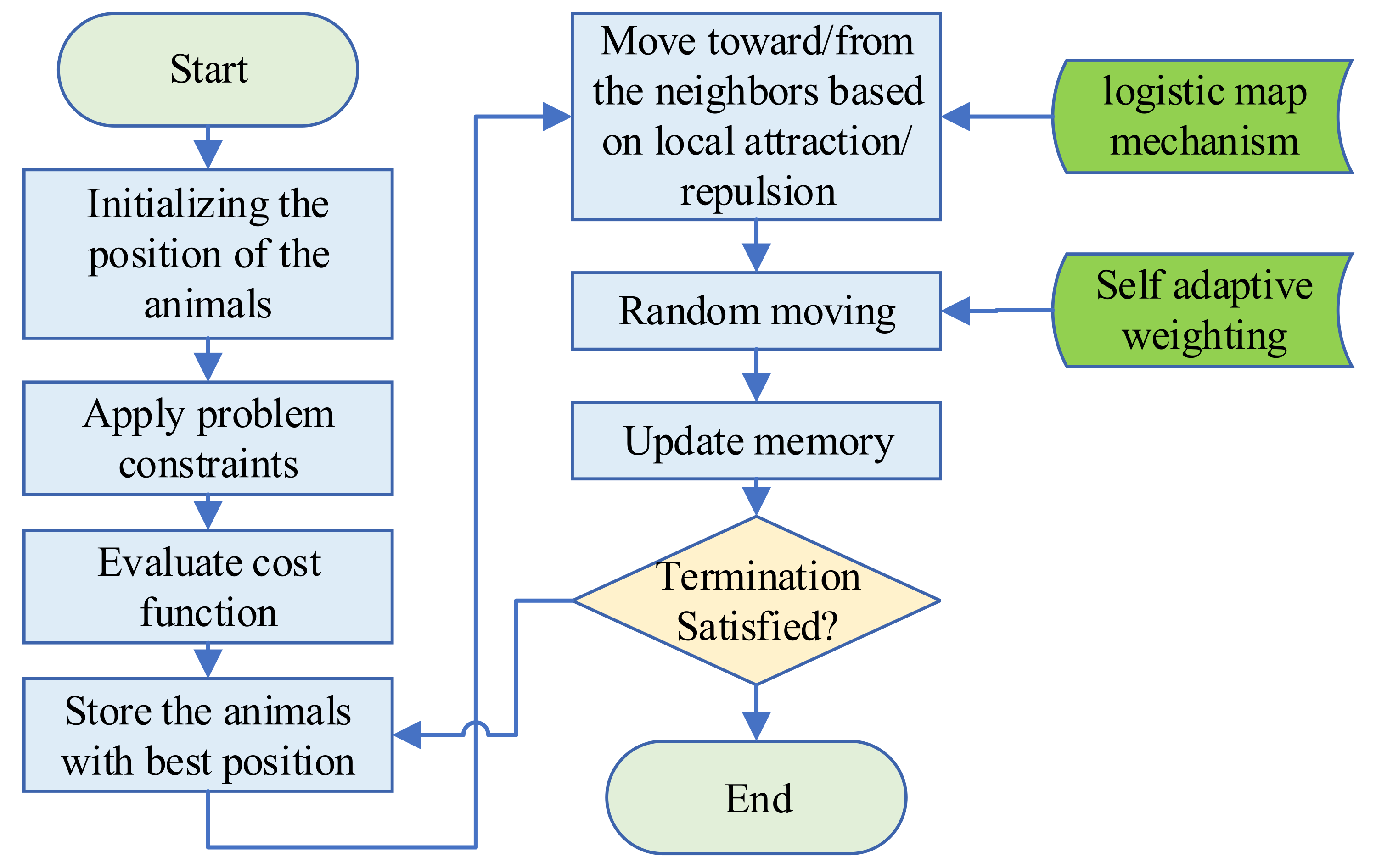
2.1. Collective Animal Behavior Algorithm

Meta-heuristic algorithms are based on stochastic searching the solution, and although only a few numbers were shown for converging to the best solution, the simple structure of them, high maneuverability, and above all their higher quickness made them popular optimization tools in the last years [23]. Recently, different models of meta-heuristics were introduced, which all have their strengths and weaknesses. Considering these characteristics and improving them based on different theories can make them stronger from their typical version with more profits. Meta-heuristic algorithms are inspired by different phenomena, from nature [26,37,38] to human social behaviors [25,39,40,41,42,43].

Cuevas et al. [44] proposed a new approach in 2019, which was an inspiration for collective animal behavior (CAB). The CAB algorithm was modeled based on a collection of different operations that simulate the association of social animal behaviors. Here, the problem solution is defined by the animal position that is placed in the solution space. The value of cost is also determined by animal dominance through the group. An advantage of this optimizer is that it considers a two-part memory for storing the optimal solutions based on previous experiences. One part is the memory that keeps the optimal location of the animal per iteration ($Mg$), and the next one stores the optimal historical locations over the optimization ($Mh$). A detailed description of the CAB algorithm is explained in the following.

The optimizer begins with some locations of the animal. The location of each animal, p contains a D–D vector with parameter values to be optimized. The CAB optimizer contains several identical random distributed amounts between the predetermined upper and minimum bounds such that the following holds:

$$\begin{gathered} p_{i,j}=p_j^L+\sigma \times \left[p_j^H-p_j^L\right] \\ j=1,2\cdots D; i=1,2\cdots N_a \end{gathered}$$

(28)

where $p_{i,j}$ determines the j^th parameter of the i^th animal,$\sigma$ represents a random integer by a mean value equal to 0 and value of variance of 1, j refers to the individual, and i the parameter indices.

After generating the new population, they are sorted and stored in the memories $Mg$ and $Mh$ following their cost function. During the operation of the swarm, the first B constituents (i.e., $\left[p_1,p_2\cdots p_B\right]$) of the new position for animals are obtained based on the historical memory M_h plus a slight randomly perturbation surrounding them, i.e.,

$$\begin{gathered} p_l=v+m_h^l \\ l\in \left[1,2\cdots B\right] \end{gathered}$$

(29)

where $m_h^l$ represents the l^th number of the M_h and v describes a randomly small length vector.

The algorithm uses a randomly local absorption by the individuals to improve the exploitation. This is performed by applying for an identical random number between 0 and 1. In this mechanism, if r_m has an amount higher than a determined threshold (T), it can be attracted to the nearest M_g in the solution space in the present iteration, and if the r_m has a value less than the threshold, a definite position for the animal can be attracted by the best nearest historical location (M_h):

$$p_i=\left\{\begin{array}{c}{x}_i\pm r_m\times \left(m_h^{\mathrm{closest}}-x_i\right) \mathrm{with\; probability} T\\ x_i\pm r_m\times \left(m_g^{\mathrm{closest}}-x_i\right) \mathrm{with\; probability} \left(1-T\right)\end{array}\right.$$

(30)

where $r_m$ describes a random value, and $m_h^{\mathrm{closest}}$ and $m_g^{\mathrm{closest}}$ determine the closest elements of M_g and M_h to x_i.

Afterward, for improving the random moving of the animals with probability $P_i$, the following model is considered:

$$\begin{gathered} p_i=\left\{\begin{array}{c}r \mathrm{with\; probability} Pr\\ x_i \mathrm{with\; probability} \left(1-Pr\right)\end{array}\right. \\ i=\left[B+1, B+2\cdots N_a\right] \end{gathered}$$

(31)

where r determines a random value for animal position initializing again randomly.

The animals with more communication have better value with the minimum distance, which depends on how the animals’ swarm behaves. So, during connecting the animals, the most dominant of them stay and the others are eliminated. The updating steps for historical memory are performed as follows:

Consider $M_U$ the total memory, i.e., $M_U=M_g+M_h$ Compare the i^th component of the memory M_U ($M_U^i$) with the rest elements of memory ($\left[m_U^1,m_U^2\cdots m_U^{2B-1}\right]$); if the distance <$\delta$, the animal with the better cost value remains and the other is eliminated.

The elements of M_U from phase 2 achieve the B optimum amount to build the new M_h.

The distance amount $\delta$ is formulated as shown below:

$$\delta =0.1\times D^{-1}\times {\displaystyle \prod }_{j=1}^D\left(p_j^{\mathrm{high}}-p_j^{\mathrm{low}}\right)$$

(32)

where $p_j^{\mathrm{high}}$ and $p_j^{\mathrm{low}}$ describe the pre-defined higher and minimum bound of the $j^{th}$ the variable in a D-dimensional space, respectively.

Converged CAB Algorithm

Among the different advantages of the CAB algorithm, it shows that sometimes, its solution gives premature convergence. Here, two important modifications are performed to resolve that shortcoming. The first modification is performed based on a self-adjustable weighting to handle the tendency speed to the optimal solution. To update the animals’ position in this way, a controlled random value is implemented on the swarm exploration and the “repulsive effect” terms. To make a proper balance between exploration and exploitation, initial iterations search with a high searching limit, and the final ones are explored by a local search. This mechanism was applied to the random movement term as shown below:

$$p_{i, \mathrm{new}}=\left\{\begin{array}{c}{p}_i+\gamma \times S\left(p_i\right)\otimes F_i, \mathrm{rand}>0.5\\ p_i-\gamma \times S\left(p_i\right)\otimes F_i, \mathrm{rand}\le 0.5\end{array}\right.$$

(33)

where,

$$\gamma =\left\{\begin{array}{c}{\left(\frac{f\left(p_{\mathrm{best}}\right)}{f\left(p_{\mathrm{worst}}\right)}\right)}^2, if f\left(p_{\mathrm{worst}}\right)\ne 0\\ 1 , if f\left(p_{\mathrm{worst}}\right)=0\end{array}\right.$$

(34)

where $f\left(p_{\mathrm{worst}}\right)$, and $f\left(p_{\mathrm{best}}\right)$ refer to the worst and the best solutions’ cost values, respectively, for the random moving.

Based on the mentioned structure, the weight value for the random moving is increased incrementally to reduce the best and the worst solutions’ differences.

The next mechanism that is employed here is the chaos approach, which is applied to resolve the local optimization problem. Based on the chaos mechanism, the optimal solution is sometimes likely to be stuck in the local optima, which makes a misleading solution for the other animals in the swarm, and, in following the local optimal solution, consequently, results in premature convergence.

To find a solution for this issue, the random values in the algorithm are turned into pseudo-random values by the chaos mechanism. This theory has sequences and ergodic random features that are very useful to develop the premature convergence of the algorithm [45,46]. In the proposed algorithm, the logistic map, as a widely used mechanism in chaos theory, is used. By algorithm development, the equations below are updated as follows:

$${\sigma }_{i+1}^{\mathrm{new}}={\sigma }_i^{\mathrm{new}}+{\rho }_i\times {\sigma }_i^{\mathrm{new}}$$

(35)

$$v_{i+1}^{\mathrm{new}}=v_i^{\mathrm{new}}+{\rho }_i\times v_i^{\mathrm{new}}$$

(36)

$$r_{i+1}^{\mathrm{new}}=r_i^{\mathrm{new}}+{\rho }_i\times r_i^{\mathrm{new}}$$

(37)

where,

$${\rho }_{i+1}=4{\rho }_i\left(1-{\rho }_i\right)$$

(38)

where ${\rho }_i$ describes the amount for the $i^{th}$ chaotic iteration, and the primary amount ${\rho }_1\in \left[0,1\right]$ is a random amount. Figure 3 shows the workflow of the suggested CCAB algorithm.

2.2. Algorithm Confirmation

To validate the proposed CCAB algorithm efficiency, some unimodal and multimodal test functions were utilized. The achievements of applying the suggested CCAB optimizer were put in comparison with several various meta-heuristic optimizers, the World Cup optimizer (WCO) [25], emperor penguin optimization (EPO) [47], gravitational search algorithm (GSA) [48], and typical CAB algorithm [44], to declare its high efficiency. The general information about the test functions for verification is given in

Table 2. The typical information of the test functions used for the confirmation.

Model	Function	Formulation	Optimum
Unimodal	Rotated High Conditioned Elliptic	$F_1(x)=f_1\left(M\left(x-o_1\right)\right)+F_1^{*}$	100
	Rotated Bent Cigar	$F_2(x)=f_2\left(M\left(x-o_2\right)\right)+F_2^{\ast }$	200
	Rotated Discuss	$F_3(x)=f_3\left(M\left(x-o_3\right)\right)+F_3^{\ast }$	300
Multimodal	Shifted and rotated Rosenbrock	$F_4(x)=f_4\left(M\left(\frac{2.048\left(x-o_4\right)}{100}\right)+1\right)+F_4^{\ast }$	400
	Shifted and rotated Ackley	$F_5(x)=f_5\left(M\left(x-o_5\right)\right)+F_8^{*}$	500

.

The population size for all the optimizers is set to be 120, and the stopping criteria are defined by the highest value of the evaluated functions. The dimension of the functions is equal to 30. The optimum effectiveness is obtained by runs of more than 45 as stated in

Table 3. Comparative achievements of the optimizers.

		GSA [48]	EPO [47]	WCO [25]	CAB [44]	CCAB
$F_1$	Max Min Med std	5.26 × 107 4.72 × 106 7.95 × 106 2.25 × 107	7.99 × 107 6.15 × 106 1.98 × 107 2.54 × 107	3.23 × 106 3.26 × 105 1.27 × 106 6.12 × 105	1.06 × 106 1.17 × 105 5.33 × 105 3.48 × 105	7.42 × 105 5.31 × 104 3.41 × 105 1.62 × 105
$F_2$	Max Min Med std	2.70 × 104 2.64 × 103 8.38 × 103 3.14 × 103	7.87 × 106 1.39 × 106 4.07 × 106 1.74 × 106	3.68 × 104 5.79 × 103 1.77 × 104 9.19 × 103	2.86 × 103 2.65 × 102 4.72 × 102 2.42 × 102	1.58 × 103 2.64 × 102 2.38 × 102 2.47 × 102
$F_3$	Max Min Med std	7.61 × 104 1.97 × 104 5.22 × 104 9.13 × 103	4.97 × 104 6.38 × 102 8.25 × 103 1.70 × 104	1.66 × 104 3.61 × 103 7.81 × 103 3.47 × 103	1.94 × 103 4.73 × 102 2.11 × 102 3.53 × 102	1.35 × 103 2.83 × 102 3.57 × 102 1.48 × 102
$F_4$	Max Min Med std	7.90 × 102 6.18 × 102 7.43 × 102 4.82 × 101	5.88 × 102 3.81 × 102 6.20 × 102 4.02 × 102	5.15 × 102 3.53 × 102 4.98 × 102 3.13 × 101	3.49 × 102 3.24 × 102 4.68 × 102 3.76 × 101	1.85 × 102 2.23 × 102 2.14 × 102 3.19 × 101
$F_5$	Max Min Med std	5.19 × 102 5.19 × 102 5.18 × 102 4.77 × 10−3	5.21 × 102 5.21 × 102 5.21 × 102 3.86 × 10−4	5.19 × 102 5.19 × 102 5.19 × 102 4.18 × 10−3	5.20 × 102 5.19 × 102 5.19 × 102 3.86 × 10−4	5.18 × 102 5.19 × 102 5.19 × 102 7.72 × 10−5

for each function. As observed, “Med” describes the result fitness values’ median, “std” determines the standard deviation, and “min” and “max” are the lowest and highest cost values for the optimizers, respectively.

The results show that the presented optimizer gives the optimum achievements compared with other optimizers for the evaluated test functions.

3. Results and Discussion

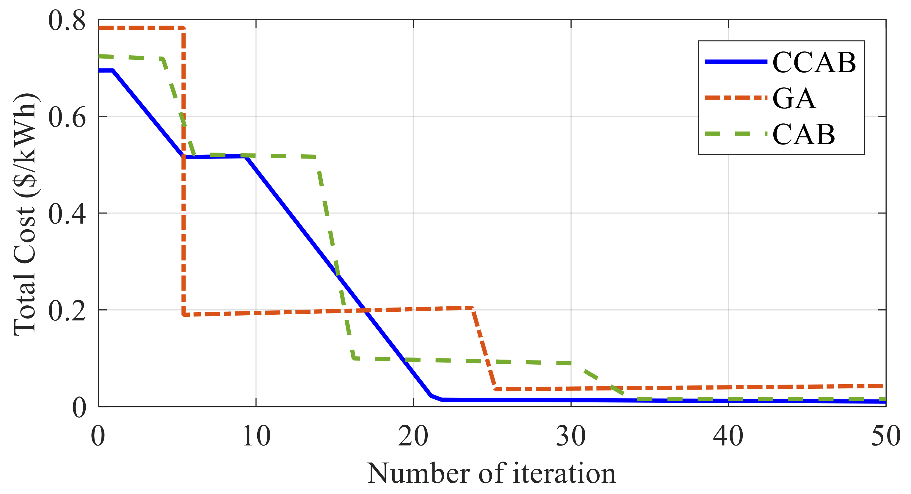
3.1. Calculation of Optimum Parameters

The model is developed with the objective function for minimizing the cost of fuel cell fabrication based on the proposed converged collective animal behavior (CCAB) algorithm and solving the optimal values for each of the main parameters. As can be observed, the optimal operating temperature is $75.2 °\mathrm{C}$, the optimal system pressure is approximately $0.47 \mathrm{MPa}$, the optimal density of the current is almost $0.61 \mathrm{mA}/{\mathrm{cm}}^2$, and the optimal stoichiometry coefficients are 1.42 for air and 1.25 for hydrogen.

Table 4. Optimal values for optimization parameters.

Algorithm	Parameter
	${\lambda }_{air}$	${\lambda }_{H_2}$	$P_{sys}$	$T$	$i$
CCAB	1.42	1.25	0.47	75.2	0.61
CAB	1.37	1.18	0.40	73.6	0.58
GA	1.10	1.20	0.32	72.4	0.55

indicates the optimal values for optimization parameters.

The optimal costs for the proposed CCAB, standard CAB, and GA are estimated at $0.1061 \$/\mathrm{kWh}$, $0.1124 \$/\mathrm{kWh}$, and $0.1603 \$/\mathrm{kWh}$. Figure 4 depicts the performance diagram of the optimizers in the optimization process. The results show how as time passes and the number of new iterations becomes more and more objective, the objective function shifts to the lowest feasible amount.

In the following, for the sensitivity analysis of the system performance, variables are repeatedly changed each time, but the values of the other parameters are replaced with the optimal values obtained by the CCAB algorithm.

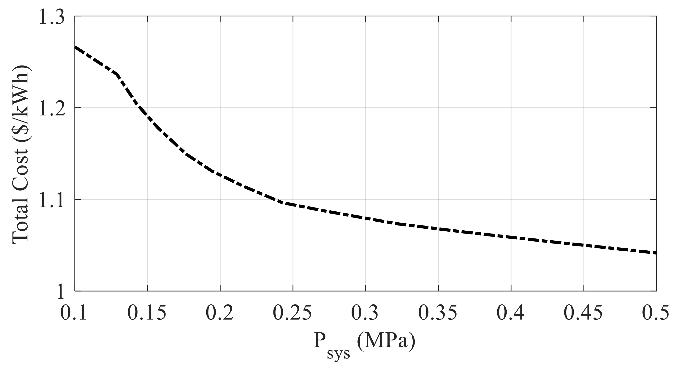
3.2. The Pressure Changes Affect the Construction Cost of the Cell

As can be concluded from the results of Figure 5, by increasing the inlet pressure of the system up to 5 bar, the total cost of it is decreased by 20%. However, this increase in pressure due to the mechanical and physical mechanisms of the membrane and the electrodes, and also the bipolar plates is not feasible. By the increase in pressure, also the linkages between the gas diffusion plates and the catalyst are eliminated, while the gas diffusion surfaces generally consist of carbon coatings or paper carbon, which are corrosive to the mechanism. Therefore, consideration of the structure of its constituents is adapted.

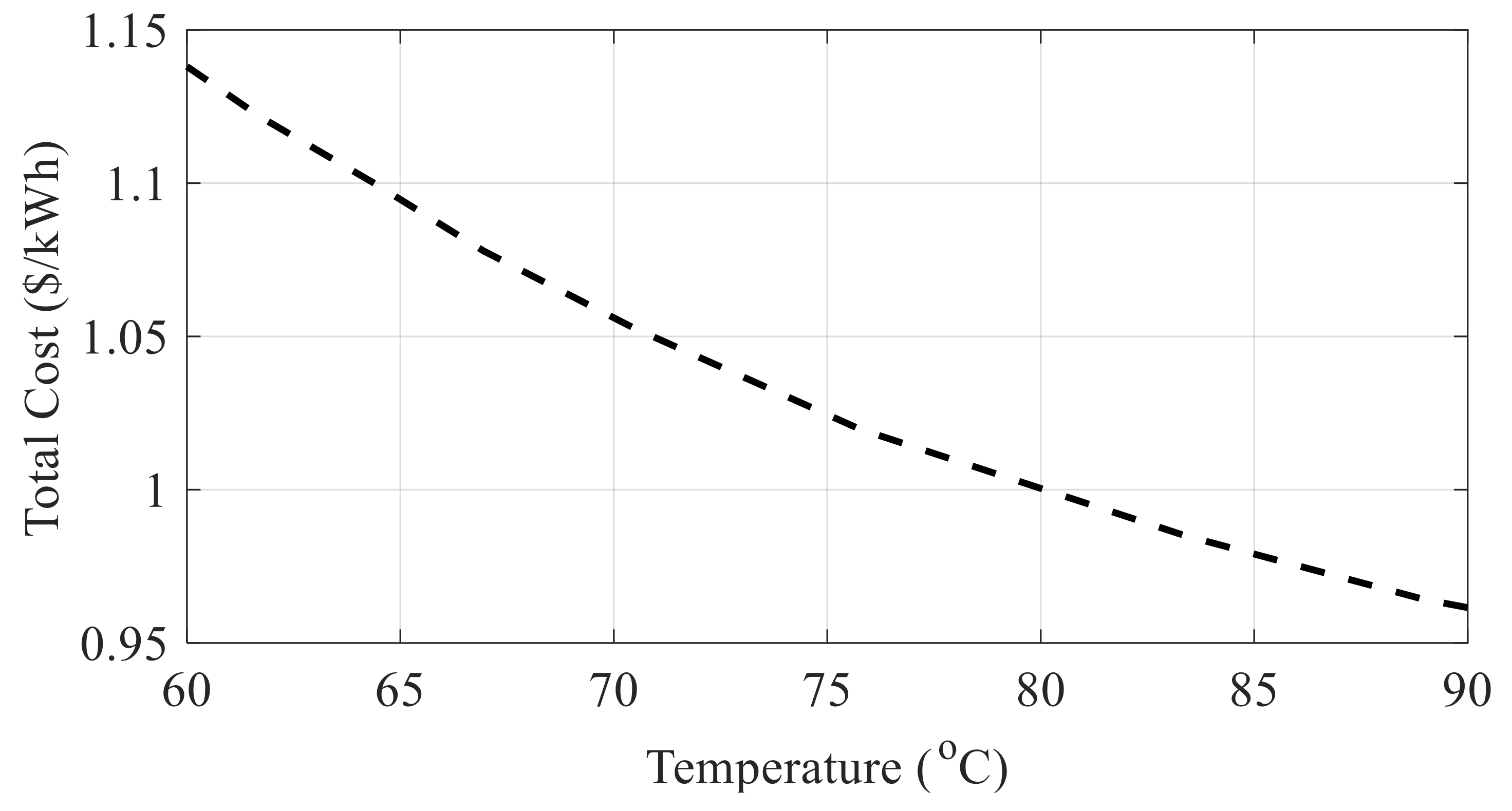
3.3. The Temperature Changes Affect the Construction Cost of the Cell

Assuming that the operating temperature of the fuel cell is variable and that the other modeling parameters are stable (their optimal value), the total cost of the system decreases with increasing temperature (Figure 6). However, two points need to be noted: firstly, Nafion’s heat resistance as a membrane of the fuel cell is a limiting element for the exceedingly high operation temperature, and the second is that the best way for the protons to pass by the membrane is when the water is moved in the two steps of the heater and operation fluid. The only water step in the fuel cell is the steam step if the peak operation temperature is increased, which has an impact on the hydrogen exchange. Therefore, the efficiency of the system is greatly reduced if all the parameters are affected. Therefore, by considering all of the effective parameters in the fuel cell performance as variables, the optimal mode for its operation is 75.2 °C. At this temperature, the membrane passing water is completely biphasic.

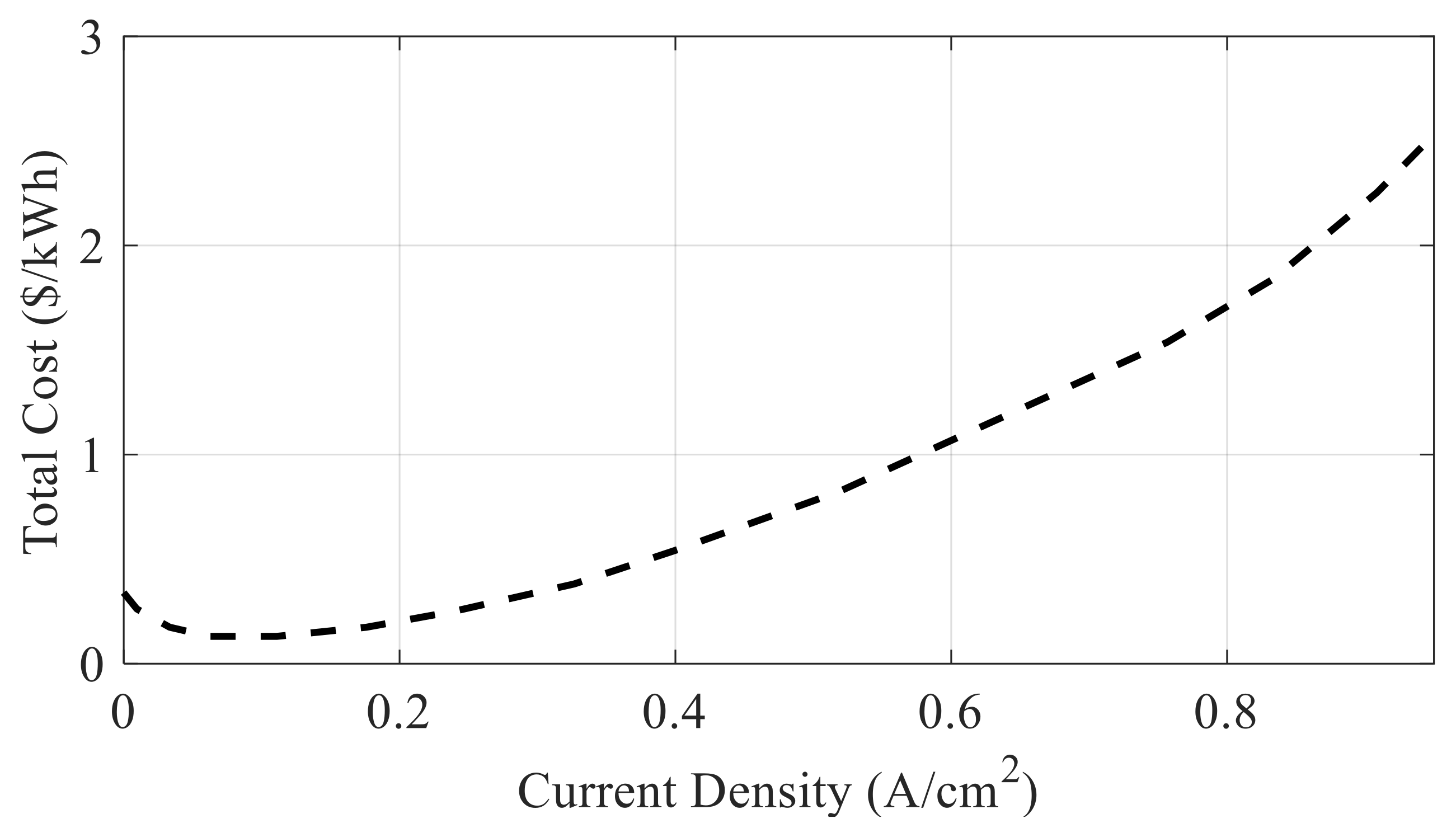
3.4. The Current Density Effect on the Construction Cost of the Cell

The total cost changes, as concerns the current density changes, are depicted in Figure 7. Notably, due to the relationships presented in the modeling section, it is not possible to directly modify the current density. However, investigations to find out how much the system is optimized for parameter changes indicate that the cost of the overall system is increased with an increase in the current density. This is because one of the most important methods to increase the porosity of the porous membrane–catalyst–porous current is to use rather cost-effective approaches when fabricating the membrane electrode group, so the optimal amount of this parameter based on the objective function is $0.61 \mathrm{mA}/{\mathrm{cm}}^2$.

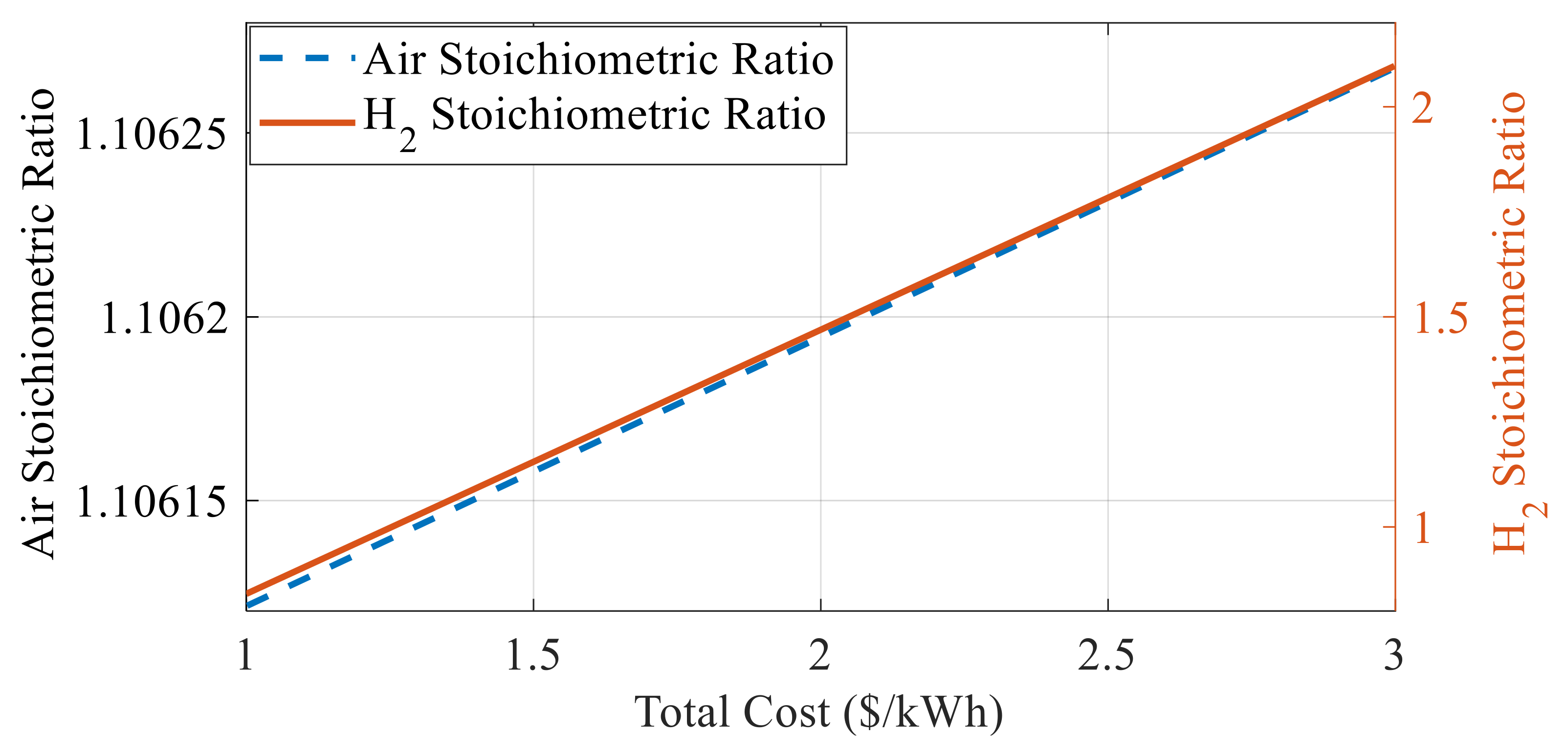
3.5. The Stoichiometric Coefficients of Hydrogen and Air Effect on the Construction Cost of the Cell

The following figure (Figure 8) depicts the changes in the total cost of the system of fuel cells relative to the changes in the stoichiometric coefficients of the reactants. As can be seen, in both forms, the cost of the process increases if the proportion of the stoichiometry is increased. The difference between them is that changes in the stoichiometric air ratio have a low pronounced effect on the hydrogen cost. This is also due to the high cost of construction, storage, and transport of hydrogen. Therefore, it is increased to obtain the optimal parameter values, but it is worth noting that when this ratio increases, which is directly proportional to the increase in the inlet air, the compressor power can be a factor limiting the cost reduction.

Finally, by considering all the cases, the impact of the entire efficiency of the system on the cost of the system is given in Figure 9. As can be seen, by improving the performance of the fuel cell, its total cost is decreased.

4. Conclusions

To directly convert chemical energy into electricity without combustion, an electrochemical device, which is called a fuel cell, is used. Because of the various benefits of this device, including cleanliness, connection to micro-turbines, silent operation, no moving elements, and lack of GHG emission, it has become a favored energy source recently. One of the biggest disadvantages of these energy conversion systems is their cost of construction and operation. This study attempted to find the best operating conditions in a 50 kW fuel cell stack to minimize its cost and its accessories, such as compressors and humidifiers. In this regard, a functional–economic model was developed for the system under study in which all components of the system are modeled economically as well as electrochemically–mechanically. The objective function here was solved by a newly improved metaheuristic by the authors called the converged collective animal behavior (CCAB) optimizer. The optimal cost was compared with standard CAB and GA, and the best optimal value was achieved by the CCAB with $0.1061 \$/\mathrm{kWh}$. Afterward, a sensitivity analysis was applied to the above-mentioned performance parameters. The results declare that as the temperature and the system pressure increases, the system cost decreases, but since the structure of the membrane and the fuel electrode must be considered in terms of thermal resistance and mechanical strength, limiting factors for their control and achieving optimal performance (higher efficiency) are to be taken into account. On the one hand, increasing the stoichiometric ratio of air and hydrogen increments the entire system cost, which is logical, given the conditions of production and storage of this transducer. At the same time, increasing the density of current initially decreases the costs and then increases it, which is due to the porosity of the triple layer of the membrane–electrocatalyst–gas diffusion plates, which can be calculated based on the performance parameters and the relations governing the economic–functional modeling and the change rate of the system relative to it.

References

1. Liu, J.; Gao, Y.; Yin, Y.; Wang, J.; Luo, W.; Sun, G. Introduction of Proton Exchange Membrane Fuel Cell Systems. In Sliding Mode Control Methodology in the Applications of Industrial Power Systems; Springer: Cham, Switzerland, 2020; pp. 63–82. [Google Scholar]
2. Nouri, A.; Khodaei, H.; Darvishan, A.; Sharifian, S.; Ghadimi, N. Optimal performance of fuel cell-CHP-battery based micro-grid under real-time energy management: An epsilon constraint method and fuzzy satisfying approach. Energy 2018, 159, 121–133. [Google Scholar] [CrossRef]
3. Khodaei, H.; Hajiali, M.; Darvishan, A.; Sepehr, M.; Ghadimi, N. Fuzzy-based heat and power hub models for cost-emission operation of an industrial consumer using compromise programming. Appl. Therm. Eng. 2018, 137, 395–405. [Google Scholar] [CrossRef]
4. Dehghani, M.; Ghiasi, M.; Niknam, T.; Kavousi-Fard, A.; Shasadeghi, M.; Ghadimi, N.; Taghizadeh-Hesary, F. Blockchain-based securing of data exchange in a power transmission system considering congestion management and social welfare. Sustainability 2021, 13, 90. [Google Scholar] [CrossRef]
5. Mirzapour, F.; Lakzaei, M.; Varamini, G.; Teimourian, M.; Ghadimi, N. A new prediction model of battery and wind-solar output in hybrid power system. J. Ambient. Intell. Humaniz. Comput. 2017, 10, 77–87. [Google Scholar] [CrossRef]
6. Ghadimi, N.; Ghadimi, R.; Danandeh, A. Applying Genetic Algorithm to Adjustment PID Coefficients in Order to Power Control of Micro-Turbine in Island Condition. Res. J. Inf. Technol. 2012, 4, 13–17. [Google Scholar]
7. Bao, C.; Bessler, W.G. Two-dimensional modeling of a polymer electrolyte membrane fuel cell with long flow channel. Part II. Physics-based electrochemical impedance analysis. J. Power Sources 2015, 278, 675–682. [Google Scholar] [CrossRef] [Green Version]
8. Solsona, M.; Kunusch, C.; Ocampo-Martinez, C. Control-oriented model of a membrane humidifier for fuel cell applications. Energy Convers. Manag. 2017, 137, 121–129. [Google Scholar] [CrossRef] [Green Version]
9. Bernardi, D.M.; Verbrugge, M.W. A mathematical model of the solid-polymer-electrolyte fuel cell. J. Electrochem. Soc. 1992, 139, 2477–2491. [Google Scholar] [CrossRef]
10. Hirano, S.; Shimpalee, S.; Lu, Z.; Satjaritanun, P.; Weidner, J.W. Investigation of PEMFC Performance and Property of the Gas Diffusion Layers Utilizing the Numerical Model. ECS Meet. Abstr. 2017, 1419. [Google Scholar] [CrossRef]
11. Taleb, M.A.; Béthoux, O.; Godoy, E. Identification of a PEMFC fractional order model. Int. J. Hydrog. Energy 2017, 42, 1499–1509. [Google Scholar] [CrossRef]
12. Kumar, P.A.; Geetha, M.; Chandran, K.; Sanjeevikumar, P. PEM Fuel Cell System Identification and Control. In Advances in Smart Grid and Renewable Energy; Springer: Berlin/Heidelberg, Germany, 2018; pp. 449–457. [Google Scholar]
13. Duan, B.; Cao, Q.; Afshar, N. Optimal parameter identification for the proton exchange membrane fuel cell using Satin Bowerbird optimizer. Int. J. Energy Res. 2019, 43, 8623–8632. [Google Scholar] [CrossRef]
14. Ariza, H.E.; Correcher, A.; Sánchez, C.; Pérez-Navarro, Á.; García, E. Thermal and electrical parameter identification of a proton exchange membrane fuel cell using genetic algorithm. Energies 2018, 11, 2099. [Google Scholar] [CrossRef] [Green Version]
15. Yang, Z.; Ghadamyari, M.; Khorramdel, H.; Alizadeh, S.M.S.; Pirouzi, S.; Milani, M.; Banihashemi, F.; Ghadimi, N. Robust multi-objective optimal design of islanded hybrid system with renewable and diesel sources/stationary and mobile energy storage systems. Renew. Sustain. Energy Rev. 2021, 148, 111295. [Google Scholar] [CrossRef]
16. Mehrpooya, M.; Ghadimi, N.; Marefati, M.; Ghorbanian, S.A. Numerical investigation of a new combined energy system includes parabolic dish solar collector, Stirling engine and thermoelectric device. Int. J. Energy Res. 2021, 45, 16436–16455. [Google Scholar] [CrossRef]
17. Hamal, N.; Isa, Z.; Nayan, N.; Arshad, M.; Kajaan, N. Optimizing PEMFC Model Parameters Using Dragonfly Algorithm: A Performance Study; IEEE: Kaula Lumpur, Malaysia, 2018. [Google Scholar]
18. Fathy, A.; Rezk, H. Multi-verse optimizer for identifying the optimal parameters of PEMFC model. Energy 2018, 143, 634–644. [Google Scholar] [CrossRef]
19. Misaghi, M.; Yaghoobi, M. Improved Invasive weed optimization Algorithm (IWO) Based on Chaos Theory for Optimal design of PID controller. J. Comput. Des. Eng. 2019, 6, 284–295. [Google Scholar] [CrossRef]
20. Brammya, G.; Praveena, S.; Preetha, N.S.N.; Ramya, R.; Rajakumar, B.R.; Binu, D. Deer Hunting Optimization Algorithm: A New Nature-Inspired Meta-heuristic Paradigm. Comput. J. 2019, bxy133. [Google Scholar] [CrossRef]
21. Arora, S.; Anand, P. Chaotic grasshopper optimization algorithm for global optimization. Neural Comput. Appl. 2019, 31, 4385–4405. [Google Scholar] [CrossRef]
22. Carton, J.; Olabi, A.G. Three-dimensional proton exchange membrane fuel cell model: Comparison of double channel and open pore cellular foam flow plates. Energy 2017, 136, 185–195. [Google Scholar] [CrossRef] [Green Version]
23. Yuan, Z.; Wang, W.; Wang, H.; Ghadimi, N. Probabilistic decomposition-based security constrained transmission expansion planning incorporating distributed series reactor. IET Gener. Transm. Distrib. 2020, 14, 3478–3487. [Google Scholar] [CrossRef]
24. Fathy, A.; Elaziz, M.A.; Alharbi, A.G. A novel approach based on hybrid vortex search algorithm and differential evolution for identifying the optimal parameters of PEM fuel cell. Renew. Energy 2020, 146, 1833–1845. [Google Scholar] [CrossRef]
25. Razmjooy, N.; Khalilpour, M.; Ramezani, M. A New Meta-Heuristic Optimization Algorithm Inspired by FIFA World Cup Competitions: Theory and Its Application in PID Designing for AVR System. J. Control. Autom. Electr. Syst. 2016, 27, 419–440. [Google Scholar] [CrossRef]
26. Razmjooy, N.; Ramezani, M. Improved Quantum Evolutionary Algorithm Based on Invasive Weed Optimization. Indian J. Sci. Res. 2014, 4, 413–422. [Google Scholar]
27. Liu, J.; Chen, C.; Liu, Z.; Jermsittiparsert, K.; Ghadimi, N. An IGDT-based risk-involved optimal bidding strategy for hydrogen storage-based intelligent parking lot of electric vehicles. J. Energy Storage 2020, 27, 101057. [Google Scholar] [CrossRef]
28. Grujicic, M.; Chittajallu, K. Design and optimization of polymer electrolyte membrane (PEM) fuel cells. Appl. Surf. Sci. 2004, 227, 56–72. [Google Scholar] [CrossRef]
29. Mahmoudi, S.M.S.; Sarabchi, N.; Yari, M.; Rosen, M.A. Exergy and Exergoeconomic Analyses of a Combined Power Producing System including a Proton Exchange Membrane Fuel Cell and an Organic Rankine Cycle. Sustainability 2019, 11, 3264. [Google Scholar] [CrossRef] [Green Version]
30. Tsuchiya, H.; Kobayashi, O. Mass production cost of PEM fuel cell by learning curve. Int. J. Hydrog. Energy 2004, 29, 985–990. [Google Scholar] [CrossRef]
31. Ahadi, A.; Ghadimi, N.; Mirabbasi, D. Reliability assessment for components of large scale photovoltaic systems. J. Power Sources 2014, 264, 211–219. [Google Scholar] [CrossRef]
32. Correa, J.; Farret, F.A.; Canha, L.; Simoes, M. An electrochemical-based fuel-cell model suitable for electrical engineering automation approach. IEEE Trans. Ind. Electron. 2004, 51, 1103–1112. [Google Scholar] [CrossRef]
33. Aouali, F.; Becherif, M.; Ramadan, H.; Emziane, M.; Khellaf, A.; Mohammedi, K. Analytical modelling and experimental validation of proton exchange membrane electrolyser for hydrogen production. Int. J. Hydrogen Energy 2017, 42, 1366–1374. [Google Scholar] [CrossRef]
34. Kandidayeni, M.; Macias, A.; Khalatbarisoltani, A.; Boulon, L.; Kelouwani, S. Benchmark of Proton Exchange Membrane Fuel Cell Parameters Extraction with Metaheuristic Optimization Algorithms. Energy 2019, 183, 912–925. [Google Scholar] [CrossRef]
35. Tizhoosh, H.R. Opposition-based learning: A new scheme for machine intelligence. In Proceedings of the International Conference on Computational Intelligence for Modelling, Control and Automation and International Conference on Intelligent Agents, Web Technologies and Internet Commerce (CIMCA-IAWTIC′06), Vienna, Austria, 28–30 November 2005; Volume 1, pp. 695–701. [Google Scholar]
36. Na, W.; Gou, B. The efficient and economic design of PEM fuel cell systems by multi-objective optimization. J. Power Sources 2007, 166, 411–418. [Google Scholar] [CrossRef]
37. Cui, Z.; Zhang, J.; Wang, Y.; Cao, Y.; Cai, X.; Zhang, W.; Chen, J. A pigeon-inspired optimization algorithm for many-objective optimization problems. Sci. China Inf. Sci. 2019, 62, 70212. [Google Scholar] [CrossRef] [Green Version]
38. Wang, G.-G.; Gao, X.-Z.; Zenger, K.; Coelho, L.D.S. A novel metaheuristic algorithm inspired by rhino herd behavior. In Proceedings of the 9th EUROSIM and the 57th SIMS, Oulu, Finland, 12–16 September 2018; Linköping University Electronic Press: Oulu, Finland; pp. 1026–1033.
39. Cuevas, E.; Reyna-Orta, A.; Cortes, M.A.D. A Multimodal Optimization Algorithm Inspired by the States of Matter. Neural Process. Lett. 2017, 48, 517–556. [Google Scholar] [CrossRef]
40. Kumar, M.; Kulkarni, A.; Satapathy, S.C. Socio evolution & learning optimization algorithm: A socio-inspired optimization methodology. Futur. Gener. Comput. Syst. 2018, 81, 252–272. [Google Scholar]
41. Bandaghiri, P.S.; Moradi, N.; Tehrani, S.S. Optimal tuning of PID controller parameters for speed control of DC motor based on world cup optimization algorithm. Parameters 2016, 1, 106–111. [Google Scholar]
42. Razmjooy, N.; Madadi, A.; Ramezani, M. Robust Control of Power System Stabilizer Using World Cup Optimization Algorithm. Int. J. Inf. Secur. Syst. Manag. 2017, 5, 519–526. [Google Scholar]
43. Shahrezaee, M. Image segmentation based on world cup optimization algorithm. Majlesi J. Electr. Eng. 2017, 11. Available online: http://mjee.iaumajlesi.ac.ir/index/index.php/ee/article/view/2213 (accessed on 13 November 2021).
44. Cuevas, E.; Fausto, F.; Gonzalez, A. A. A Swarm Algorithm Inspired by the Collective Animal Behavior. In New Advancements in Swarm Algorithms: Operators and Applications; Springer: Cham, Switzerland, 2020; pp. 161–188. [Google Scholar]
45. Yang, D.; Li, G.; Cheng, G. On the efficiency of chaos optimization algorithms for global optimization. Chaos Solitons Fractals 2007, 34, 1366–1375. [Google Scholar] [CrossRef]
46. Rim, C.; Piao, S.; Li, G.; Pak, U. A niching chaos optimization algorithm for multimodal optimization. Soft Comput. 2016, 22, 621–633. [Google Scholar] [CrossRef]
47. Dhiman, G.; Kumar, V. Emperor penguin optimizer: A bio-inspired algorithm for engineering problems. Knowl.-Based Syst. 2018, 159, 20–50. [Google Scholar] [CrossRef]
48. Rashedi, E.; Nezamabadi-Pour, H.; Saryazdi, S. GSA: A gravitational search algorithm. Inf. Sci. 2009, 179, 2232–2248. [Google Scholar] [CrossRef]
Figure 1. The overall configuration of the analyzed system.
Sustainability 13 12771 g001
Figure 2. The general structure of a PEMFC.
Sustainability 13 12771 g002
Figure 3. The workflow of the suggested CCAB algorithm.
Sustainability 13 12771 g003
Figure 4. The diagram of changes in objective function value by the number of iterations.
Sustainability 13 12771 g004
Figure 5. Final cost changes according to the system pressure.
Sustainability 13 12771 g005
Figure 6. Final cost changes according to the system pressure.
Sustainability 13 12771 g006
Figure 7. Final cost changes according to the system’s current density.
Sustainability 13 12771 g007
Figure 8. Final cost changes according to the system hydrogen and air stoichiometric coefficients.
Sustainability 13 12771 g008
Figure 9. The impact of the entire efficiency of the system on the cost of the system.
Sustainability 13 12771 g009