An Empirical Mode Decomposition for Establishing Spatiotemporal Air Quality Trends in Shandong Province, China

Abstract

Air pollution is a serious problem in China, and the government has taken a series of steps to solve it. However, it is still u2nclear how the situation has improved after years of atmospheric pollution control. Shandong Province, which has the second largest population and the highest coal consumption in China, was chosen to analyze the spatiotemporal air quality trends. We obtained daily air quality index (AQI) values from 91 stations in the province from 1 January 2014, to 31 December 2019, based on an adaptive data analysis method, empirical mode decomposition (EMD). The distribution of AQI in Shandong Province was heterogeneous at both spatial and temporal scales. All the stations could be divided into four clusters whose AQI trends decreased from 75 to 53, 95 to 68, 128 to 82, and 148 to 82, respectively. The overall trend of pollution became more serious from east to west in the province. The AQI is the largest in winter, followed by spring and autumn, and the smallest index occurs in summer. There are four types of annual trends of the AQI of each city. The overall downward trend indicates that the air quality of each city was improving annually.

1. Introduction

Frequent air pollution episodes have attracted the attention of the whole of China in recent years. Air pollution has severe impacts on human health, causing acute and chronic respiratory diseases and even leading to death [1,2,3,4]. Problems related to air pollution are increasing in many developing countries due to urbanization, industrial development, increasing use of cars, etc. [5]. The Chinese government has made great efforts to reduce air pollution, such as the Heavy Air Pollution Contingency Plan, 2017 Air Pollution Prevention and Management Plan for the Beijing–Tian–Hebei region and its Surrounding Areas [6,7]. Several studies analyzed the change in separate pollutants in China in recent years [8,9]. However, after years of air pollution control, concern remains regarding how much the general air pollution situation has improved in the country. Air quality can be evaluated both by using air quality models [10,11] and by ground-based monitoring data at different scales. The air quality index (AQI) is an important comprehensive indicator used to measure air quality. The main pollutants involved in air quality assessment include fine particles (PM_2.5), coarse particulate matter (PM₁₀), sulfur dioxide (SO₂), nitrogen dioxide (NO₂), ozone (O₃), and carbon monoxide (CO). By discovering the spatial and temporal distributions of AQI values, effective measures can be implemented to reduce air pollution. Spatial characteristics are helpful in finding the spatial distribution patterns of the AQI, while time series features can be used to find the period and trend of the AQI. Therefore, in this study, we aim to evaluate the general air pollution trend and spatial difference in China with dozens of stations’ daily AQI data in Shandong, the second largest province.

Shandong is the province with the highest coal consumption in China. In the past 30 years, it has produced the highest sulfur dioxide emissions in China. Since 2010, Shandong has been committed to the management of air pollution. In 2013, it issued and started the “Shandong Province 2013–2020 Air Pollution Prevention and Control Plan” and put forward the idea of “one goal, three articles and six measures” for air pollution prevention and control. Shandong has a clear road map and timetable for “the dream of spanning eight years in the blue sky”. At the same time, Shandong issued and implemented the “Shandong Regional Comprehensive Emission Standards for Atmospheric Pollutants”, and control was gradually tightened for five key industries, including thermal power, iron and steel, boilers, building materials, and industrial furnaces and kilns, in four periods over eight years. However, air pollution in Shandong Province is still relatively serious and is restricting the sustainable and healthy development of Shandong’s economy. Therefore, in this study, we provide a scientific basis for air pollution control decision making and pollution prevention by analyzing the status quo of the seasonal and annual variation characteristics of air quality in Shandong Province and exploring the main influencing factors of air pollution, which is also helpful for the environmental protection administrative departments.

2. Methods

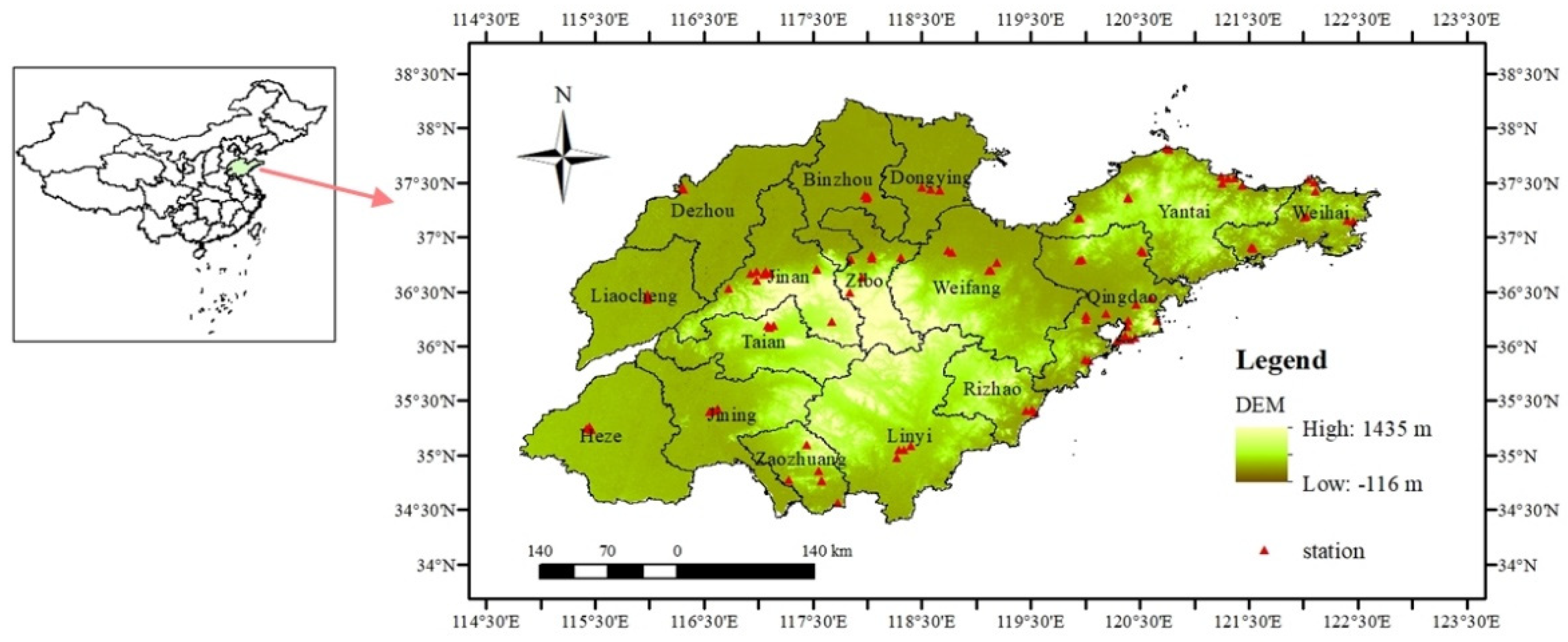
2.1. Data Source

There are 16 prefecture-level cities in Shandong Province. We obtained the daily air pollution index (AQI) and major contaminant types from 1 January 2014, to 31 December 2019, from the online air quality data website maintained by the China National Environmental Monitoring Center. The monitored pollutants included PM_2.5, PM₁₀, SO₂, NO₂, O₃ and CO. For each station, the daily AQI of each pollutant was calculated on the basis of a 24-h average. The AQI was the daily maximum value of the air quality sub-index of each pollutant. The AQI value characterized the degree of overall pollution, but not the concentrations of specific contaminants. The six pollutants used to calculate the AQI usually had different concentration limits. During the calculation, each pollutant was converted into an air quality sub-index of the AQI according to the different target concentration limits. The AQI was divided into the six levels of 0–50, 51–100, 101–150, 151–200, 201–300 and greater than 300, corresponding to six levels of air quality [12]. The higher the index was, the higher the level, indicating that the pollution was more severe. There were 91 survey stations distributed in 16 cities of Shandong Province (Figure 1). In Shandong, spring includes March, April, and May; summer is June, July, and August; autumn is September, October, and November; and winter includes December, January and February (the following year).

We calculated the daily index of each pollutant by the measured concentrations of the six pollutants according to the concentration limit of each pollutant as follows (GB3095-2012, GB3095-1996):

$${\mathrm{IAQI}}_i=\frac{I_{high}-I_{low}}{C_{high}-C_{low}}\left(C-C_{low}\right)+I_{low}$$

(1)

where IAQI_i is the individual air quality index of the ith pollutant; C is the mass concentration of the pollutant; C_high is the concentration breakpoint that is >C; C_low is the breakpoint that is ≤C; and I_high and I_low are the individual air quality indexes corresponding to C_high and C_low, respectively. The AQI is the maximum value of IAQI_i:

$$\mathrm{AQI}=\max \left\{{\mathrm{IAQI}}_1,{\mathrm{IAQI}}_2,{\mathrm{IAQI}}_3,\cdots ,{\mathrm{IAQI}}_{\mathrm{n}}\right\}$$

(2)

2.2. Temporal Period and Trend Decomposition

For the daily AQI, there are 2191 days recorded at each station from 1 January 2014, to 31 December 2019. We divided the 2191 days into 312 weeks to obtain the weekly average value. We clustered the 91 sites by a K-means algorithm based on the time series of the AQI. Then, the empirical mode decomposition (EMD) method was used to decompose the time series of each cluster and analyze its time periodicity and trend.

For the air pollution dataset $\left\{x^{\left(1\right)},\cdots ,x^{\left(91\right)}\right\},x^{\left(i\right)}\in {ℝ}^n$, the stations are classified into K classes based on the similarity of daily AQIs measured by the Euclidean distance in high-dimension spaces [13]. After determining the K value based on the often-adopted elbow method [14], we used the statistical software R 4.0 [15] and the package kernlab [16] to run the clustering method.

The empirical mode decomposition (EMD) method proposed by Huang et al. is based on the time scale for signal decomposition, which is different from the Fourier decomposition and wavelet decomposition methods [17,18]. The latter two methods are based on a priori basis functions, while the EMD method does not need to preset any basis function. So, the EMD method can be used to decompose both stationary and nonstationary signals. This decomposition is adaptively based on the local characteristics of the time scale of the signal sequence [19]. It decomposes the fluctuation of a time series on different scales and generates a series of data with different characteristic scales, called an intrinsic mode function (IMF). Then, a signal can be decomposed into several IMFs and a trend item. An IMF satisfies two conditions. First, the difference of the number of local maxima (or minima) and the number of zero-crossing points in an IMF is zero or one. Second, the mean of the envelope defined by the local maxima $e_{max}\left(t\right)$ and the envelope defined by the local minima $e_{min}\left(t\right)$ is zero at any local point.

For the time series AQI data $x\left(t\right)$, the EMD steps are as follows:

First, we find all extreme points of $x\left(t\right)$, which is the weekly AQI series.

Second, for $x\left(t\right)$, a cubic point function is used to fit the maximum point to the upper envelope $e_{max}\left(t\right)$, and then the minimum point is fitted to the lower envelope $e_{min}\left(t\right)$. The mean $m_1$ is calculated by Formula (3).

$$m_1=\frac{e_{max}\left(t\right)+e_{min}\left(t\right)}{2}$$

(3)

Third, by subtracting the above mean from the time series data $x\left(t\right)$, a new time series data point $c_1\left(t\right)=x\left(t\right)-m_1\left(t\right)$ can be obtained. The process is repeated until $c_1\left(t\right)$ meets the definition of the IMF. Then, the first IMF component $c_1\left(t\right)$ is obtained, which is the highest frequency component of the signal $x\left(t\right)$.

Fourth, by separating $c_1\left(t\right)$ from $x\left(t\right)$, we can obtain a difference signal $r_1\left(t\right)$ with the high-frequency component removed, as shown in Formula (4).

$$r_1\left(t\right)=x\left(t\right)-c_1\left(t\right)$$

(4)

Let $x\left(t\right)=r_1\left(t\right)$ and repeat the above steps to obtain the next IMF component. The process stops when no IMF can be found. Generally, this procedure is repeated n times to obtain n IMF components, as shown in Formula (5).

$$\left\{\begin{array}{c}{r}_1\left(t\right)-c_2\left(t\right)=r_2\left(t\right)\\ \dots \dots \\ r_{n-1}\left(t\right)-c_n\left(t\right)=r_n\left(t\right)\end{array}\right.$$

(5)

The last item, $r_n\left(t\right)$, is the residual term, indicating the overall trend of the signal. The IMF components, $c_i\left(t\right)$, contain the components of signals at different time scales, with periodic oscillations from fast to slow. The relationship between the original time-series data point $x\left(t\right)$, decomposed IMF $c_i\left(t\right)$ and the overall trend $r_n\left(t\right)$ can be expressed as Equation (6):

$$x\left(t\right)={{\displaystyle \sum }}_{i=1}^n{c}_i\left(t\right)+r_n\left(t\right)$$

(6)

We used the code written by Rilling to run the EMD method and used a cubic spline interpolation method for envelope fitting [20].

3. Results

3.1. Overview of the Data Set

The weekly average AQI values of the 91 stations from 2014 to 2019 varied greatly, ranging from less than 20 to more than 300 (Table S1 in Supplementary Material). A comparison of the median and mean AQI values showed that the data were slightly right-skewed for the 312 weeks. As shown in Table S1, in the column of the minimum AQI average value, 35 stations had AQI average values less than 25, and 27 of them belonged to three cities, i.e., Weihai, Qingdao, and Yantai. These three cities are located on the eastern coast and have well-developed economies. There were seven stations with weekly average AQI values greater than 350. These were mainly located in the northwest of Shandong Province. A total of 38.46% of the stations have an average AQI greater than 100.

The proportions of stations meeting the national level I (0–50), II (51–100), III (101–150), IV (151–200), V (201–300), and VI (greater than 300) standards were 15.08%, 53.44%, 21.95%, 6.76%, 2.65%, and 0.12%, respectively. The percentages of different standards varied greatly among the stations, and there was a large gap among the stations. Laishan EPA in Yantai had reached 95.83% of the excellent standards (level I and II standards). However, only 39.42% of the Provincial Seed Warehouse stations in Jinan met the excellent standards.

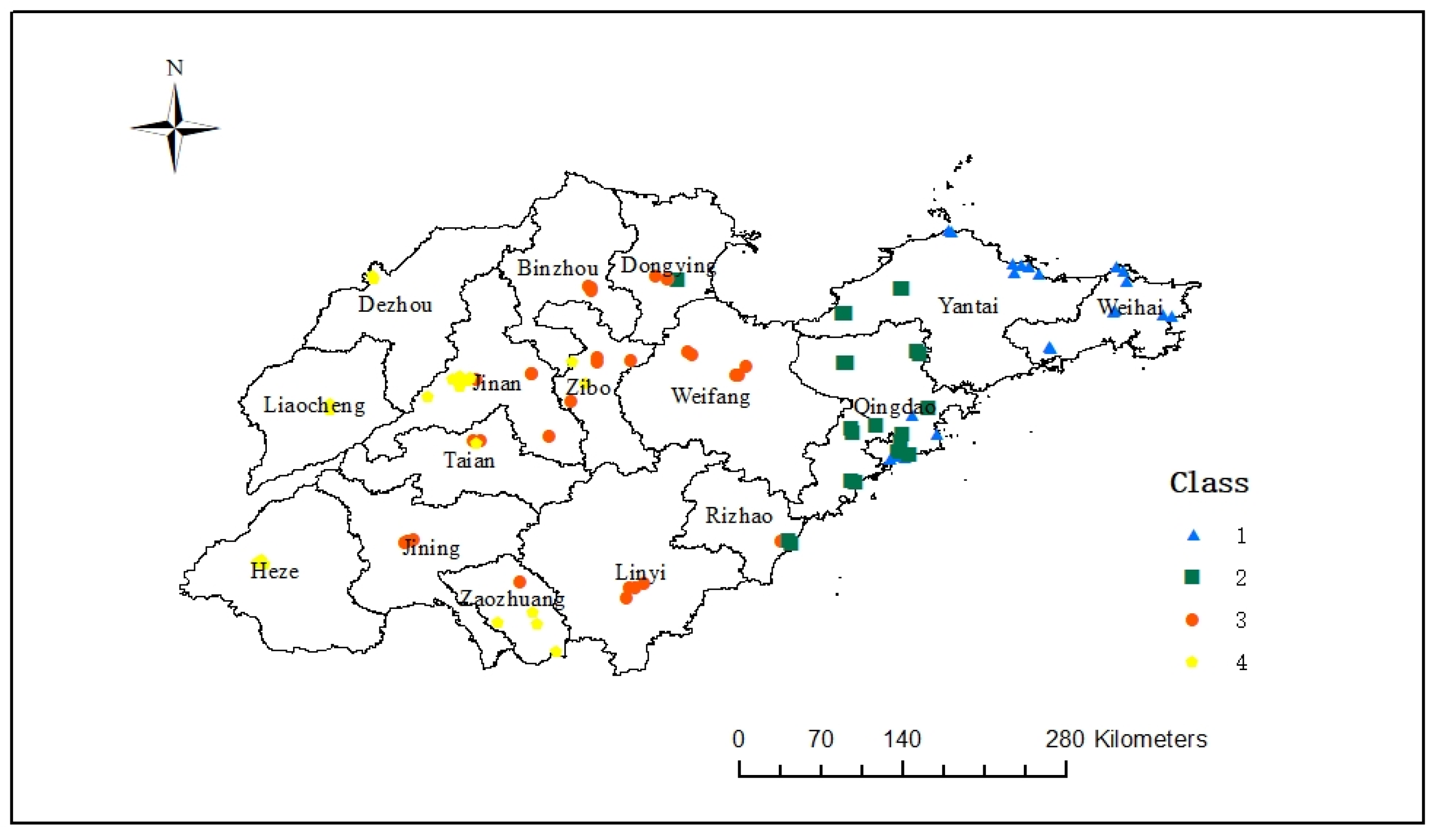
3.2. Spatial Distribution of Station Clustering

By K-means clustering, 91 stations were divided into four clusters (Figure 2). The first group includes 21 stations distributed in the eastern coastal cities of Shandong Province. The second group includes 21 stations located in the eastern and central cities of Shandong Province. The third group includes 29 stations mainly located in the central region of Shandong Province. The fourth group consists of 20 stations mainly located in western cities of Shandong Province. The pollution of the first cluster was the lowest, and the pollution of the fourth cluster was the most serious. The overall change trend was that the pollution becomes more serious when moving to the west.

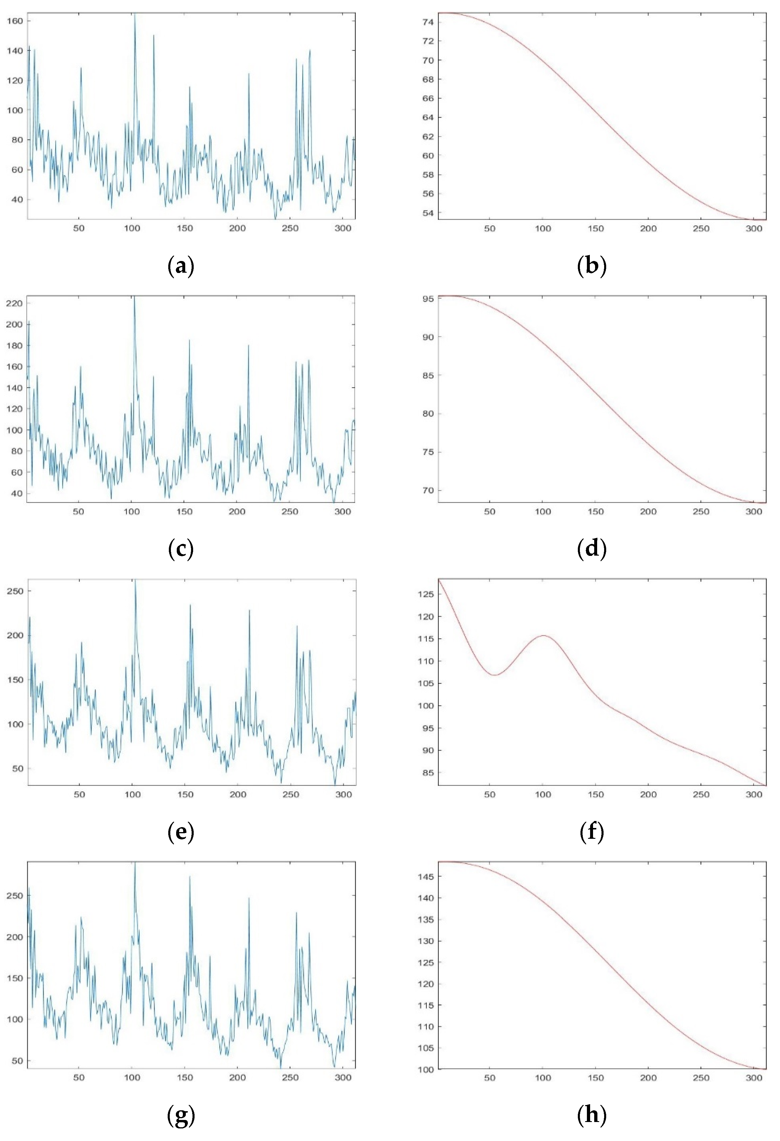
3.3. Temporal Trend of the AQI

The four cluster centers were decomposed by the EMD method to extract different temporal scale variations and global trends (Figure 3 and Figure S1 in the Supplementary Material). The first and second clusters generated six and seven IMFs, respectively. The remaining two clusters generated five IMFs. The decomposition results looked similar but differ in frequency and amplitude. IMF₁ had the highest frequency and maximum amplitude among the several IMFs, while the last IMF had the lowest frequency and minimum amplitude. The four cluster centers trended downward, indicating that the AQI value is decreasing. The trend ranges of the four cluster centers were 75 to 53, 95 to 68, 128 to 82 and 148 to 82, respectively. The trend of the fourth cluster center has a maximum decrease of 45%. Next is the third cluster center, which decreases by 36%. Another difference among the trends for the four cluster centers is the shape of the trend lines. For the first cluster, the trend remained stable from the first week to the 10th week (January 2014–March 2014), decreased uniformly from the 10th week to the 300th week (March 2014–October 2019), and remained stable from the 300th to 312th weeks (October 2019–December 2019). In contrast to that of the first cluster, the trend for the second cluster remained stable from the first week to the 20th week (January 2014–May 2014). For the third cluster, there was a rapid decrease from the first week to the 50th week (January 2014–December 2014), the trend rapidly increased from the 50th week to the 100th week (December 2014–December 2015), and it greatly decreased from the 100th week to the 312th week (December 2014–December 2019). For the fourth cluster, the rate of decrease was slow from the first week to the 50th week (January 2014–December 2014), with a uniform decline from the 50th week to the 300th week (December 2014–October 2019); the rate of decrease slowed down from the 300th to 312th weeks (October 2019–December 2019) and finally stabilized.

The AQI values vary greatly in different seasons. In the decomposition results, the period of IMF₅ is approximately one year. From IMF₁ to IMF₄, the period is less than one year, while IMF₆ and IMF₇ show inter-annual variation. We reconstructed the original series by summing the residuals and the IMFs without IMF₆ and IMF₇ to explore the seasonal variation in AQI values in the four clusters. On the basis of the four reconstructed datasets, the seasonal variation in the AQI is found by calculating the average AQI of each season in a cluster.

Among the four seasons, the AQI values in winter are the largest, much higher than those in other seasons, followed by spring, autumn, and summer. In spring, the change in the AQI index is slower and tends to decrease gradually. In summer, the AQI index was the largest in 2014, then decreased to 2016, when then there was an increasing trend, and it gradually decreased after 2017. In autumn, the AQI index continued to decrease gradually after 2016. In winter, the AQI index increased slowly from 2014 to 2015, decreased slowly after 2015, and gradually increased from 2017 to 2018.

3.4. Spatial Pattern of the Temporal Trend of Mass Concentration at Stations

We calculated the average AQI values of each city and extracted the annual trend of the AQI values of each city using the EMD method (Figure 4). A statistical test of nonlinear trends shows that all 16 trends obtained by decomposition showed nonlinear characteristics. Among all the cities, the three cities with the largest changes in index values were Dezhou (61.09), Jining (56.26) and Liaocheng (55.04). Tai’an (17.39) had the smallest change in index value, followed by Qingdao city (17.51).

According to the change types of the trend lines, four main types were decomposed in the 16 trends. The first type (I, decline) was monotonically decreasing and includes nine cities: Binzhou, Dongying, Jining, Liaocheng, Linyi, Taian, Weihai, Zaozhuang and Zibo. The second type was starting to increase and then decreased and includes five cities: Dezhou, Heze, Jinan, Rizhao, and Yantai (II, rise–decline). The third type was monotonically decreasing, then slightly rising, and then decreasing again (III, decline–rise–decline). The fourth type was monotonically decreasing and finally saw a small increase (IV, decline–rise). Qingdao belongs to this category. In Shandong Province, type I was the dominant type, accounting for 56.3% of all cities. The final trends of I, II, and III were similar, all decreasing, accounting for 93.8%.

4. Discussion

Based on the daily records of 91 stations in a typical province, we evaluated the general status of air pollution in China by analyzing the spatial and temporal characteristics of AQI. The average AQI value of the 91 stations for the 6 years was 95.36, which corresponds to national air quality standard II. While the air quality in Shandong Province was gradually improving, air pollution was still serious.

The spatial clustering of the 91 stations revealed the spatial heterogeneity of AQI values in Shandong Province. Air pollution was distributed with a gradient from east to west. The AQI values of the eastern coastal cities are the smallest, and the AQI values increase when moving westward. The cities of Heze, Liaocheng, and Dezhou in the northwest of Shandong Province are close to Kaifeng city in Henan Province and Handan and Xingtai in Hebei Province, whose air quality was not very good during the research periods. In autumn and winter, pollutants are easily transferred to those areas from nearby cities because northwest winds prevail at that time [21]. The central area of Shandong Province, including Linyi, Jinan, Zibo, and Tai’an, is mountainous, with high altitude. The diffusion of air pollutants is hindered in the western cities, and pollutants easily accumulate. As a result, the air pollution in Heze, Liaocheng, Dezhou, and the mountainous areas in central China is serious, with a high AQI index. However, the eastern coastal cities are more developed and invest more in environmental governance. Additionally, the wind speed is larger in the coastal cities, which is conducive to the diffusion of pollutants in the air, so the average AQI index is smaller.

Results showed that the time-series data decomposition method, EMD, is effective in air quality trend analysis. It is becoming a popular model in long-term air quality evaluation. Luo et al. researched the trends and seasonality of PM2.5 concentrations by EMD in the US and evaluated the simulation results of the air quality model [22]. The method was also used to predict particulate matter concentration by Fu et al. and achieved a prediction accuracy of approximately 80% [23]. The spatial and temporal patterns and trends show that the AQI values have gradually been decreasing in recent years. With the management and control of pollution emission sources over the years, the level of air pollution in the province has been reduced simultaneously. This might indicate that these protective measures of reducing the number of pollution sources are effective in reducing air pollution [24]. In 2014, Shandong Province launched a “heavy punch” for air pollution. First, the progress of a denitration project in the thermal power and cement industry was significantly accelerated. Rare earth denitrification catalysts have been industrialized through a large number of experiments. Additionally, standards for denitrification catalysts have been issued and implemented. In 2014, 24,528 MW of coal-fired power units in Shandong Province completed the denitrification transformation. Second, progress has been made in coal-fired desulfurization and dust removal. In 2014, coal-fired power units in Shandong Province achieved desulfurization for 3379 MW and dust removal for 18,873 MW. Except for long-term shutdowns, all 8370 square meters of iron and steel sintering machines that should be treated have achieved a desulfurization transformation. Third, the backward production capacity that affects environmental quality has been eliminated. In 2014, Qingdao closed 157 illegal sand washing plants and stone factories and Zibo shut down eight small thermal power units and regulated 655 enterprises, which involved power, steel, coking, cement, pottery, refractory, and other industries. A total of 810 sets of equipment for environmental management were newly built and renovated. Fourth, the task of eliminating small coal-fired boilers and changing coal into gas has been completed. In 2014, 5149 small coal-fired boilers, including earth-fired heating furnaces (5479.28 tons of steam), were eliminated in Shandong Province, and the task of eliminating small coal-fired boilers was over-fulfilled. Fifth, positive progress has been made in the prevention and control of dust pollution in industrial enterprises. Municipalities have strengthened the management of industrial stockyards. Most coal yards and stockyards have installed wind and dust suppression devices or regular sprinkler facilities, which has brought the unorganized emissions of dust from large industrial enterprises under obvious control. Sixth, the work of banning straw burning has achieved good results. The burning levels in the summer and autumn of 2014 decreased by 252 and 151, respectively, compared with the same period in 2013, with decreases of 52.39% and 60.4%, respectively. Seventh, the progress of technology has played an important role in environmental governance. In 2014, ultra-low emission technology in Shandong Province reached the national leading level, with the largest unit reaching 1 million kilowatts. Additionally, technical regulations and monitoring methods have been formulated for ultra-low emission monitoring, and relevant technical specifications have been promulgated, which is a first in China.

5. Conclusions

Using the EMD method, we effectively deconstructed the air quality trends in Shandong Province in recent years. The results showed that the air pollution control measures in the province in recent years have had significant effects in improving the air quality. Although the improvement is more pronounced in the western region of the province than that in the eastern region, air pollution is still high in the western region. On the one hand, the government sector needs to continue to impose strict restrictions on high pollution emission sources in the western region, including industrial sources, mobile sources, dust sources, biomass incineration, and agricultural and livestock sources. On the other hand, the restrictions should be strengthened in the western cities to formulate joint emission control measures at the regional level. A potential shortcoming of this paper is that we failed to collect time-series data on the variation of pollution emissions. Quantitatively establishing the relationship between pollution emissions and air quality requires further research.

References

- Lelieveld, J.; Evans, J.S.; Fnais, M.; Giannadaki, D.; Pozzer, A. The contribution of outdoor air pollution sources to premature mortality on a global scale. Nature 2015, 525, 367–371. [Google Scholar] [CrossRef] [PubMed]
- Wu, S.; Deng, F.; Huang, J.; Wang, H.; Shima, M.; Wang, X.; Qin, Y.; Zheng, C.; Wei, H.; Hao, Y. Blood Pressure Changes and Chemical Constituents of Particulate Air Pollution: Results from the Healthy Volunteer Natural Relocation (HVNR) Study. Environ. Health Perspect. 2013, 121, 66–72. [Google Scholar] [CrossRef] [PubMed]
- Qiu, H.; Yu, T.S.; Tian, L.; Wang, X.; Tse, L.A.; Wong, T. Effects of Coarse Participate Matter on Emergency Hospital Admissions for Respiratory Diseases: A Time-Series Analysis in Hong Kong. Environ. Health Perspect. 2012, 120, 572–576. [Google Scholar] [CrossRef] [PubMed] [Green Version]
- Brook, R.D.; Rajagopalan, S.; Pope, C.A.; Brook, J.R.; Kaufman, J.D. Particulate matter air pollution and cardiovascular disease: An update to the scientific statement from the American Heart Association. Circulation 2010, 121, 2331–2378. [Google Scholar] [CrossRef] [PubMed] [Green Version]
- Hu, M.; Jia, L.; Wang, J.; Pan, Y. Spatial and temporal characteristics of particulate matter in Beijing, China using the Empirical Mode Decomposition method. Sci. Total Environ. 2013, 458–460, 70–80. [Google Scholar] [CrossRef] [PubMed]
- Chen, Z.; Chen, D.; Wen, W.; Zhuang, Y.; Kwan, M.P.; Chen, B.; Zhao, B.; Yang, L.; Gao, B.; Li, R. Evaluating the “2+26” regional strategy for air quality improvement during two air pollution alerts in Beijing: Variations in PM2.5 concentrations, source apportionment, and the relative contribution of local emission and regional transport. Atmos. Chem. Phys. 2019, 19, 6879–6891. [Google Scholar] [CrossRef] [Green Version]
- Song, C.; Wu, L.; Xie, Y.; He, J.; Chen, X.; Wang, T.; Lin, Y.; Jin, T.; Wang, A.; Liu, Y. Air pollution in China: Status and spatiotemporal variations. Environ. Pollut. 2017, 227, 334–347. [Google Scholar] [CrossRef] [PubMed]
- Zhang, Q.; Zheng, Y.; Tong, D.; Shao, M.; Hao, J. Drivers of improved PM 2.5 air quality in China from 2013 to 2017. Proc. Natl. Acad. Sci. USA 2019, 116, 201907956. [Google Scholar] [CrossRef] [PubMed] [Green Version]
- Liu, Q.; Wang, S.; Zhang, W.; Jiaming, L.; Dong, G. The effect of natural and anthropogenic factors on PM2.5: Empirical evidence from Chinese cities with different income levels. Sci. Total Environ. 2019, 653, 157–167. [Google Scholar] [CrossRef] [PubMed]
- Wolf, T.; Pettersson, L.H.; Esau, I. A very high-resolution assessment and modelling of urban air quality. Atmos. Chem. Phys. 2020, 20, 625–647. [Google Scholar] [CrossRef] [Green Version]
- Thunis, P.; Clappier, A.; Pisoni, E.; Degraeuwe, B. Quantification of non-linearities as a function of time averaging in regional air quality modeling applications. Atmos. Environ. 2015, 103, 263–275. [Google Scholar] [CrossRef]
- China, M. Ambient Air Quality Standards (GB 3095-2012); China Environmental Science Press: Beijing, China, 2012. Available online: http://english.mee.gov.cn/Resources/standards/Air_Environment/quality_standard1/201605/t20160511_337502.shtml (accessed on 10 April 2020).
- Jain, A.K. Data clustering: 50 years beyond K-means. Pattern Recogn. Lett. 2010, 31, 651–666. [Google Scholar] [CrossRef]
- Joshi, K.D.; Nalwade, P.S. Modified K-Means for Better Initial Cluster Centres. Int. J. Comput. Sci. Mob. Comput. 2013, 2, 219–223. [Google Scholar]
- R Core Team. R: A Language and Environment for Statistical Computing; R Foundation for Statistical Computing: Vienna, Austria, 2012; Available online: https://www.r-project.org/ (accessed on 5 March 2020).
- Karatzoglou, A.; Smola, A.; Hornik, K.; Zeileis, A. Kernlab—An S4 Package for Kernel Methods in R. J. Stat. Softw. 2004, 11, 1–20. [Google Scholar] [CrossRef] [Green Version]
- Huang, N.; Wu, M.; Long, S.R.; Shen, S.; Qu, W.; Gloersen, P.; Fan, K.L. A confidence limit for the empirical mode decomposition and Hilbert spectral analysis. Proc. R. Soc. Lond. A 2003, 459, 2317–2345. [Google Scholar] [CrossRef]
- Huang, N.; Shen, Z.; Long, S.R.; Wu, M.C.; Shih, H.H.; Zheng, Q.; Yen, N.C.; Tung, C.C.; Liu, H.H. The empirical mode decomposition and the Hilbert spectrum for nonlinear and non-stationary time series analysis. Proc. R. Soc. Lond. A 1998, 454, 903–995. [Google Scholar] [CrossRef]
- Cheng, J.; Yu, D.; Yu, Y. Research on the intrinsic mode function (IMF) criterion in EMD method. Mech. Syst. Signal Process 2006, 20, 817–824. [Google Scholar]
- Rilling, G.; Flandrin, P.; Goncalves, P. On empirical mode decomposition and its algorithms. In Proceedings of the IEEE-EURASIP Workshop on Nonlinear Signal and Image Processing, Grado, Italy, 8–11 June 2003; Available online: https://hal.inria.fr/inria-00570628/en/ (accessed on 25 May 2020).
- He, J. Analysis on the Temporal and Spatial Distribution, Meteorological Impact and Health Risk of Air Pollutants in Shandong Province. Master’s Thesis, Nanjing University of Information Science and Technology, Nanjing, China, 2018. [Google Scholar]
- Luo, H.; Astitha, M.; Hogrefe, C.; Mathur, R.; Rao, S.T. Evaluating trends and seasonality in modeled PM2.5 concentrations using empirical mode decomposition. Atmos. Chem. Phys. 2020, 20, 13801–13815. [Google Scholar] [CrossRef]
- Fu, M.; Le, C.; Fan, T.; Prakapovich, R.; Manko, D.; Dmytrenko, O.; Lande, D.; Shahid, S.; Yaseen, Z.M. Integration of complete ensemble empirical mode decomposition with deep long short-term memory model for particulate matter concentration prediction. Environ. Sci. Pollut. Res. 2021. [Google Scholar] [CrossRef]
- Jiao, L. Environmentally Air Quality of Shandong Province Improving Year-on-Year in 2014. Available online: http://www.iqilu.com/html/zdys/news/2015/0518/2408238.shtml2015 (accessed on 25 October 2021).
Publisher’s Note: MDPI stays neutral with regard to jurisdictional claims in published maps and institutional affiliations. |
© 2021 by the authors. Licensee MDPI, Basel, Switzerland. This article is an open access article distributed under the terms and conditions of the Creative Commons Attribution (CC BY) license (https://creativecommons.org/licenses/by/4.0/).
Share and Cite
Wu, H.; Hu, M.; Zhang, Y.; Han, Y. An Empirical Mode Decomposition for Establishing Spatiotemporal Air Quality Trends in Shandong Province, China. Sustainability 2021, 13, 12901. https://doi.org/10.3390/su132212901
Wu H, Hu M, Zhang Y, Han Y. An Empirical Mode Decomposition for Establishing Spatiotemporal Air Quality Trends in Shandong Province, China. Sustainability. 2021; 13(22):12901. https://doi.org/10.3390/su132212901
Chicago/Turabian StyleWu, Huisheng, Maogui Hu, Yaping Zhang, and Yuan Han. 2021. "An Empirical Mode Decomposition for Establishing Spatiotemporal Air Quality Trends in Shandong Province, China" Sustainability 13, no. 22: 12901. https://doi.org/10.3390/su132212901
APA StyleWu, H., Hu, M., Zhang, Y., & Han, Y. (2021). An Empirical Mode Decomposition for Establishing Spatiotemporal Air Quality Trends in Shandong Province, China. Sustainability, 13(22), 12901. https://doi.org/10.3390/su132212901