Crude Oil Price Forecast Based on Deep Transfer Learning: Shanghai Crude Oil as an Example

Abstract

Crude oil is an important fuel resource for all countries. Accurate predictions of oil prices have important economic and social values. However, the price of crude oil is highly nonlinear under the influence of many factors, so it is very difficult to predict accurately. Shanghai crude oil futures were officially listed in March 2018. It is of great significance to accurately predict the price of Shanghai crude oil futures for guiding China’s domestic production practice. Forecasting the price of Shanghai crude oil futures is even more difficult because of the lack of price data due to the short listing time. In order to solve this problem, this paper proposes using Long Short-Term Memory Network (LSTM) based on transfer learning to predict the price of crude oil in Shanghai. The basic idea is to take advantage of the correlation between Brent crude oil and Shanghai crude oil, use Brent crude oil for training in the early stage, and then use Shanghai crude oil to fine-tune the network. The empirical results show that the LSTM model based on transfer learning has strong generalization ability and high prediction accuracy.

1. Introduction

Crude oil is one of the most important kinds of energy at present. The fluctuation of crude oil prices has a substantial impact on world economic activities in many ways. Brent, West Texas Intermediate (WTI), and Dubai/Oman are three benchmarks of the crude oil market. Recently, Shanghai crude oil futures were officially listed on 36 March 2018 to better satisfy the demands of the Asian market [1]. The price trend of crude oil can have a significant impact on the country’s economic development, corporate earnings, and household budgets. In turn, the price of crude oil is also affected by a number of factors. In addition to the two fundamental factors of supply and demand, a variety of factors influence the price of oil at different frequencies. In the energy market, the production and sale of natural gas, coal, and renewable energy can also indirectly lead to oil price fluctuations due to their potential substitution effects. Other factors, such as financial markets, economic growth, and the development of oil extraction technologies, also affect oil prices to varying degrees. The non-linear relationship between these factors and the price of crude oil fluctuated wildly. Forecasting oil prices is therefore a rather difficult task. Despite the difficulties in predicting oil price sequences, accurate oil price forecasts will provide important decision-making support for the manufacturing, logistics, and government sectors, since crude oil is the dominant energy source in the world today.

Many classical econometric models are used to forecast the price of crude oil, including random walk [2], autoregressive integrated moving average (ARIMA) model [3], generalized autoregressive conditional heteroscedasticity (GARCH) model [4], error correction model (ECM) [5] and so on. However, traditional econometric models are often constructed under linear assumptions. The accuracy predicted by these models is far from enough when these models are applied to predict the crude oil price in the real-world.

In order to better capture the nonlinear characteristics hidden in crude oil prices, many researchers use a variety of machine learning methods to predict crude oil prices. The most typical and commonly used machine learning methods include artificial neural network [6] and support vector machine (SVM) [7]. These machine learning-based methods provide powerful tools for nonlinear crude oil prices. The above traditional machine learning methods for predicting the price of crude oil can be summed up as a shallow network model (a neural network with only one hidden layer). The traditional machine learning models are relatively slow in convergence and weak in representation.

Recently, with the development of deep neural networks, deep learning has greatly improved the accuracy of tasks such as classification and feature extraction. A deep neural network has better representation ability than traditional machine learning methods. Deep learning methods have become the mainstream of machine learning technology [8,9] in many domains, such as computer vision, speech recognition, and time series prediction. When new data comes, it is easy to update the model parameters through stochastic gradient descent. Compared with traditional machine learning, it can automatically extract features from data and has better applicability to various forms of information. Deep learning is rich in network structures, which can be chosen accordingly for different problems. At present, popular deep learning models include Restricted Boltzmann Machine (RBM) [10], convolution neural network (CNNs) [11], deep belief network (DBN) [12], recurrent neural network (RNN) [13], long-term and short-term memory (LSTM) network [14] and so on. Due to its ability to learn complex patterns in high-dimensional data, deep learning has become popular in finance and economics [15].

The long-term and short-term memory (LSTM) network is a special variant of recurrent neural network (RNN) [16]. It is well known that the original fully connected RNN has the gradient vanishing issue in long-time series modeling. To solve the gradient vanishing problem, LSTM replaces the ordinary node in a hidden layer with a memory cell with complex internal gate structure. Complex gate structure endows LSTM a powerful learning capability. Due to its the ability to extract the feature automatically, and incorporate exogenous variables very easily, LSTM is proven to be very useful in crude oil prediction [17,18].

When applying deep learning method to practical problems, the prediction accuracy and the amount of data are closely related. Deep learning does not predict well when training data is insufficient. Transfer learning can effectively solve the problem of insufficient data. Transfer learning improves the prediction accuracy by learning information from closed related domains when there is not enough data. Transfer learning is very popular in deep learning where pre-trained model is used as starting point. The transfer learning methods have been successfully applied to many domains, such as image classification, natural language processing, and computer vision.

In this paper, we aim to predict the price of Shanghai crude oil. Compared with West Texas Intermediate crude oil, Dubai and Brent crude oil futures, the existing trading data of Shanghai crude oil prices are very few. At present, the theoretical and empirical aspects of the application of deep learning are rarely combined with the characteristics of Shanghai crude oil futures market. Due to the short start time of Shanghai crude oil futures market, there is a lack of data. Transfer learning is an important tool to solve the problem of insufficient training data in machine learning. Although the price trends of different crude oil futures are not the same, they are very similar on the whole. In order to overcome the deficiency of Shanghai crude oil futures training data, this paper intends to adopt the method of deep transfer learning. Specifically, this paper intends to train the Long Short Term Memory Network (LSTM) model on the existing Brent crude oil data, and then use the Shanghai crude oil data for training fine-tuning.

The rest of this paper is organized as follows. In Section 2, a transfer learning based model is proposed for Shanghai crude oil price forecasting. Numerical experiment is provided in Section 3 to verify the proposed model. Finally, a conclusion is included in Section 4.

2. Methodology

In this section, we first briefly review the RNN model, LSTM model, and transfer learning. Then, a transfer learning based LSTM model is proposed.

2.1. Description of LSTM Model

In the traditional feed forward neural network, each input is assumed to be independent of each other, and the output only depends on the current input, regardless of the relationship between samples. However, in many practical problems, the output of the current moment will depend on the sample data of previous moments. In addition, the dimension of input and output of the feed forward neural network needs to be fixed. Therefore, it is not convenient to deal with data of variable length.

Recurrent Neural Network (RNN) is a kind of neural network with short-term memory ability. It can deal with time-related problems with variable data length. Figure 1 shows the structure of the RNN model. The basic model of RNN is on the left side of the diagram and the unfolded version of the RNN is on the right side of the diagram. The update formula for the hidden layer of the basic RNN is as follows

$$h_t=\varphi (U{h}_{t-1}+W{x}_t+b),$$

(1)

where t represents a certain time, $x_t$ represents the sample input of the network, $h_t$ represents the hidden state, $h_{t-1}$ is the hidden layer state at the previous time, and $\varphi$ represents the nonlinear activation function (the logistic function or $\tanh$ function is usually used here), U represents the hidden layer state-state weight matrix, b is offset, and W is the input-state weight matrix. It can be seen from the above formula that the hidden state of the current moment is not only related to the current input, but also affected by the hidden state of the previous moment. Finally, the output $y_t$ is computed by

$$y_t=V{h}_t,$$

where V is the output weight matrix.

The current output of RNN depends on the output of the previous moment, and the network will memorize the previous information. However, in the process of training of RNN, the norm of the gradient may decay exponentially, resulting in the well-known gradient vanishing problem. Long Short-Term Memory (LSTM) network is a special kind of RNN, which introduces an internal state and gate mechanism to alleviate the vanishing gradient problem. The gates determine whether information needs to be saved or transmitted. We define $f_t$, $i_t$, $o_t$ as the forgetting gate, the input gate, and the output gate, respectively. The three gates are calculated as follows:

$$\begin{array}{cc}\hfill i_t& =\sigma (W_i{x}_t+U_i{h}_{t-1}+b_i),\hfill \end{array}$$

(2)

$$\begin{array}{cc}\hfill f_t& =\sigma (W_f{x}_t+U_f{h}_{t-1}+b_f),\hfill \end{array}$$

(3)

$$\begin{array}{cc}\hfill o_t& =\sigma (W_o{x}_t+U_o{h}_{t-1}+b_o),\hfill \end{array}$$

(4)

where $\sigma (·)$ is the logistic function. At the same time, the LSTM network introduces a new internal state $c_t$. This new internal state is especially responsible for transmitting linear cyclic information and selectively outputting information to the external state $h_t$ of the hidden layer. The internal state $c_t$ and external state $h_t$ is computed as follows:

$$\begin{array}{cc}\hfill c_t& =f_t\odot c_{t-1}+i_t\odot \widetilde{c_t},\hfill \end{array}$$

(5)

$$\begin{array}{cc}\hfill h_t& =o_t\odot tanh\left(c_t\right),\hfill \end{array}$$

(6)

where the symbol ⊙ represents the multiplication operation of vector elements, $\widetilde{c_t}$ is the candidate state computed as follows:

$$\widetilde{c_t}=tanh\left(W_t{x}_t+U_t{h}_{t-1}+b_t\right).$$

(7)

Figure 2 is a schematic diagram of the recurrent unit structure of the LSTM network.

In the above setting, forgetting gate $f_t$ is used to record how much information $c_{t-1}$ needs to forget. The value range is [0, 1], which indicates the probability that the cell state of the previous layer will not be forgotten. Input gate $i_t$ is used to record how much information $\widetilde{c_t}$ needs to save, so as to remove useless information, improve the effectiveness of information, and delete invalid information. Output gate $o_t$ determines how much information needs to be output to the external state $h_t$.

2.2. Transfer Learning

In this subsection, we briefly review the method of transfer learning.

A domain D is composed of feature space $\mathcal{X}$ and the probability of distribution $P\left(X\right)$ over the feature space $\mathcal{X}$, where $X=\{x_1,x_2,\cdots ,x_n\}$, $x_i\in \mathcal{X}$. A task T is to learn the prediction function $f(·)$ from feature space $\mathcal{X}$ to the label space $\mathcal{Y}$, where $y_i\in \mathcal{Y}$, $i=1,2,\cdots ,n$. In transfer learning, the source domain $D_s$ is defined to be the domain that contains knowledge. The target domain $D_t$ is the domain in which the knowledge needs to be learned. The purpose of transfer learning is to help the target domain $D_t$ learn through the knowledge of the source domain $D_s$. Figure 3 shows the unrolled LSTM network.

The method of transfer learning in deep learning [19] can be mainly classified into four categories:

1.

Instance-based deep transfer learning is to choose some instances from the source domain $D_s$ and add them to the data set in the target domain $D_t$ by using appropriate weight adjustment strategies;

2.

Mapping-based deep transfer learning maps data from the source domain $D_s$ and target domain $D_t$ into new data space. After mapping, the instances of the target domain and the source domain are similar in the new data space, which is suitable for simultaneous learning with the same neural network;

3.

Adversarial-based deep transfer learning is a transfer learning method guided by generated adversarial network (GAN) to find transferable representations that are applicable to both source and target domains;

4.

Network-based transfer learning method that is focused on the same learning tasks in the source domain $D_s$ and the target domain $D_t$. The target domain can obtain effective information knowledge according to the weight of the neural network obtained by training the source domain data. The model trained on the data in the source domain is applied to the target domain data only by changing some of the parameters, thereby transferring the information and knowledge learned in the source domain to the target domain.

Fine-tuning is a common technology of weight-based transfer learning applied to deep learning. The fine-tuning technique includes the following steps: The first step is to pre-train the neural network model on the source domain $D_s$, namely the source model ${\mathcal{M}}_s$. The second step is to create a new neural network model, namely the target model ${\mathcal{M}}_t$. This model preserves some or all of the model design and its parameters on the source model ${\mathcal{M}}_s$. We assume that these model parameters contain the knowledge learned from the source domain $D_s$, and that this knowledge is also applicable to the target domain $D_t$. The third step is to train the target model ${\mathcal{M}}_t$ on the target data set. We can choose to keep the parameters of some layers unchanged, while the parameters of the remaining layers will be fine-tuned according to the target data set.

2.3. The Proposed Transfer Learning Based Forecasting Model

In this subsection, we propose a deep transfer learning based forecasting model for Shanghai crude oil price. Shanghai crude oil futures were officially listed on 36 March 2018. Due to the short listing time, the data of crude oil futures price is relatively few. Therefore, it is difficult to predict the price of Shanghai crude oil futures trading and get good prediction accuracy. Transfer learning is a technology that uses the similarity of data to solve the problem of lack of data. The key of transfer learning lies in the similarity of the data. Brent crude oil futures is one of the most important crude oil futures in the world. The Brent crude oil price and Shanghai crude oil price has the similar movements in practice.

Due to the similarity between the Brent crude oil and Shanghai crude oil, we adopt transfer learning and use the Brent crude oil price as the source domain data to train the model and transfer it to the data of Shanghai crude oil price, which can solve the problem of insufficient data.

In this paper, we apply the LSTM algorithm to predict the price in next day by using last m day’s data.

$$[x_{t-m+1},x_{t-m+2},\cdots ,x_t]⟶x_{t+1}.$$

Shanghai crude oil price and Brent crude oil price are denoted as $s\left(t\right)$ and $b\left(t\right)$ respectively. The proposed deep transfer learning based forecasting model (denoted as T-LSTM) is summarized as follows:

1.

The Shanghai price data $s\left(t\right)$, $t=1,2,\cdots ,N$ is split into training set $s_{train}=\{s\left(1\right),s\left(2\right),\cdots ,s\left(k\right)\}$, and test set $s_{test}=\{s(k+1),s(k+2),\cdots ,s\left(N\right)$};

2.

Pre-processing the data by normalization;

3.

Pretrain the deep neural network on Brent crude oil $b\left(t\right)$;

4.

Fine-tuning the neural network on Shanghai crude oil using training set $s_{train}$;

5.

Predict the price of Shanghai crude oil on the test set $s_{test}$ based on the LSTM.

In step 3, we keep the weights of hidden layers of the pre-trained model unchanged and fine-tune the weights of the neural network using the price data of Shanghai crude oil futures. The initial layer is usually considered to capture generic characteristics, while the later layers are more focused on the specific task at hand. The transfer learning model proposed in this paper only fine-tunes the weight values of the last layer of the neural network model so that it varies according to the training data of the Shanghai crude oil futures price. The weights of the remaining layers are frozen and do not vary with the training on the price of Shanghai crude oil futures.

3. Experiment

3.1. Data Description

In this paper, we consider the sampling period of Shanghai crude oil from 26 March 2018 to 26 October 2021 with a total of 871 observations. The mean, standard deviation, min, and max of Shanghai crude oil price are 411.71, 87.77, 205.30, and 590.60, respectively.

The sample data of Shanghai crude oil is divided into a training set and test set. The sample data of Shanghai crude oil from 26 March 2018 to 31 December 2020 is treated as the training set with 676 observations, which accounts for 77.6% of the total samples. The remaining Shanghai crude oil price data are treated as the test set, used to evaluate the accuracy of prediction. Figure 4 shows the crude oil price of Shanghai.

Due to the lack of Shanghai crude oil price data, we need to use other crude oil price data for pre-training. The correlation coefficients between Shanghai crude oil price and other crude oil prices from 25 March 2018 to 31 December 2020 are shown in the

Table 1. Correlation coefficients between different oil prices.

	Shanghai	Brent	WTI	Dubai
Shanghai	1.0000	0.945	0.912	0.942
Brent	0.945	1.0000	0.987	0.993
WTI	0.912	0.987	1.0000	0.983
Dubai	0.942	0.993	0.983	1.0000

. The correlation coefficients between Brent crude oil price and Shanghai crude oil price is 0.945, showing a strong correlation. It shows that the price fluctuation of Brent and Dubai crude oil are very similar to that of Shanghai crude oil. In this paper, due to the strong correlation, we choose Brent crude oil to pre-train the LSTM model in the transfer learning model.

In order to show the effectiveness of the proposed deep transfer learning based algorithm, the closing price of Brent crude oil is selected as experimental samples. The Brent crude oil price from 29 August 2000 to 31 December 2020 is used to pre-train the neural network. Figure 5 shows the crude oil price of Brent.

Before building the prediction model for Shanghai crude oil, we need to perform the data pre-processing. Since Shanghai crude oil and Brent crude oil use Chinese yuan and USD, respectively, to mark the price, the numerical range of two crude oil prices is very different. It is necessary to normalize the data. The most common normalization process is to normalize the price to [0, 1], which is done as follows:

$$Z=\frac{X-xmin}{xmax-xmin}.$$

(8)

Moreover, normalize the price to [0, 1] will also be good for the training of LSTM.

3.2. Evaluation Criteria

In order to evaluate the experimental results, four common indicators in the prediction problem, root mean square error, mean of absolute value of errors, mean absolute percentage error, and directional accuracy ratio, are used in this paper, called RMSE, MAE, MAPE, and DAR, respectively. The RMSE is computed by the following formula:

$$\mathrm{RMSE}=\sqrt{\frac{1}{N}\sum _{t=1}^N{\left(y_t-{\widehat{y}}_t\right)}^2},$$

(9)

where $y_t$ is the exact value and ${\widehat{y}}_t$ is the predicted value. The MAE is defined as follows

$$\mathrm{MAE}=\frac{1}{N}\sum _{t=1}^N\left|y_t-{\widehat{y}}_t\right|.$$

(10)

The MAPE is defined as

$$\mathrm{MAPE}=\frac{1}{N}\sum _{t=1}^N\frac{\left|y_t-{\widehat{y}}_t\right|}{\left|y_t\right|}.$$

(11)

The DAR is defined by the following formula

$$\mathrm{DAR}=\frac{1}{N}\sum _{t=1}^N{d}_t,d_t=\left\{\begin{array}{cc}1,\hfill & \left(y_t-y_{t-1}\right)\left({\widehat{y}}_t-y_{t-1}\right)>0\hfill \\ 0,\hfill & \left(y_t-y_{t-1}\right)\left({\widehat{y}}_t-y_{t-1}\right)\le 0\hfill \end{array}\right.$$

(12)

3.3. LSTM Model Construction

The network structure of this paper consists of three layers: input layer, one hidden layer, and output layer. To decide the input layer, we need to determine the rolling window size of LSTM. In our experiment, the size of the rolling window is defined to be r. So the input layer is $1\times r$ dimension. The size of the hidden layer is defined to be n. The output layer is 1 dimension, that is, the output closing price. Therefore, the label data of this experiment is composed of the closing price on the $r+1$ day after the corresponding date. In the numerical experiment, we will test different r and n to do the sensitivity analysis and choose the best parameters.

In the transfer learning, we first train the the LSTM network by using Brent data. The Adam optimization algorithm is used to learn the parameters of the LSTM network. The procedure of building the prediction model for Shanghai crude oil price is almost the same as Brent crude oil price prediction model. The only difference is that the weight parameters of the hidden layer in the corresponding LSTM network are not initialized with random numbers, but with the corresponding parameters of Brent crude oil price prediction model. In this paper, the early stopping is applied for the model training to avoid overfitting. The maximum number of epochs is set to 400. The patience of early stopping is set to be 30. If we continue to train this network, it is likely to cause over fitting results. Finally, the data of the test set is input and predicted by the learned network. By comparing the difference between the predicted value and the real value, the generalization ability of the LSTM network is verified.

3.4. Experimental Result

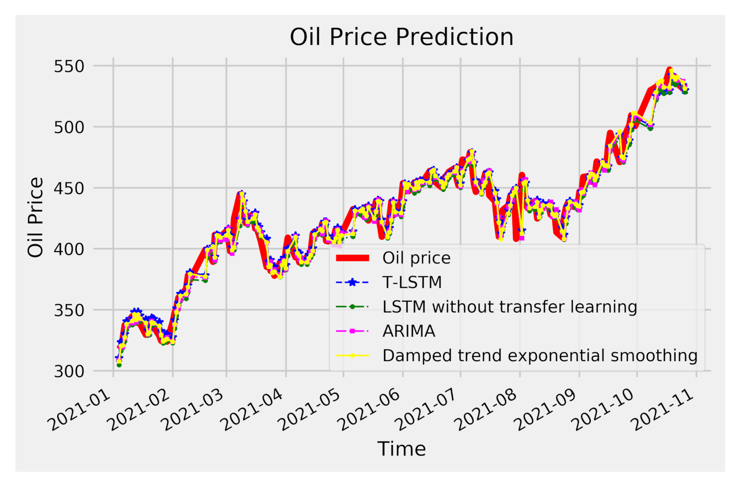
In this section, we compare the experimental result of the proposed transfer learning based LSTM method (T-LSTM) with auto-regressive integrated moving average (ARIMA), damped trend exponential smoothing, and LSTM without transfer learning. All experiments were run on a personal computer with CPU 2.7 GHz and 32 GB RAM. T-LSTM and LSTM were conducted in Python 3.7 via Keras 2.3.1. The neural networks were trained using Adam algorithm with default learning rate 0.001.

We first report the result when the number of neurons of hidden layers n equals 50. We test the T-LSTM and LSTM for different rolling window size {6, 15, 30} and batch size {16, 32, 64}. Here r represents the rolling window size. The Diebold-Mariano (DM) test is applied to determine whether the predictions of T-LSTM and LSTM are significantly different. As we can see from

Table 2. Results for number of neurons of hidden layers $n=50$.

Parameters	Algoritms	RMSE	MAE	MAPE	DAR	p Value of DM Test
r = 6,	T-LSTM	9.84	7.18	1.70	0.51	0.021
batch size = 16	LSTM	10.98	8.29	1.94	0.46
r= 6,	T-LSTM	9.79	7.10	1.67	0.53	0.00014
batch size = 32	LSTM	10.09	7.56	1.77	0.50
r = 6,	T-LSTM	9.91	7.22	1.70	0.50	0.014
batch size = 64	LSTM	10.27	7.65	1.78	0.51
r = 15,	T-LSTM	9.91	7.22	1.69	0.51	0.002
batch size = 16	LSTM	9.92	7.23	1.70	0.51
r = 15,	T-LSTM	9.81	7.12	1.68	0.51	0.013
batch size = 32	LSTM	10.24	7.67	1.81	0.48
r = 15,	T-LSTM	9.82	7.13	1.68	0.53	0.032
batch size = 64	LSTM	10.07	7.53	1.78	0.51
r = 30,	T-LSTM	10.44	7.73	1.81	0.47	0.011
batch size = 16	LSTM	10.23	7.57	1.77	0.48
r = 30,	T-LSTM	9.83	7.11	1.68	0.53	0.103
batch size = 32	LSTM	10.04	7.49	1.77	0.48
r = 30,	T-LSTM	10.01	7.35	1.73	0.53	0.0078
batch size = 64	LSTM	11.19	8.84	2.08	0.50

, for most of the cases, the p value is less than 0.1. It means that the predictions of T-LSTM and LSTM are significantly different. It can be seen from the Table 2 that T-LSTM has smaller predictive error than LSTM in most cases. The proposed T-LSTM obtains the best performance when the rolling window size equals 6 and batch size equals 32.

To do the sensitivity analysis, we compare the results of T-LSTM and LSTM for a number of neurons of hidden layers $n=30$ and $n=100$. As we can see from Table 2, T-LSTM has best performance when the rolling window equals 6. In the following experiment, the rolling window size will be fixed to be 6. The results are shown in

Table 3. Comparison of T-LSTM and LSTM for number of neurons of hidden layers $n=30$ and rolling window size $r=6$.

Parameters	Algoritms	RMSE	MAE	MAPE	DAR	p Value of DM Test
batch size = 16	T-LSTM	10.03	7.35	1.72	0.49	0.0012
	LSTM	11.76	9.18	2.16	0.45
batch size = 32	T-LSTM	9.82	7.16	1.69	0.52	0.054
	LSTM	10.81	8.31	1.95	0.48
batch size = 64	T-LSTM	10.59	8.03	1.88	0.47	0.0040
	LSTM	11.22	8.90	2.10	0.51

and

Table 4. Comparison of T-LSTM and LSTM for a number of neurons of hidden layers $n=100$ and rolling window size $r=6$.

Parameters	Algoritms	RMSE	MAE	MAPE	DAR	p Value of DM Test
batch size = 16	T-LSTM	10.24	7.54	1.76	0.49	0.0353
	LSTM	12.88	10.30	2.39	0.46
batch size = 32	T-LSTM	9.88	7.18	1.69	0.52	0.0182
	LSTM	10.01	7.37	1.73	0.50
batch size = 64	T-LSTM	9.83	7.14	1.68	0.53	0.0316
	LSTM	10.84	8.53	2.01	0.52

for different batch sizes. It can be seen from Table 3 and Table 4 that the transfer learning based method T-LSTM has better performance than LSTM without transfer learning.

In the following, we report the result of ARIMA and damped trend exponential smoothing, which are benchmarks for time series analysis. It can be seen from Figure 4 that the mean of Shanghai crude oil is not stationary, which is also confirmed by the values of the autocorrelation in Figure 6. We can see from Figure 7 that the series of Shanghai crude oil is stationary after first order difference. Figure 8 and Figure 9 shows the autocorrelation and partial differenced Shanghai crude oil price respectively. The ARIMA model used in this paper is the ARIMA(3, 1, 2) which is determined by the auto ARIMA using pmdarima package. For the damped trend exponential smoothing method, the smoothing level is equal to 0.8 and the smoothing slope is equal to 0.2.

The result of the different algorithms are shown in

Table 5. Comparsion of the four methods.

Algoritms	RMSE	MAE	MAPE	DAR
T-LSTM	9.79	7.10	1.67	0.53
LSTM	10.27	7.65	1.78	0.51
ARIMA	10.13	7.31	1.72	0.51
Damped trend exponential smoothing	9.94	7.22	1.70	0.48

. For the T-LSTM and LSTM, the number of neurons of hidden layers n equals 50, the rolling window size equals 6, and batch size equals 32. Note that the results of T-LSTM and LSTM are selected from Table 2 using the same parameters. From the Table 5, it can be seen that the proposed T-LSTM obtains the best performance, which has the smallest RMSE, MAE, and MAPE. The directional accuracy ratio (DAR) of T-LSTM is highest among the four methods.

We also plot the predicted oil prices of four methods in Figure 10. It can be seen that the prediction curve with Brent data is more suitable for the real data curve than the prediction curve with Shanghai data only, which shows that the prediction effect of the model using Brent data for transfer learning is better. With the help of Brent data, the trend of the predicted value and the real value is basically consistent, and the numerical prediction is also similar, and the two curves almost coincide.

4. Conclusions

This paper mainly solves the problem of Shanghai crude oil price prediction. Due to the little accumulation of Shanghai crude oil futures price data, it is difficult to predict. Due to the correlation between Brent crude oil price data and Shanghai crude oil price data, this paper uses transfer learning to predict the Shanghai crude oil price. Through the experiments, it is found that the proposed T-LSTM can accurately predict the crude oil prices of Shanghai, and the model has strong generalization ability and high prediction accuracy.