Abstract
The European Parliament has adopted Directive 2019/1161 on the promotion of environmentally friendly and energy-efficient road transport vehicles, which also defines the obligations and forms of support for the procurement of environmentally friendly vehicles in urban logistics. The increase in the number of shipments delivered within e-commerce, which is also the result of the COVID-19 pandemic, requires a transition to a sustainable logistics system. New research questions are being raised in the preparation of new projects for the introduction of small electric commercial vehicles in particular. One of the main research questions about deployment itself is whether light commercial electric vehicles are able to fully replace conventionally powered vehicles. What operating conditions are optimal for the operation of them? How does load weight affect the energy efficiency of operating a light commercial electric vehicle? The authors decided to carry out research into the impacts of weight and the nature of a driving cycle under laboratory conditions to eliminate all external factors that could distort individual measurements and their results. In order to simulate driving cycles, an urban driving cycle was designed on the basis of the course of speed, acceleration, deceleration and slope conditions of roads in the selected regional city of Žilina (Slovakia). In the case of the operation of an electrically powered light commercial vehicle, the impact of load weight on the range of the vehicle is low, and is below the level of the theoretical maximum range of the vehicle in urban logistics applications. The operation of electrically powered vehicles in hilly terrains with relatively longer gradients and steeper slopes increases electricity consumption and, thereby, reduces their range.
1. Introduction
Transport as a whole is considered to be one of the majority producers of harmful emissions, whether these are gases contributing to the greenhouse effect or substances harmful (not only) to the human body. In the last almost three decades, transport has undergone several changes related to making all transport processes more environmentally friendly. One of the most visible changes is the gradual introduction and tightening of emission limits for internal combustion engines. However, current times show that transport using conventional drives is not permanently sustainable. Permanent sustainability has become a frequently used term in all sectors, not just in transport. In order for all the commitments set out in the strategy documents to be met and the positive effects to be quantified, global cooperation between all stakeholders is essential. However, it is also essential that each entity approaches the greening of its own operations independently and responsibly. Only in this case can a successful system concept that will have a positive effect on its operation be considered. If these ideas are transformed into transport, it is possible to give specific examples. Any environmentally friendly vehicle needs the right mode for its operation. Only in this way is it possible to use its potential and the benefits that its operation should bring. If we talk about so-called green logistics, we must consider the deployment of environmentally friendly vehicles and equipment, in addition to processes involving the ecological elements of logistics chain management. Therefore, it would be possible to clearly identify a connection that is necessary for the successful implementation of realistic greening. It is necessary for each part of the chain, whether it is transport technology or logistics management, to effectively work independently and, at the same time, to arrange for a synergy of their mutual interaction, which can bring results in the form of benefits, especially for the environment.
The European Parliament has adopted Directive 2019/1161 on the promotion of environmentally friendly and energy-efficient road transport vehicles [1], which defines the obligations and forms of support for the procurement of environmentally friendly vehicles, in particular in the urban logistics environment and applications. The directive is transposed into the national legislations of the individual EU member states, with the objective of meeting the set minimum shares for the procurement of environmentally friendly vehicles for road transport in Figure 1.
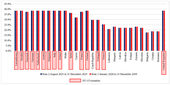
Figure 1.
Minimum target shares for environmentally friendly light commercial clean vehicles (N1) out of the total number of procured N1 vehicles in the EU countries for the 2025 and 2030 horizons. Source: Authors based on [1].
It is, therefore, possible to expect a more rapid development of electromobility in the near future. Electromobility in the field of freight transport is of particular importance. Even though electrification in long-distance transport does not have clear contours yet (apart from overhead trolley-wire motorways and concepts of electric tractors), distribution using electricity as an energy source is already a reality today.
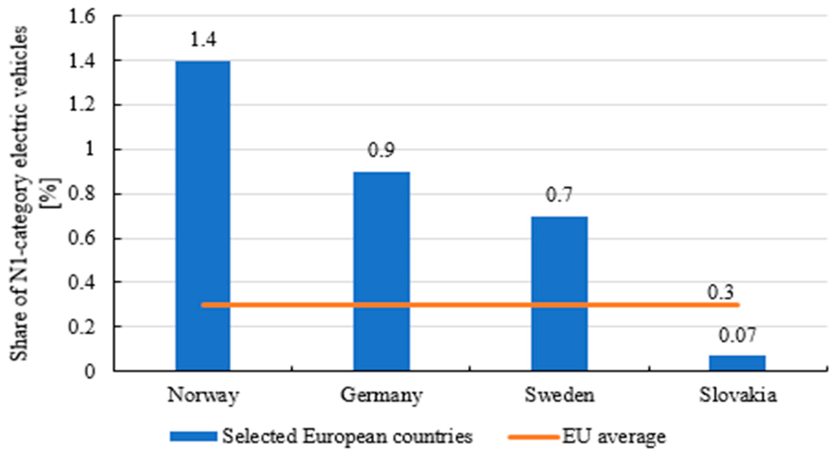
In the Slovak Republic, 269,350 vehicles were registered in the N1 vehicles category as of 22 April 2021. Out of the total number of these vehicles, 182 vehicles, in absolute terms, use electricity as a source of drive. In relative terms, it is possible to state that 0.07% of all vehicles of the given category [2] can be found in the category of N1 light goods vehicles with electric drive in the Slovak Republic. For comparison, it is appropriate to state that, according to ACEA data for 2019, there was a total of 0.3% of electric vehicles in the N1 category in the European Union. Within the EU countries, the largest share of electric light goods vehicles with a total weight of up to 3.5 tons is in Germany (0.9%) and Sweden (0.7%) in Figure 2. However, Norway, which is not subject to the European Union legislative requirements, has the highest share of electric vehicles with a total weight of up to 3.5 tons with the share of these being 1.4% [3].
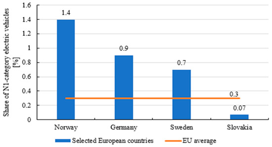
Figure 2.
Share of N1 category: electric vehicles in the EU and selected European countries.
A positive trend in increasing the number of new electric light commercial vehicles in the EU is evident. A comparison of ACEA data between 2019 and 2020 shows that the number of new N1 vehicles in the EU using petrol as fuel was 45.4% lower in 2020, and the number of new diesel vehicles was 17.2% lower. On the contrary, the number of new electric vehicles in the given category was 26.2% higher year by year. Additionally, from the perspective of newly registered vehicles, 2% were electric vehicles up to 3.5 tons and, for instance, the figure reached 8.1% in Norway [4]. It is clear from these data that this trend can be maintained and the share of electric vehicles will continue to increase. Even in the Slovak Republic, up to 51.64% of all N1 vehicles have been registered in the previous years of 2019, 2020 and 2021, and the analysis of historical data shows that the number of newly registered electric commercial vehicles has also been increasing every year in the Slovak Republic.
The use of electromobility in terms of urban logistics is a reality today, albeit a reality that is still being created and formed. There has been the formation of a new technical and technological platform and its application is currently creating a number of research opportunities. It also has issues such as the complexity of its implementation, technological setup, and the subsequent optimization of systems. One of the main questions about implementation itself is whether electric light goods vehicles are able to fully replace conventionally powered vehicles. Under what circumstances is it possible to switch to electric drive? What limitations and opportunities will it bring? What operating conditions are optimal for the operation of electric vehicles? How does load weight affect the energy efficiency of operating such a vehicle? Is an electric vehicle able to operate efficiently in urban distribution?
2. Literature Review
In addition to its benefits, road transport is undoubtedly a source of externalities and it generates external costs, which were compared in inland freight transport in Belgium by Merchan et al. [5]. At the same time, it is necessary to focus on the negative impacts of transport on the environment in city centers [6]. Environmental sustainability is a requirement for modern urban freight transport systems. On a global scale, most resources are currently consumed in cities, and it contributes to the economic importance of urban freight transport as well as to its poor environmental aspects. According to the authors of the study [7], there is a lack of knowledge on how to properly quantify the environmental performance of urban freight transport systems. In this context, Muñoz-Villamizar et al., the authors of the study, propose a methodology for assessing the environmental performance of urban freight transport systems. The authors of the paper [8] state that the level of air pollution stimulates the sale of electric vehicles based on empirical evidence from twenty major Chinese cities. Transport operations are one of the sources of the current pollution problems in urban areas. One of the many reasons for this situation is the growing need for freight transport using different modes of transport, especially road transport. The environmental impact should be one of the more important criteria to be considered when choosing a mode of transport. The objective of Grondys’ contribution [9] was to assess the level of pollution generated from gaseous emissions depending on the vehicle type, category and size of the load, taking into account urban areas. Based on the obtained results, the potential level of pollution in cities was determined and which mode of transport contributes the most to air pollution was found. A similar issue, but in urban public transport, was addressed by Konečný et al. in a paper [10] dealing with the impacts the operation of urban public transport fleets after their modernization had on emissions. In terms of the introduction of environmentally friendly forms of transport while respecting the needs of sustainability, it is necessary to know the specifics of the operation of electric commercial vehicles [11,12]. The environmental effects of electromobility in relation to sustainable urban transport have been investigated by Pietrzak et al. [13]. A similar issue has been addressed by Jereb et al. in a paper [14] examining the impact of traffic flows in urban areas on increasing fuel consumption and on the environment. Researchers at City University of Hong Kong focused on exploring the possibilities of using electric vehicles in areas with traffic congestion. The results show that electric vehicles are able to achieve good results just at times of traffic congestion; when they move at lower speeds, their consumption may be lower, and so it is possible that it is not necessary to charge electric vehicles during distribution in congested traffic. On the other hand, in smooth traffic with higher speeds, these vehicles consume more energy and have to use charging stations during distribution. On the basis of traffic information, it is also possible to anticipate recharging needs, as well as to model the time needed for distribution [15]. The possibility of the wireless charging of electric vehicles while driving through an established system is described in paper [16] that uses a specific example. The method of charging electric vehicles using energy produced from renewable sources was discussed by Małek et al. in their paper [17]. Proper logistical planning is also essential in connection with the knowledge of the specifics of electric vehicle operation, especially in urban applications. Florio et al. provide a relevant methodology in their study for solving the electric vehicle problem on congested street networks [18]. Electric vehicle turnover planning is also addressed in a study by Rubiano et al., who use simulation mathematical-heuristic methods [19]. However, in order to set up individual systems correctly, it is necessary to know the operation of electric vehicles in distribution in the real world. The efficiency of lightweight electric vehicles in last mile deliveries was discussed by Iwan et al. [20] in a paper whose results may be appropriate for transport and logistics companies, and a similar issue was also addressed by the authors in paper [21]. Turner et al. provide a study in which they publish modelling and optimization tools with emission quantification in the supply and service of the food retailing industry [22]. The impact of the full electrification of the vehicle fleet providing postal services for urban environments has been examined by Martínez et al. [23]. A similar issue is addressed through a case study from Rio de Janeiro by de Mello Bandeira et al. [24]. A comparison of light commercial vehicles using diesel and electricity in city logistics from an economic and environmental point of view was made in a paper by Giordano et al. [25] and Melo et al. [26]. A cost comparison for lightweight commercial vehicles with alternative and conventional drives was also performed by Scorrano et al. [27]. Various policy measures [28] and the integration of electric vehicles into light commercial vehicle logistics operations [29,30] may help to increase the use of electric vehicles in cities. The introduction of electric vehicles for distribution in urban freight transport is currently a significant opportunity to improve urban environments [31]. The political priorities of some countries are to reduce the harmful effects of road transport on the environment and health and to reduce the number of road accidents. Various technologies could improve air quality, and reduce energy consumption and CO2 emissions from road vehicles. A remarkable research issue in the transition from internal combustion vehicles to alternative technologies is to understand how intelligent transport systems and other transport-related measures can contribute to a reduction in fuel consumption and greenhouse gas emissions [32]. Mikusova et al. deal with the technological and economic context of renewable and non-renewable electricity in electromobility in Slovakia and Hungary [33].
In connection with the logistics planning for electric vehicles, the development of the network of charging stations in the area and the possibilities of charging vehicles [34,35] is one of the important factors. In their paper, Csizár et al. [36] dealt with the development of a methodology for determining suitable places for the construction of charging stations for electric vehicles. The connection between the optimization of logistics planning and vehicle charging is also in the implementation of intelligent infrastructure elements. Schau et al. investigated the contribution of smart infrastructure elements to the development of electromobility in distribution services in a smart city logistics environment [37]. Taniguchi et al. also studied the increase in the efficiency of urban logistics using innovative technologies. The paper presents the ways in which the correct use of modelling and planning can contribute to an overall increase in the efficiency and competitiveness of urban logistics [38]. Kretzschmar et al. presented range prediction models that are based on machine learning and take into account a wide range of input parameters, such as weather, traffic level, and topographic data. The presented models have their application in the environment of urban logistics [39]. In addition to external parameters and external planning factors, it is necessary to take into consideration the specifics of the vehicles themselves. In terms of innovative systems, care must be taken to ensure that electric vehicles in operation are equipped with a suitable battery management system [40,41]. One of the important parameters that need to be taken into account when purchasing vehicles is the size and capacity of the traction battery [42]. In freight transport environments, it is mainly a balance between the required range and the payload of vehicles.
Topographic data and the data on traffic density and speed in the studied area are an important part of modelling and planning. For the correct calibration and setting of logistics planning, it is necessary to thoroughly know the electric light commercial vehicles’ operational efficiency in individual operating modes. A study by Tong and Ng from Hong Kong [43], which examines bus driving cycles, focuses on differences in driving cycles, especially in relation to cost effectiveness. A similar research approach needs to be applied in freight transport, and the data can be used not only to assess the cost effectiveness and to control the amount of emissions produced, but also for sound logistics management. A study by Komorovska et al. presented the results of studies of simulated driving cycles and the performance of the algorithm when applied to real recorded driving cycles of an electric vehicle [44]. Possibilities of using a traction system consisting of a battery and a superconductor to increase the range based on processing topographic data on road gradients is dealt with in a paper by Hu et al. [45].
The efficiency of the deployment of electric vehicles is important mainly within the last mile, where it can be combined with the use of electric freight bicycles [46] and the establishment of urban logistics or consolidation centers [47].
3. Materials and Methods
The authors decided to carry out research into the impacts of weight and the nature of a driving cycle in isolated, laboratory conditions. The authors chose this method to eliminate all external factors that could distort individual measurements and their results. There was a risk that the resulting impact of weight measured would be distorted by the effect of changing outdoor temperatures, differences in traffic in individual measurements, and wind direction and speed, etc. The aim was to find out the exact, isolated impact of the load weight on the range, as well as the impact of the nature of a driving cycle. Measurements were performed at the MAHA MSR 1050 vehicle dynamometer with the possibility of simulating various driving cycles.
Due to the fact that the outside temperature can fundamentally affect the range of the vehicle and the efficiency of the battery, we performed the measurements in an indoor manner at laboratory temperatures within the range of 19–22 °C. During the measurements, all additional electrical equipment and comfort equipment in the vehicle (heating, air conditioning, seat and steering wheel heating, radio, etc.) were switched off. The daylight mode of the headlights was switched on during the measurements. Halogen bulbs stored in the front fog lamps of the measured vehicle were used as daytime running lights.
The Nissan Voltia electric commercial vehicle with the following characteristics of the basic parameters was chosen for the measurements:
- A 3-phase synchronous electric motor with an output of 80 kW and a torque of 254 Nm;
- A traction battery with a capacity of 40 kWh;
- A single-speed gearbox with a P, R, N, D mode controller;
- An operating weight according to the registration certificate (1677 kg); and
- A maximum permissible total weight according to the registration certificate (2220 kg).
For the purpose of the measurements under laboratory conditions to simulate the operation of the electric vehicle, it was necessary to determine the driving resistances of the vehicle for the correct course of the measurements. Due to the fact that the measurements were based on a mutual comparison of the measured values (between the empty and loaded vehicle and between the individual driving cycles), it was possible to use reference values of driving resistance for a small van.
Driving resistances that the vehicle’s motor must overcome include rolling resistance, drag, inertia and road grade resistance.
Rolling resistance is the resistance arising from the deformation of a tire, a pad under a tire, or a combination of both. The value of the rolling resistance is given by:
- Fr is the rolling resistance (N);
- m is the vehicle weight (kg);
- g is the gravitational constant (m·s−2); and
- f is the rolling resistance coefficient (RRC/1000) (-) [48].
As follows from Equation (1), rolling resistance is present whenever a vehicle is moving and always acts against the vehicle’s direction of travel.
Drag depends mainly on the driving speed and the shape and dimensions of a vehicle and can be expressed by:
- Fa is drag (N);
- v is driving speed (m·s−1);
- A is the size of the frontal area of the vehicle (m2);
- cd is drag coefficient, expressing the aerodynamic shape of the vehicle (-); and
- ρ is air density (kg·m−3) [49].
Together with rolling resistance, drag is always present when the vehicle is moving and also always acts against the vehicle’s direction of travel.
Another driving resistance is inertia, which always acts when the vehicle is not moving at a constant speed:
- Fac is inertia (N);
- m is the vehicle weight (kg);
- a is the acceleration of the vehicle (m·s−2); and
- σ is the coefficient of resistance of rotating masses to changes in rotational speed (-) [50].
Road grade resistance depends on the weight of the vehicle and the angle of the slope of the road to the horizontal plane, and its value is given by:
- Fc is grade resistance (N);
- m is the vehicle weight (kg);
- g is the gravitational constant (m·s−2); and
- α is the angle of the road to the horizontal plane (°) [51].
The analysis of Equations (1)–(4) shows that rolling resistance and drag always act against the direction of the travel of the vehicle, whereas inertia and road grade resistance can act both in the direction and against the direction of the travel of the vehicle. The analysis of Equations (1)–(4) also shows that a change in vehicle weight causes an increase in the rolling resistance value, grade resistance, and inertia, but as mentioned in the previous part of the article, an increase in inertia and an increase in grade resistance may not always also mean an increased energy consumption of the vehicle’s motor, as they can also act in the direction of travel. This may be reflected in the impact of vehicle weight on the energy performance of a vehicle, in particular when the vehicle has the feature of recovering the kinetic energy of the vehicle into electricity, as is the case with the vehicle used for the measurements.
For the purposes of the performed measurements, it was necessary to prepare driving cycles for the whole simulation. The crucial element was a modified urban driving cycle for the city of Žilina based on the course of speed, acceleration, and deceleration in traffic in the city of Žilina. At the same time, it contained a projected vertical profile of the route, which reflects the profile of roads in the city of Žilina. The profile was formed by flat to slightly rolling terrain with several short sections of steeper (up to 12%) downhill and uphill routings. In the measurements, a cycle was approximately 9 km long. The driving cycle was created through real measurements in traffic in the city of Žilina.
For the design of routes, it was first necessary to determine the central geo-points of the individual city districts. The central geo-point is the point at which it is assumed that all roads assigned to one zone (part) have their beginning and end at this one center of the district. Its position may or may not always be the geometric center of a zone. When defining the position of the central geo-point, it was necessary to consider the number and position of a building in a given area. The following Table 1 provides an overview of the individual routes and basic information about the routes such as start point, end point, length and number of inhabitants served.

Table 1.
Overview of individual routes and their basic information.
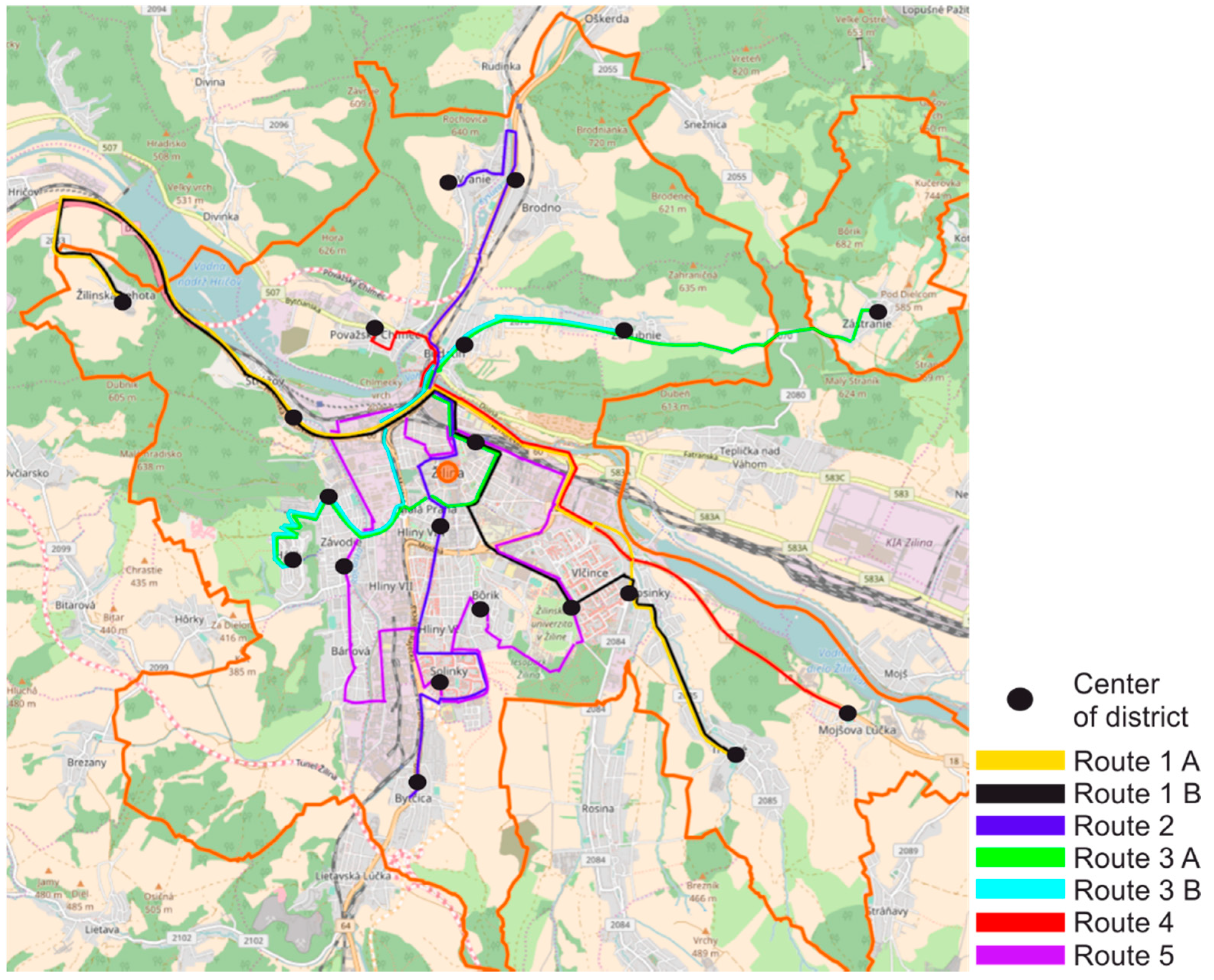
It is possible to see a graphical representation of the individual routes shown on the map in Figure 3. As can be seen, the proposed routes represent a dense road network and create interconnections between city districts. Figure 3 shows the central geo-points of the individual city districts through which the proposed routes lead.
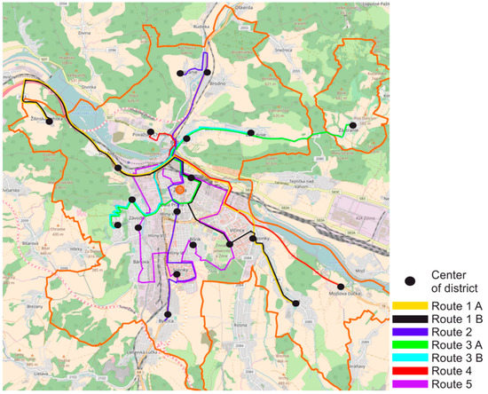
Figure 3.
Map of the city of Žilina with the individual routes marked. Source: Authors.
The measurements and data collection were performed with the Volkswagen Golf 1.9 TDI along the proposed routes. Data collection was performed and recorded in both directions of the routes and the measurements were performed twice on a given route, for the transport peak and the transport trough. A peak is expected to have a higher intensity of vehicles in road traffic and also a peak depends on the given situation in road traffic. There are two peaks during a day.
A driving cycle is a dependence of speed on time and it consists of stopping, constant speed, acceleration, and deceleration. A developed driving cycle is determined by the driving pattern of the given traffic in the operation of the vehicle.
Based on the selected parameters of the weighted arithmetic mean and their values, the proposed methodology represents a developed, simplified and smoothed driving cycle for the city of Žilina. This driving cycle is not based on real data and may not show the actual operation of the vehicle in urban traffic. In this case, it is a polygonal driving cycle.
Design of a Simulation Driving Cycle Based on Selected Parameters of the Weighted Arithmetic Mean
When determining the resulting cycle, the authors used selected parameters of the weighted arithmetic mean. The times of the following parameters were taken into account to design this cycle:
- Total time;
- Driving time;
- Idling time;
- Constant speed;
- Acceleration time;
- Deceleration time;
- Intervals of individual speeds; and
- Number of stops.
The number of stops is the basic parameter that is selected to design a cycle. Based on the weighted arithmetic mean, the number of stops is 11.56, i.e., 12 stops. The resulting cycle will represent 12 stops with the total stop length determined by the weighted arithmetic mean of 118.29 s. These stops are evenly distributed and the length of one is 9.86 s. A cycle will also contain 12 simplified runs separated by this idling time.
Furthermore, it is based on the intervals of individual speeds determined by the weighted arithmetic mean. Speed intervals of 0–15 km/h, 15.1–30 km/h, 30.1–50 km/h, 50.1–70 km/h, and 70.1–90 km/h are considered.
Speeds of 30.1–55 km/h are included in the interval of 30.1–50 km/h, due to the fact that when measuring on the routes, the speed of 50 km/h could have been exceeded. In the interval 50.1–70 km/h, the speeds from 55.1–75 km/h are included in the interval as well, again due to possible speeding on the expressway leading through the city, where the speed limit is 70 km/h. All speeds higher than 75 km/h are included in the range of 70.1–90 km/h. The duration of the individual speed intervals will be divided by the number of stops, with the interval of 50.1–70 km/h occurring twice in the total cycle and the interval of 70.1–90 km/h occurring once, given that these intervals contain a short time and that it would, in fact, not be possible to achieve this division between the 12 parts. Other important parameters for cycle design are constant speed times, acceleration times, and deceleration times. It is necessary to determine their percentage from these times, where 100% is the sum of these times.
Since the resulting cycle will be smoothed, simplification is used by multiplying the interval time by the percentage of constant speed time, acceleration time and deceleration time. Constant speed is assigned to the highest value of the interval, namely 15 km/h, 30 km/h, 50 km/h, 70 km/h and 90 km/h. The times of these speeds are different and are shown in the following Table 2, which also shows the acceleration and deceleration times within individual intervals, the total time in a given interval, and the time of one section for a given interval.
Table 2.
Table of times for individual intervals for designing the final cycle.
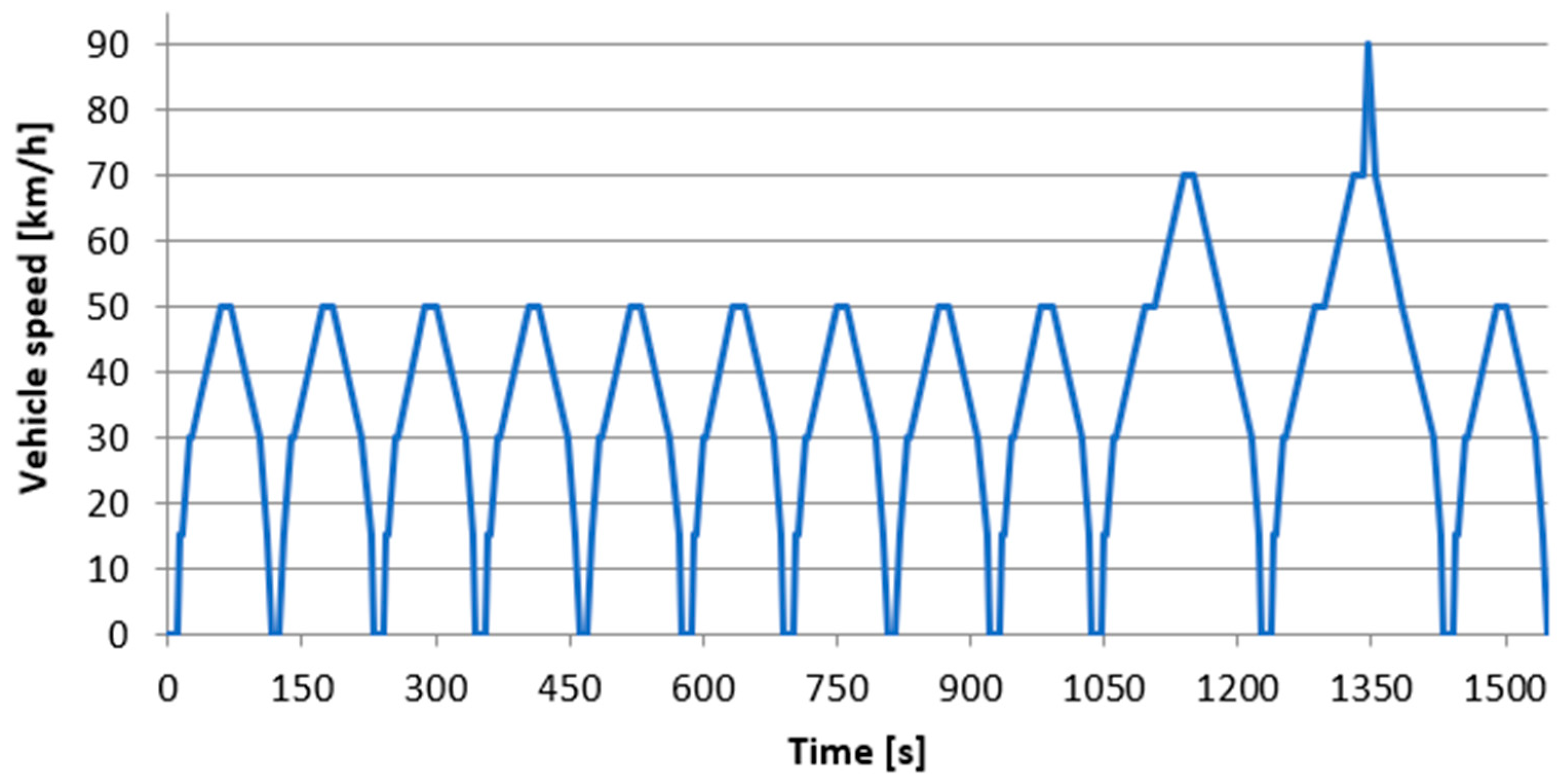
Based on this table, it is possible to compile a graph that represents the resulting driving cycle designed from selected values of the weighted arithmetic mean in Figure 4.
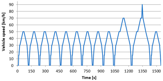
Figure 4.
Resulting driving cycle.
The resulting cycle time is the same as in the weighted arithmetic mean and is 1546 s. The values of the average speed, the maximum speed and the total distance driven are not the same as in the weighted arithmetic mean due to the fact that the simplified values of the weighted arithmetic mean were used. The distance driven during the cycle is 15,226.04 m. The maximum cycle speed is 90 km/h and the average speed is 35.43 km/h. In the following figure it is possible to see the course of speed up to 50 km/h.
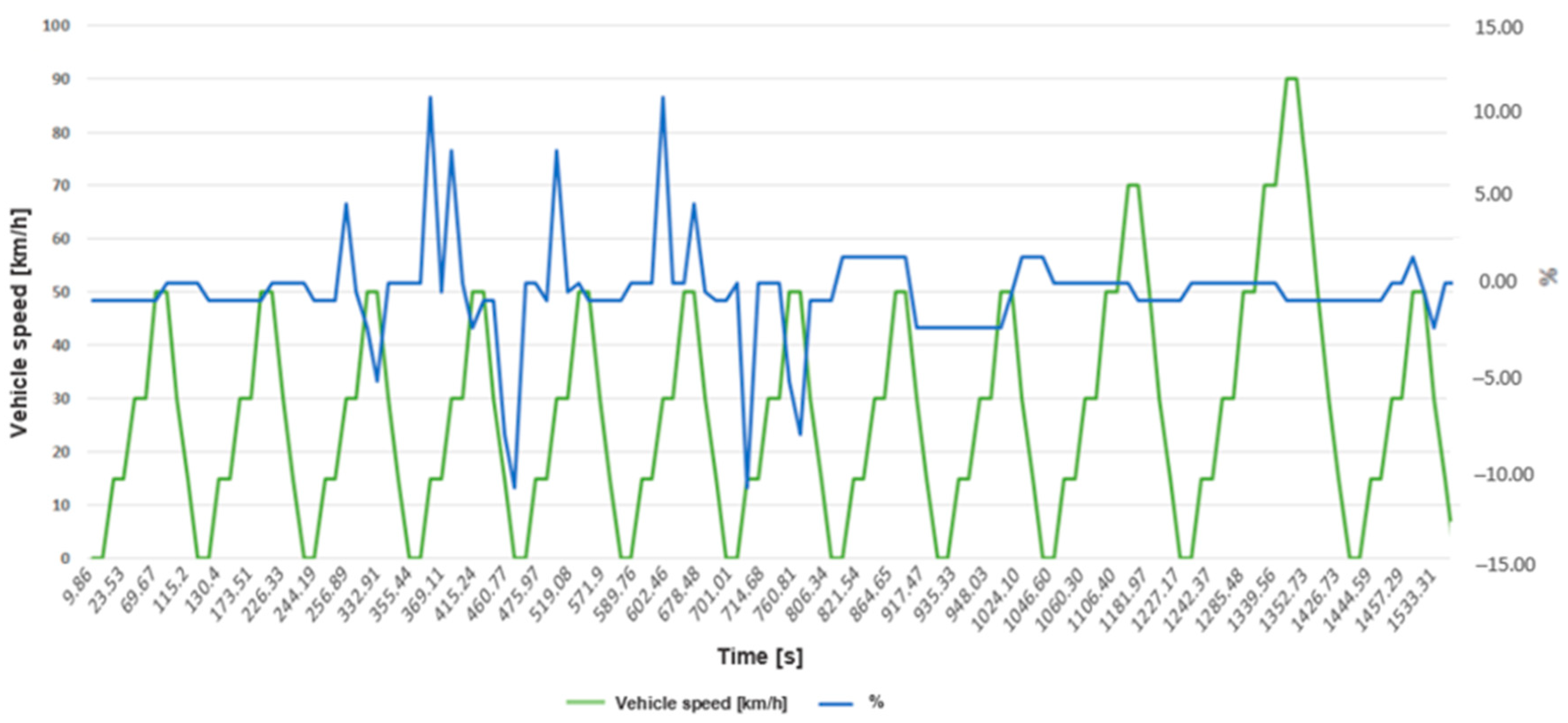
The entire driving cycle contains a total of 12 segments and, therefore, the effort was to apply the expressed percentages from vertical profile measurement intervals as accurately as possible in accordance with the distances specified in tables for the distribution of cycle parts. As a result, we tried to divide the intervals so that they correspond to the shape of the five studied routes while respecting the weights of the individual routes based on the number of inhabitants living in the served urban districts. The graphical application of the entire division of the vertical profile into the driving cycle is shown in Figure 5.
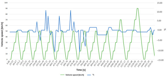
Figure 5.
Application of the vertical profile to a driving cycle.
The maximum vertical profile interval for an uphill section that was applied was 11%. The maximum interval of the vertical profile application for a downhill section was at the level of 11%.
By modifying the basic urban cycle, the authors simulated various other operating conditions. The first modification was designing the entire driving cycle to an uphill gradient of 4%. In this case, it is not primarily about the simulations of real operating conditions, but about the simulations of a situation where the impact of recuperation, i.e., energy recovery through deceleration and downhill driving, is limited. The objective was to compare the decrease in battery charge level when driving in the basic urban cycle, where the conditions were created for a significant share of energy recovery as compared to the driving cycle where there would be a minimum share for energy recovery.
By further modifying the vertical profile of the basic urban driving cycle, the authors obtained a fragmented profile with longer and steeper uphill phases as well as downhill phases as compared to the basic cycle. In the first half of the modified driving cycle, there were continuously long uphill phases with a slope of 4–12%, followed by downhill phases with an analogous slope in the middle of the driving cycle. The end of the cycle was conducted in a flat and very mild terrain profile. The objective of the modification was to compare the driving behaviour of the vehicle within one driving cycle when driving on relatively steep and long uphill gradients as compared to driving in flat or slightly rolling terrain. At the same time, the authors also monitored the impact of downhill gradients on the vehicle’s powertrain control.
All the mentioned driving cycles, which were created by modifying the basic urban driving cycle, had a length of about 9 km in the measurements.
As part of studying the impact of the higher constant speed, the authors created a driving cycle of approximately 25 km in length, which included sections with a constant speed of 50 km/h, several decelerations and accelerations within the range of 30–50 km/h, and one short stop. The cycle profile was driven with several shorter and longer uphill and downhill phases within the slope range of up to 12%. The objective of the driving cycle was to investigate the impact of a higher speed on the decrease in the battery charge level or electricity consumption.
The authors then combined all the driving cycles into certain series and blocks during the measurements. They compiled five blocks of driving cycles and applied them to the empty and loaded vehicle in the same order of the series of driving cycles.
- (1)
- Series of basic city cycles: four basic urban driving cycles were included in a row within the first block;
- (2)
- Urban driving cycle in a constant slope of 4%, without the subsequent repetition of the driving cycle within the block;
- (3)
- Urban driving cycle with fragmented terrain with a slope of 4–12%, without repeating the driving cycle within the block;
- (4)
- Series of driving cycles at a constant speed of 30–50 km/h. Two identical successive driving cycles were included within the block; and
- (5)
- Series of different driving cycles. A series of individual driving cycles was included in the last block:
- Basic urban cycle (once);
- Urban driving cycle with fragmented terrain 4–12% (once); and
- Driving cycle at a constant speed of 30–50 km/h (once).
4. Results
4.1. Impact of Vehicle Load on Its Range
When investigating the impact of load on the vehicle’s range, the authors proceeded from the general assumption that the vehicle load will have a significant impact on the range of the electric vehicle; that is, as the vehicle load increases, the vehicle’s battery will discharge faster.
The authors performed the measurements of a series of various driving cycles, recording the battery charge level after each cycle. The authors completed the whole series of cycles in the same order and under the same conditions with the simulation of the vehicle when empty and fully loaded, whereas the vehicle dynamometer was simulating the respective driving resistances depending on the size of the vehicle load. The authors drove 147 km with the vehicle when empty as well as loaded. The operating weight of the vehicle according to the vehicle registration certificate was 1677 kg, and the total weight was 2220 kg. The authors proceeded from the mentioned values according to the certificate of registration. The difference, i.e., the payload, is 543 kg, and it is 32.4% (approximately 1/3) of the curb weight.
In Figure 6, it is possible to follow the graphical course of the decrease in the charge level of the vehicle’s traction battery during the individual driving cycles. It can be concluded that if the battery reached more than 50% of its charge level, there was no significant difference between the consumption of the vehicle when empty or loaded. The differences in the individual checkpoints after completing the respective driving cycles either showed no differences or only slight differences in the battery charge at the level of 1–2%.
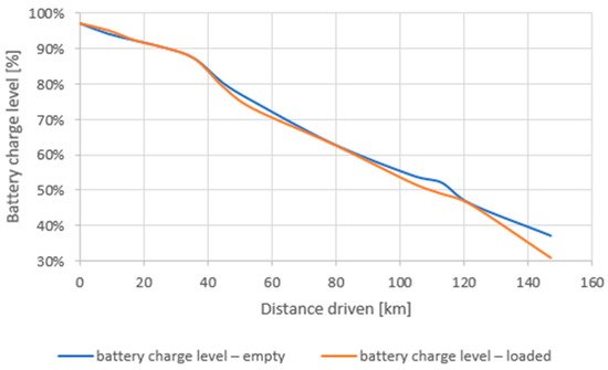
Figure 6.
Comparison of the decrease in battery charge level during driving cycle simulations with empty and loaded vehicles.
A more significant difference does not begin to manifest itself until the battery charge level drops below 50%. After completing the whole series of driving cycles, i.e., 147 km, the residual battery charge level was 37% when the vehicle was empty (1677 kg), and the battery reached a final residual charge level of 31% when the vehicle was fully loaded. The difference in battery charge level is 6%. Depending on the terrain in which the electrically powered vehicle will move, the difference of 6% in battery charge level represents a range of approximately 15–20 km.
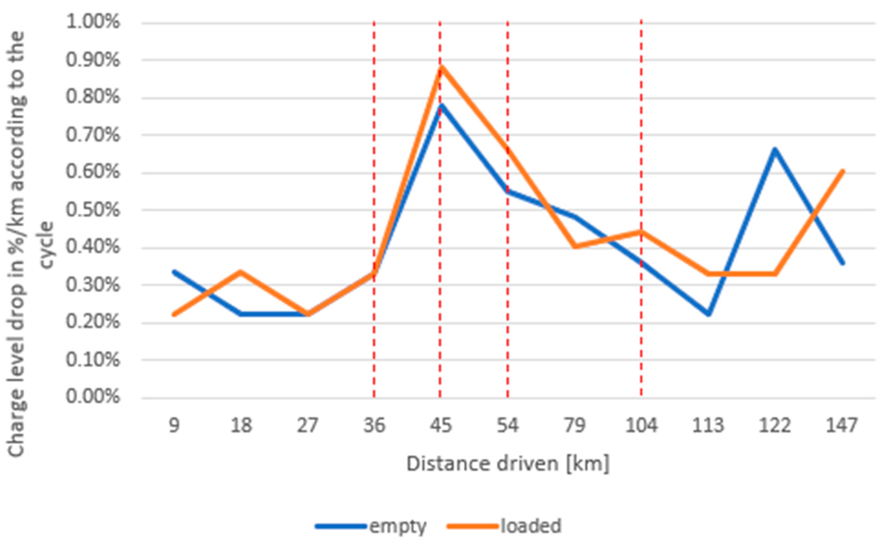
Figure 7 shows the decrease in the battery charge level, expressed as a percentage of the decrease per 1 km of distance driven in the individual driving cycles as compared to the vehicle when it is empty and loaded. It can be identified according to the graphical course that the curve of the loaded vehicle’s relative discharging of the battery is, for the most part, slightly above the curve that plots the course for the empty vehicle. In some cases, the curves are identical and in some cases the curve of the loaded vehicle is even below the curve of the empty vehicle. The average relative decrease in the battery charge level when the vehicle is empty reaches the level of 0.41%, and when the vehicle is loaded, it reaches a slightly higher level, namely 0.43%. It can be concluded from the above two graphical comparisons that the weight of the load has a certain, but small (in the case of the examined vehicle category) impact on the range of the vehicle. At the same time, however, it should be noted that for vehicles of higher categories or as the payload/vehicle’s operating weight ratio increases, the difference in energy consumption between empty and loaded vehicles may increase. This characteristic applies only to vehicles with a lower payload/operating weight ratio which, in principle, applied only to small light commercial vehicles. Note: the red dashed lines separate the individual blocks of the driving cycles.
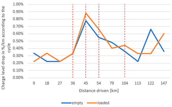
Figure 7.
Decrease in battery charge level during driving cycles expressed in %/km.
Additionally, it can be concluded from the graphical course in Figure 8 that although the decrease in charge level in relation to the weight of the load does not reach a high level, it is clear that when the battery charge level drops below 50%, it discharges faster, especially when the vehicle is loaded. This is documented in particular by the last measured driving cycle, where there is a significant difference in the decrease in battery charge level between empty and loaded vehicles.
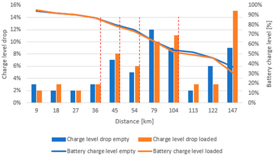
Figure 8.
The course of the decrease in the battery charge level when the vehicle is empty and loaded with the expression of partial relative decreases.
It is also necessary to add to the conclusion that the electric vehicle has a high degree of recuperation, i.e., the reverse flow of energy during braking or after releasing the accelerator pedal. Due to the fact that the loaded vehicle reaches a higher value of kinetic energy, which needs to be wasted during deceleration, there is also a higher rate of recovery, and the vehicle’s traction battery can be recharged more with this recovered energy than in the case of the empty vehicle with lower kinetic energy.
4.2. Impact of Driving Cycle Character on Operational Efficiency
Just as there are relatively significant differences in energy consumption for vehicles with an internal combustion engine depending on the nature of driving and the terrain, for electrically powered vehicles, there are also differences in energy consumption and, therefore, in operating efficiency depending on the type of terrain in which such vehicles are operated. In terms of formulating the principles of the methodology in relation to the procurement of electrically powered vehicles, which are to replace conventionally powered vehicles, it is necessary to know the specifics of electrically powered vehicles perfectly in order to maximize their potential and to take advantage of their operational benefits.
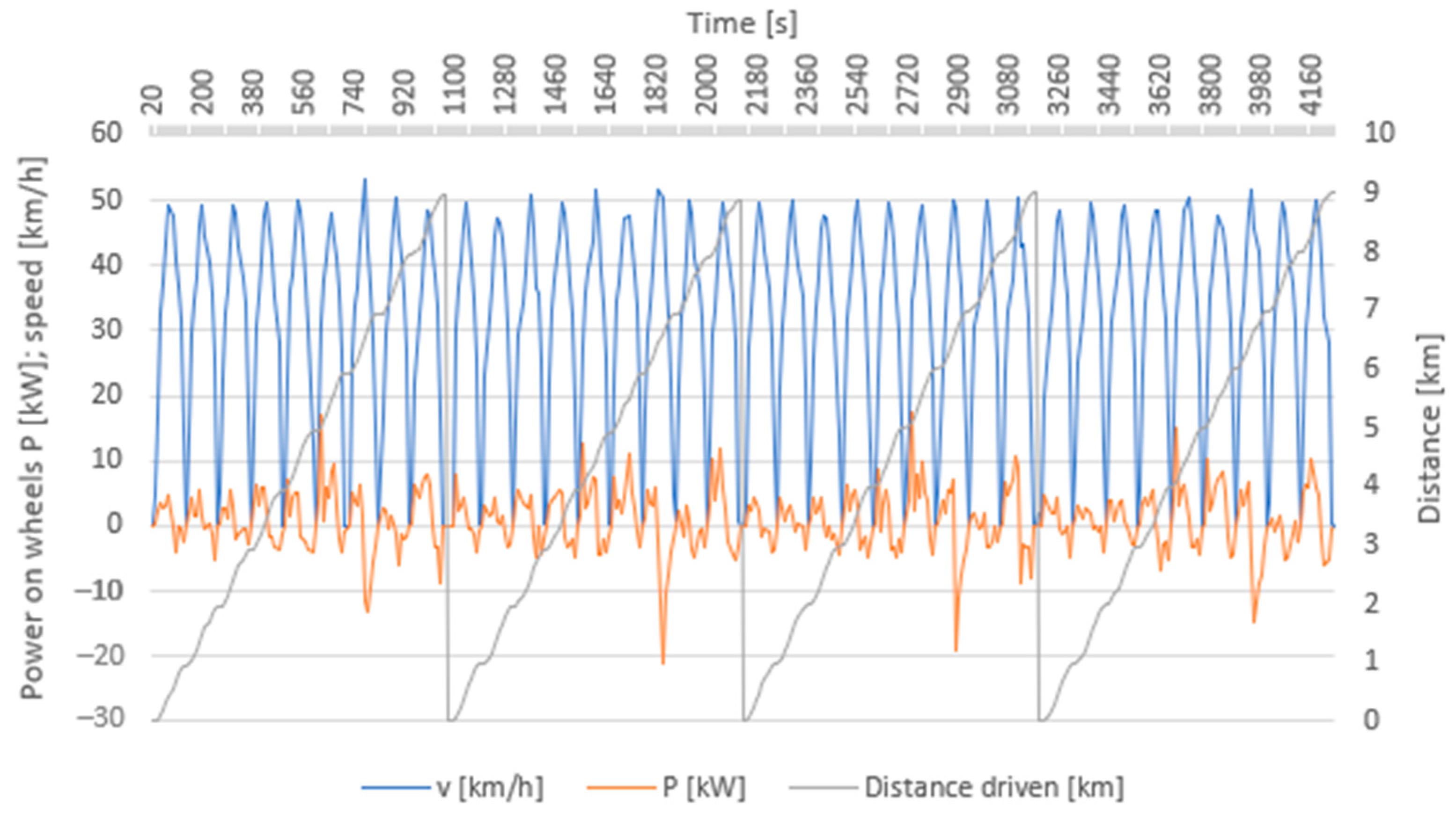
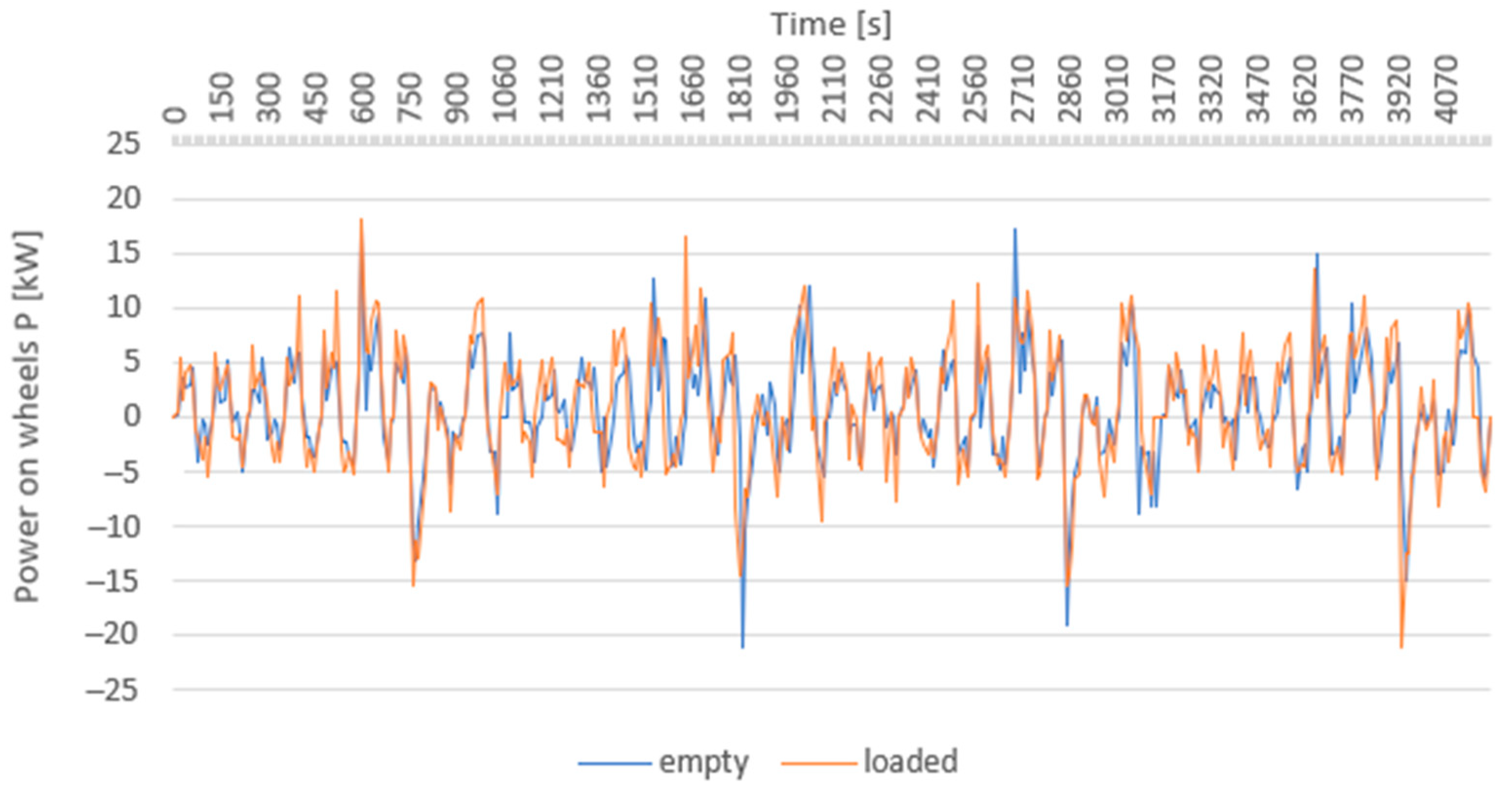
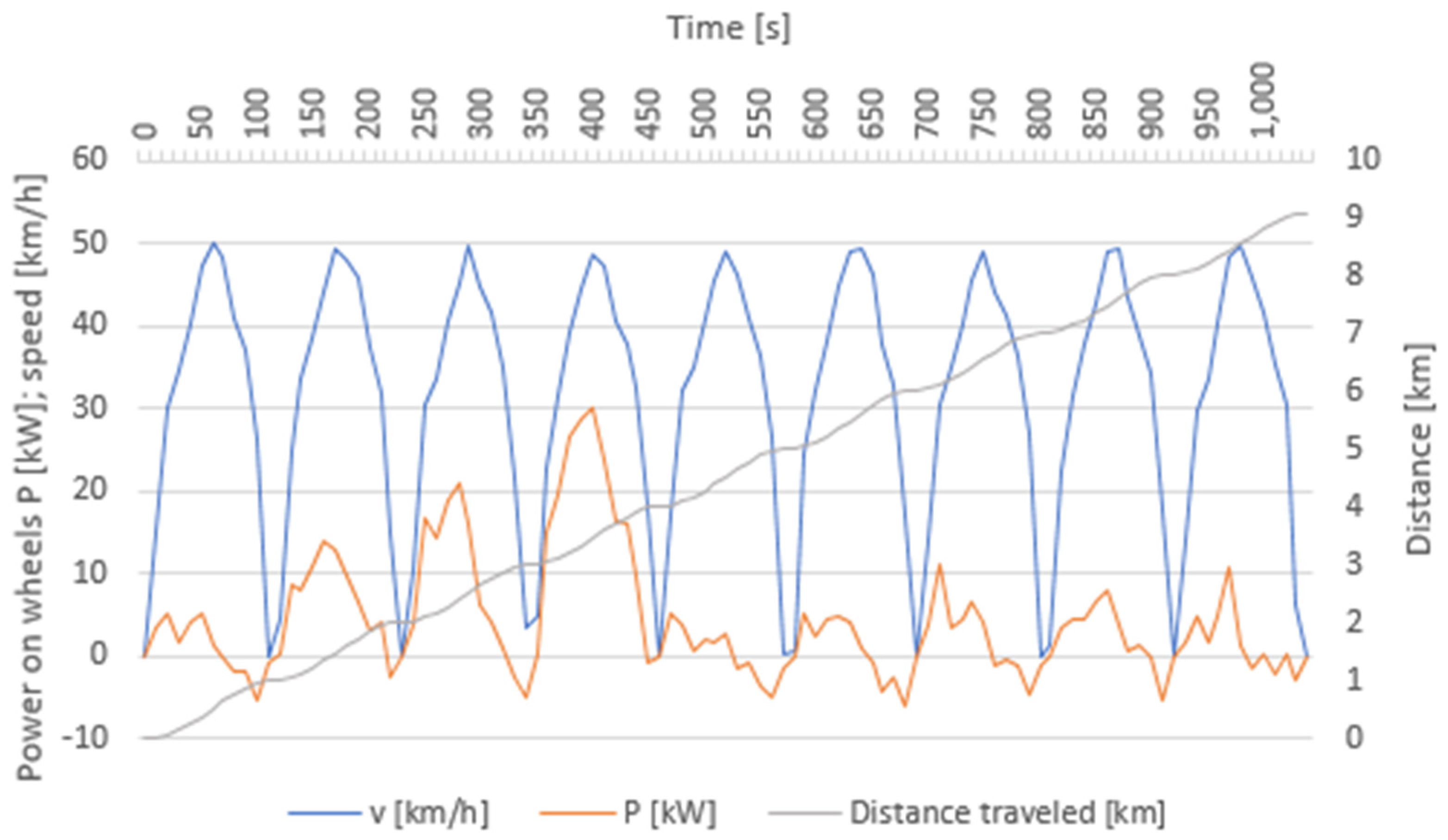
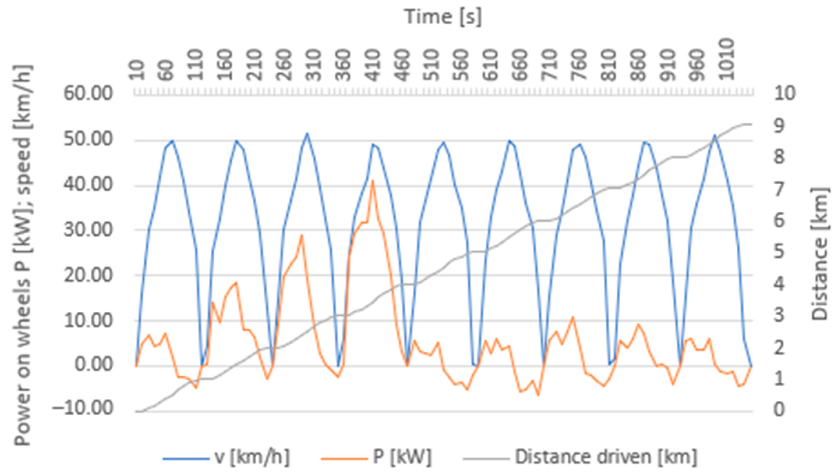
As part of a series of test driving cycles, the first series of four basic urban cycles (same in succession) contains mostly flat terrain with short uphill gradients, including moving off to drive uphill. In order to distinguish the individual driving cycles from each other, the distance driven in Figure 9 and Figure 10 starts from zero for each new driving cycle. It can be clearly identified from the graphic course in Figure 11, which contains a comparison of the performance of the power on wheels, that a large part of the performance extends to the negative axis; that is, driving in an urban cycle is very advantageous for an electrically powered vehicle as there are many opportunities for recuperation, i.e., recharging the battery, which contributes to low battery discharge. It can also be seen that the power on wheels is low for most of the driving time, which also contributes to low battery discharge.

Figure 9.
Record of selected values for a series of four basic urban cycles (empty vehicle).
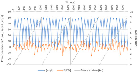
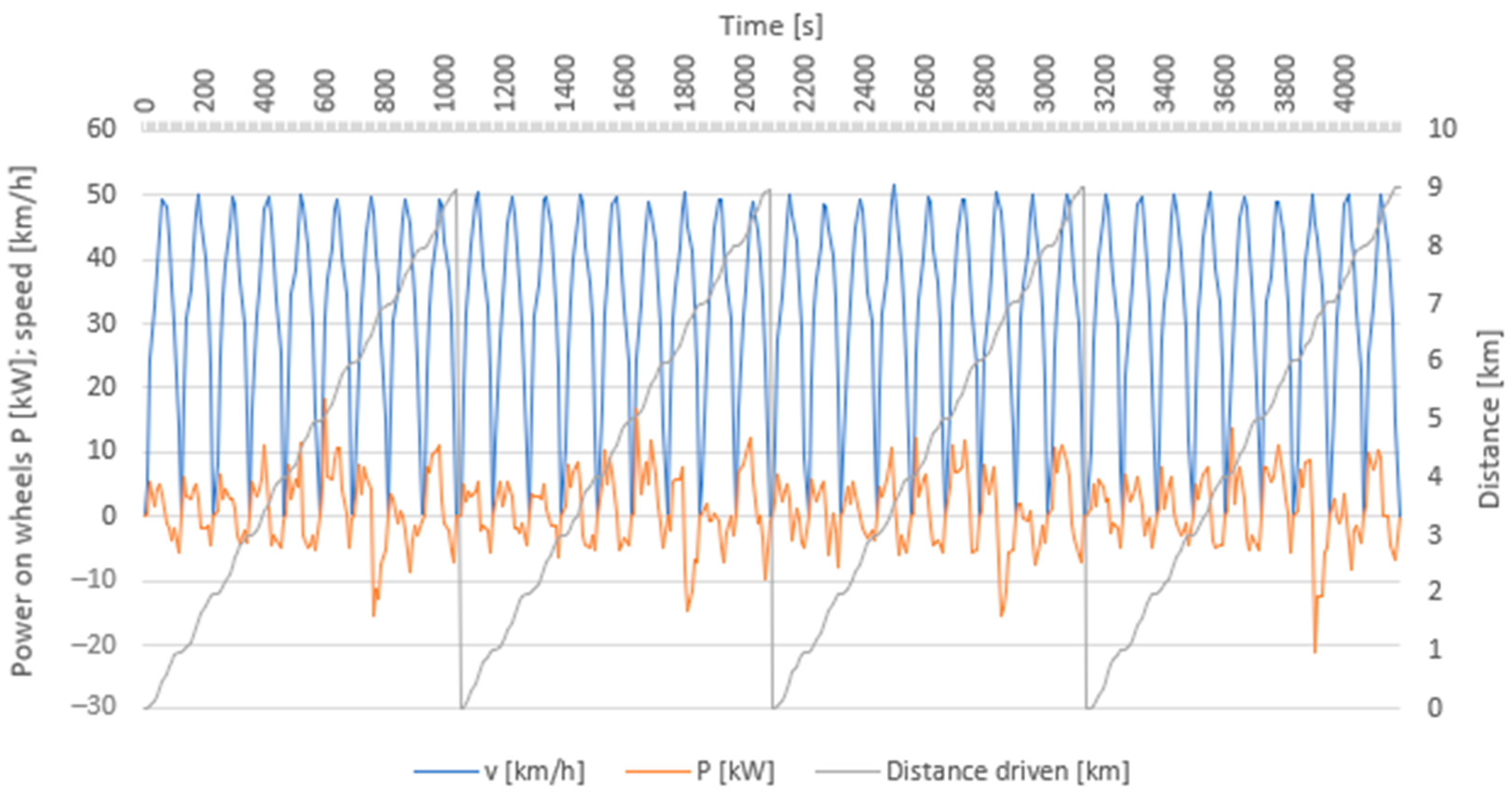
Figure 10.
Record of selected values for a series of four basic urban cycles (loaded vehicle).
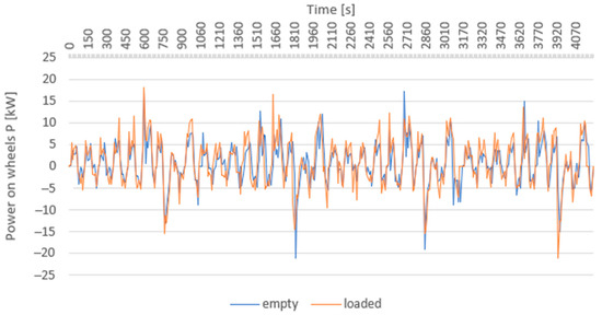
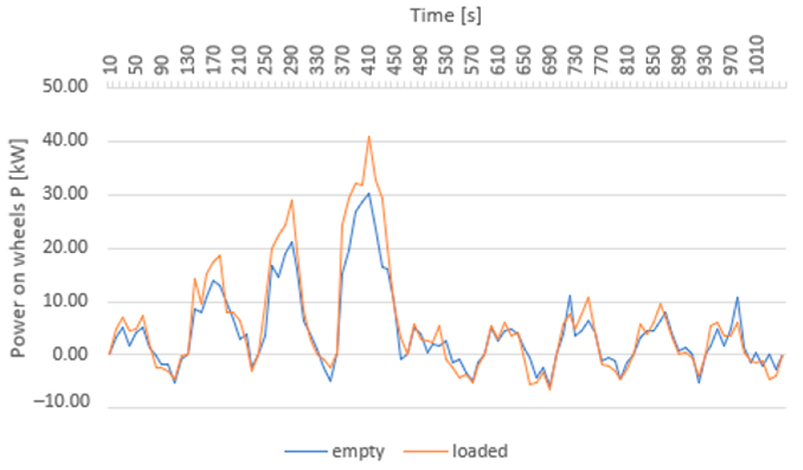
Figure 11.
Comparison of the power on wheels in a series of four basic urban cycles with the vehicle being empty and loaded.
Another important parameter is the fact that the curves of empty and loaded vehicles are almost identical and there are no significant differences between them, except for some short-term peak values. This means that the vehicle can operate in an urban environment very efficiently with low electricity consumption, regardless of the loading level.
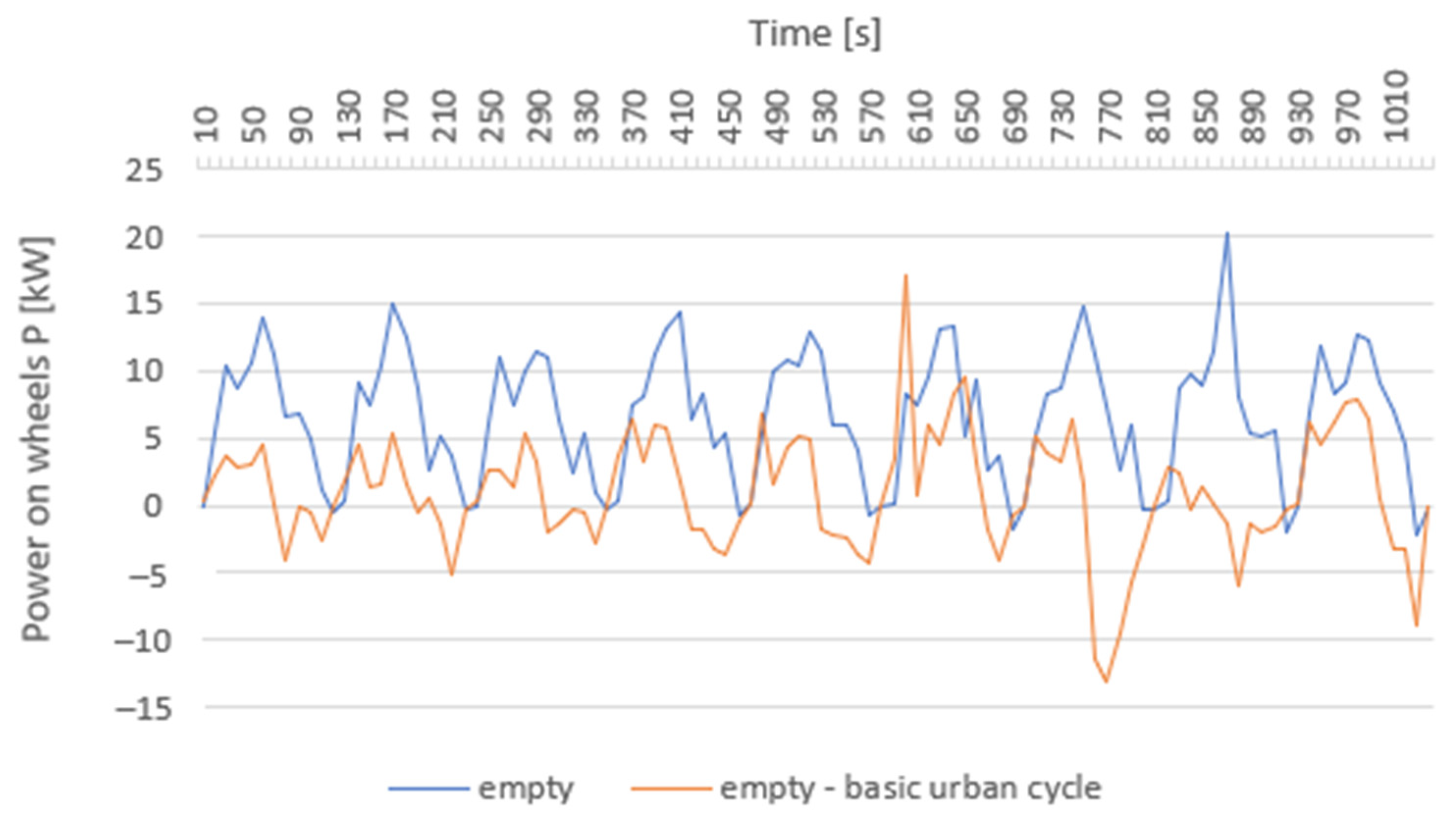
When the speed profile of the basic urban driving cycle was modified by placing it at a constant 4% uphill gradient, there was a significant difference in the required power on wheels, which is shown in Figure 12. The graphic course demonstrates the difference in the power on wheels of an empty vehicle in the basic urban cycle (burgundy curve) and in the cycle with a constant 4% uphill rising (blue curve). Apart from a significant increase in the power on wheels when driving in 4% uphill gradients, almost no opportunities for energy recovery can be observed in the same speed profile. When driving in the basic urban driving cycle, the relative decrease in the battery charge level after completing one cycle reached 2–3%. When driving in 4% uphill gradients in the same speed profile, the relative loss in battery charge level reached up to 7%, i.e., more than twice as much. It can be stated that when driving uphill, electric drive is energy-intensive and electricity consumption increases significantly.
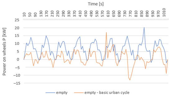
Figure 12.
Comparison of wheel performance with an empty vehicle in the basic urban driving cycle and in the urban driving cycle in 4% uphill gradients.
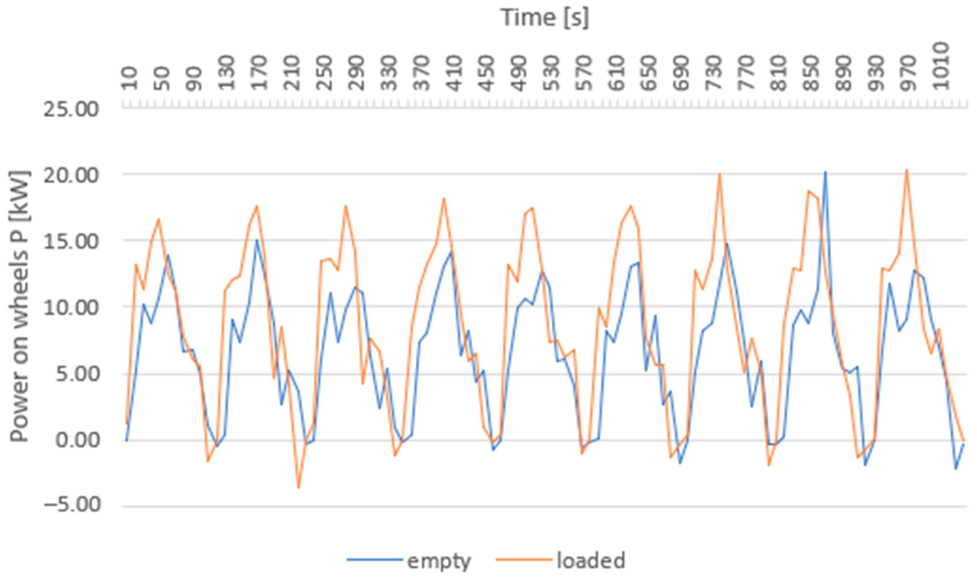
When comparing the power on wheels in the driving cycle simulation with a 4% uphill rising, it is possible to identify in Figure 13 a noticeable difference between an empty and a loaded vehicle. In the case of comparing an empty and a loaded vehicle in the basic urban driving cycle, no significant differences were observable at all, with the exception of some peak values. In the case under examination, however, the difference in the power on wheels is noticeable practically throughout a driving cycle. This confirms the assumption that electric drive is less efficient in terrains with gradients than in urban environments with flat and rolling terrain. The relative decrease in battery charge level was 7% per cycle when driving with an empty vehicle. When driving with a loaded vehicle, the decrease was at the level of 8%. However, it should be noted that the simulations were performed at a high battery level (above 80%) and, based on the measurement results, it can be assumed that at a lower overall battery level (below 50%), the difference between an empty and a loaded vehicle could widen.
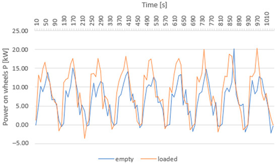
Figure 13.
Comparison of the power wheels in an urban driving cycle in a 4% uphill gradient when the vehicle is empty and loaded.
A driving cycle with steep uphill gradients consisted of longer, more gradual risings with a slope of 4–12% in the first half of the driving cycle, followed by downhill gradients with the same slope from the middle of the driving cycle, and the last third of the driving cycle was in flat or very mildly rolling terrain. It can be seen in the graphic course of the performance on the wheels for the first half of the driving cycle that there was practically no significant opportunity for recuperation, as it was an uphill drive. At the same time, it is possible to formulate that with a empty vehicle (Figure 14) as well as an loaded vehicle (Figure 15), there is a higher power on wheels, which also requires higher electricity consumption. It is possible to identify from the comparison between loaded and empty vehicles in Figure 16 a noticeable increase in the power on wheels in the case of the loaded vehicle and driving uphill, which suggests that there is a difference between loaded and empty vehicles in hilly terrains.
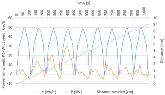
Figure 14.
Record of selected values during a driving cycle with steep uphill gradients (empty vehicle).
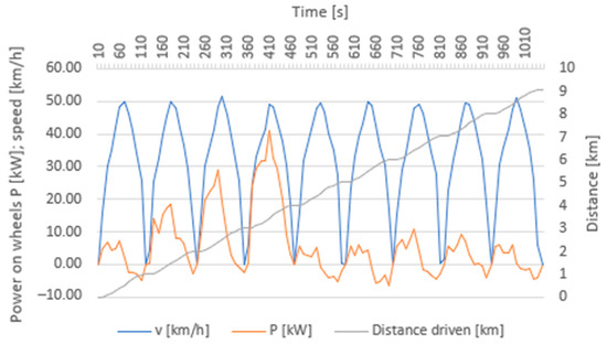
Figure 15.
Record of selected values during a driving cycle with steep uphill gradients (loaded vehicle).

Figure 16.
Comparison of the power on wheels in a driving cycle with a steep uphill gradient when the vehicle is empty and loaded.
When driving downhill, only a minimum power on wheels in the middle of the driving cycle and a certain degree of recuperation expressed in terms of negative power on wheels were recorded in the graphical course. In the last third of the driving cycle, which took place on flat terrain or only in very mild terrain, it is possible to identify again, as in the basic urban cycles, almost identical courses for a loaded and an empty vehicle.
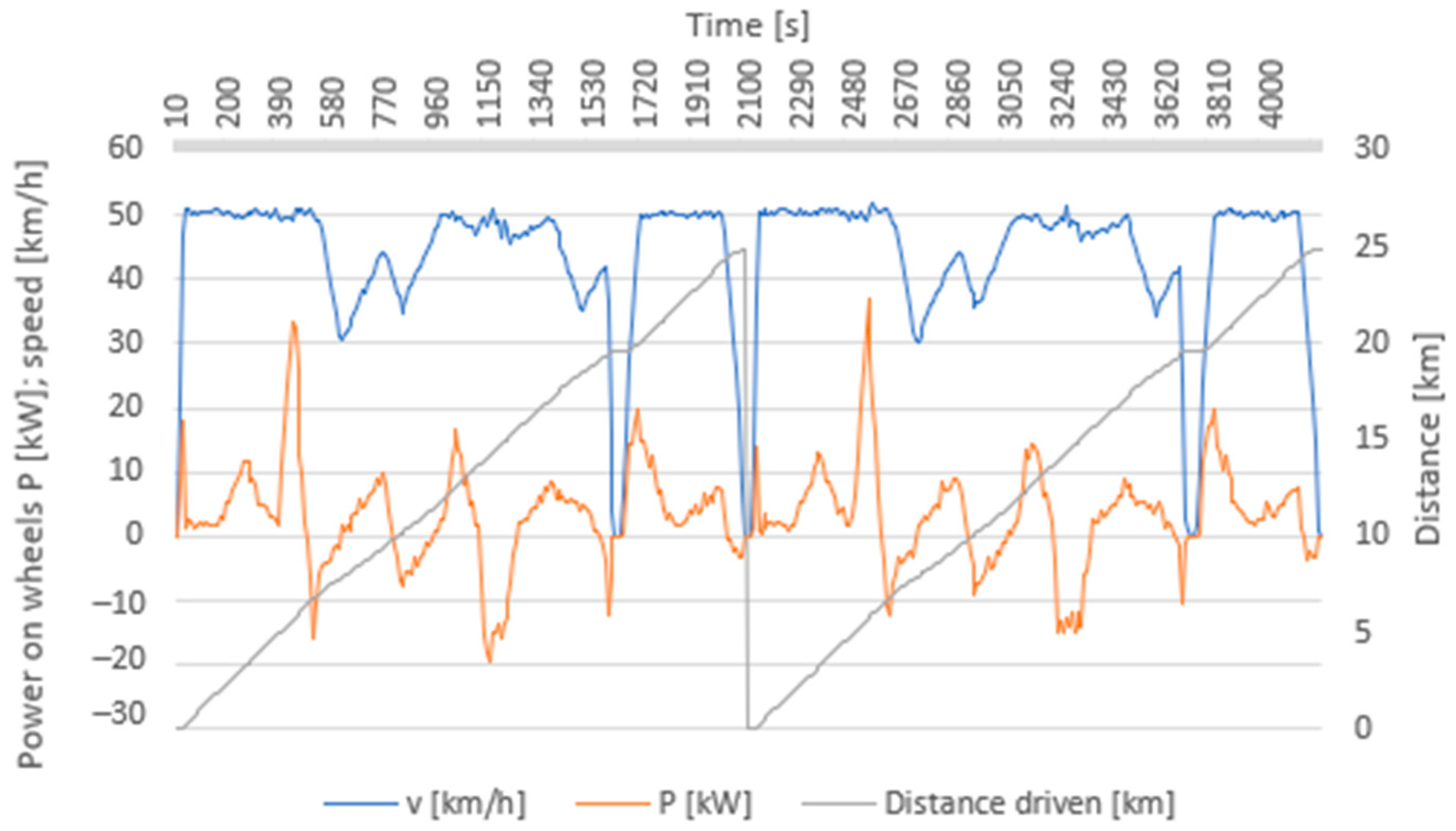
A driving cycle that recorded driving at the constant speeds, most often 50 km/h with several decelerations and accelerations, was also included in the series of driving cycles. The driving cycle was placed in a mixed profile, which contained continuously slight (2–4%) uphill gradients, steep (12%) uphill gradients, analogous downhill gradients, and also flat sections. The main objective was to study the impact of higher speeds (but still oriented towards urban traffic) on the efficiency of the operation of an electric light commercial vehicle. It should be noted that operating at a higher constant speed means higher power consumption and a faster decrease in the battery charge level. However, the electric vehicle itself was able to work efficiently even in these conditions. As can be seen from the graphical curves for the power on wheels, there were plenty of opportunities for energy recovery during the driving cycles, which means a positive compensation for higher energy consumption when driving at higher speeds. The recovery rate depends on the kinetic energy of a vehicle, which is higher at higher vehicle speeds (vehicle speed has an exponential effect on the kinetic energy, whereas weight is only linear) and thus, the recovery rate may be higher. From the point of view of the recuperation rate, the profile in which a vehicle moves, as well as the nature of traffic, is decisive. If the driving profile contains sufficient downhill phases, sufficient space is created for vehicle recuperation, and if the nature of traffic requires the regular slow deceleration of a vehicle and subsequent (not abrupt) moving off, operating the vehicle at higher speeds has a positive impact on its energy efficiency. Of course, the rate and efficiency of recuperation do not depend only on external conditions, such as terrain profile or traffic density and intensity. The design and setting of the vehicle’s driveline also have an effect. When the accelerator control is released, the electric vehicle usually does not “sail” but decelerates significantly. This is due to the activation of energy return, which seeks to efficiently use the vehicle’s kinetic energy and convert it into electrical energy. The return flow of energy causes a significant braking effect on the vehicle (compared to a conventionally powered vehicle, there is a much lower need to use the service brake). In a driving style where the driver uses a regenerative deceleration of the vehicle (instead of a sharp deceleration and a sharp start), it is possible to positively influence the BEV range.
There is evaluated the power on wheels of the investigated vehicles in the empty (Figure 17) and loaded (Figure 18) operation. The mutual comparison of their curve courses are introduced for their higher informative value in the Figure 19.
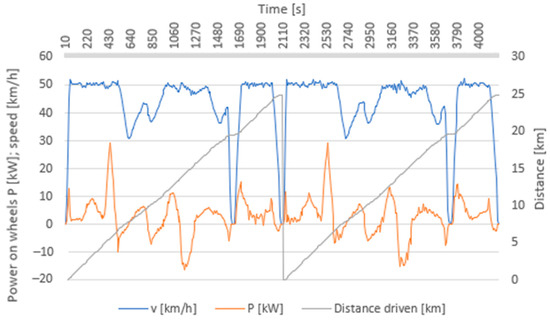
Figure 17.
Series of two driving cycles within the speed range of 30–50 km/h in a mixed profile (empty vehicle).
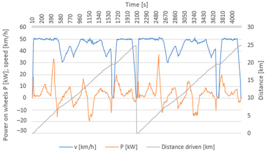
Figure 18.
Series of two driving cycles within the speed range of 30–50 km/h in a mixed profile (loaded vehicle).
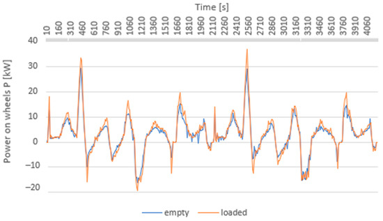
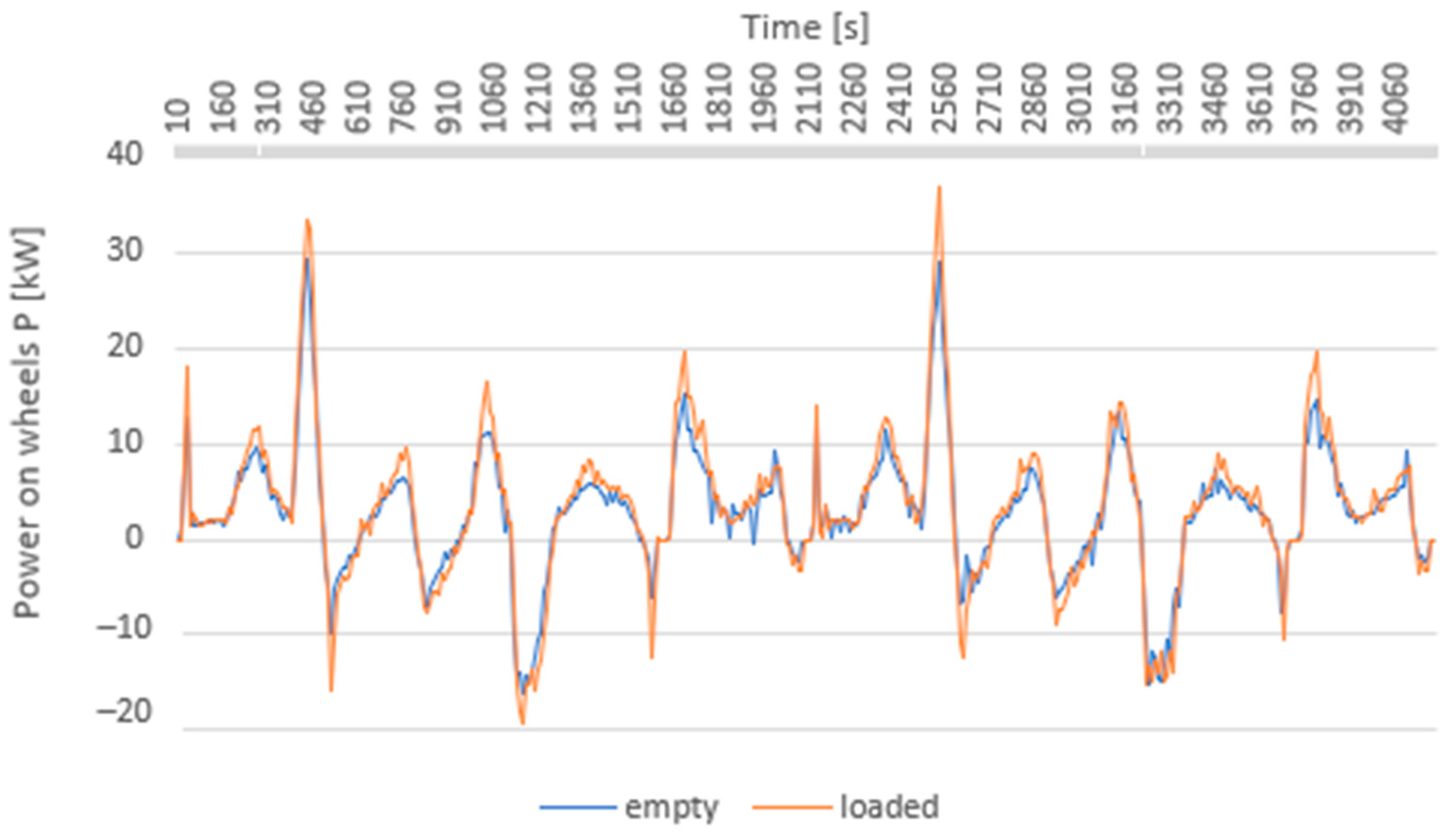
Figure 19.
Comparison of the power on wheels in a series of two driving cycles within the speed range of 30–50 km/h for an empty and loaded vehicle.
A comparison of the power on wheels for a loaded and empty vehicle makes it possible to state that even in the case of the driving cycle in question, there are no significant differences between an empty vehicle and a loaded vehicle.
Differences were recorded only in certain peak values for a very short time. Peak values were reached only in cases where there were steeper uphill phases. The same effect was manifested in downhill phases, where there are some differences in vehicle deceleration, when more force is needed to slow down or stop a loaded vehicle, which is further reflected in higher, negative power on wheels, especially in peak values. This effect creates room for a higher rate of recuperation, i.e., energy recovery. However, as is clear from the graphic course, this does not have a major impact in this specific examined driving cycle.
5. Discussion
In the case of the operation of an electrically powered light commercial vehicle, or a vehicle with a relatively low payload, the impact of load weight on the range of the vehicle is low (well below the level of the theoretical maximum range of the vehicle) in urban logistics applications.
For these reasons, it is essential that electric vehicles are to be operated in as much of an urban environment as possible to maximize the positive effects of such an operation. This can be achieved if urban logistics centers are set up in an optimal allocation to customers [52,53].
At present, mainly multinational logistics companies are putting electric vans into operation in urban logistics as part of their own projects for various customers. At the same time, the effectiveness of the deployment and possible shortcomings are identified only on the basis of their deployment in real operations. Therefore, future research directions could be focused on the compilation of urban cycles according to the specific cities surveyed and the subsequent publication of recommendations for the deployment of light commercial electric vehicles. The efficiency of the deployment of these vehicles also increases with the increase in the cost of fossil fuels and AdBlue, the technical complexity of exhaust gas cleaning systems with which vehicles must be equipped (EGR, DPF, SCR), and also with the increase in support incentives for the procurement and operation of electric vehicles. Further research is possible here. Some research results have been published in [27]. When comparing calculations of electric vehicle emissions against the operation of diesel vehicles in particular, it is also necessary to consider the emissions of these vehicles operating specifically in urban environments with emissions from the forced regeneration of particulate filters, which often needs to be performed outside normal vehicle operation, i.e., after decommissioning these vehicles or when they are in service centers. On the other hand, it must be considered that the production of NOx emissions in the urban operation of diesel engines of ordinary passenger cars that meet the Euro 6 emission limits is 5 to 16 times lower than the declared production according to the measuring cycles; in addition, we must also consider the production of CO2, which is about 94% higher than its value declared by vehicle manufacturers [54]. At the same time, indirect and external emissions from electric vehicles need to be taken into account as well.
The economic aspect of operating electric but conventional vehicles is also an incentive for the continuation of research activities. In general, with increasing pressure to move towards a green economy, the prices of energy, such as fossil fuels and fossil products, are rising and so are the prices of electricity, which have room for further increases due to a rising demand for electric vehicles (which also causes an increase in electricity consumption). However, there are currently problems with the availability of additional reducing agents (AdBlue), which are essential for the proper operation of diesel vehicles. In connection with the increasing price and decreasing availability of reducing agents, there is a presumption of an increase in the number of unauthorized interventions in the emission systems of diesel vehicles, which may cause the operation of vehicles that do not properly control nitrogen (NOx) emissions.
The results of the research published in the paper do not take into account the impact of changes in outdoor temperature on electricity consumption (winter and summer operation), the impact of drivers’ driving techniques, etc. The impetus for further discussions is seen in the issue of the winter operation of electrically powered vehicles (BEV), where there are significant differences in energy consumption as compared to operation at optimal temperature conditions [55]. The differences are mainly caused by the need to heat the vehicle, or steering wheel heating and seat heating, which significantly increases electricity consumption and causes a rapid reduction in the capacity of a vehicle battery, with low temperatures alone reducing battery capacity and operating efficiency [56]. These problems can be resolved with electric vehicle heating systems during charging, where the driver/operator/fleet operator sets the exact time at which a vehicle is to be heated. During charging, it is possible to use waste heat generated during charging. After completion, it is possible to use energy from the electrical grid to which a vehicle is connected during standstill. This ensures the optimum interior temperature of the vehicle upon the first daily start, which partially reduces the energy consumption of the vehicle during operation; that is, the energy stored in the vehicle battery is saved. At the same time, it is possible to keep the vehicle battery at the optimum temperature, thus ensuring efficient use of its capacity even at lower outdoor temperatures. The test vehicle used in this research was equipped with a similar heating system. Nevertheless, in different seasons with significant changes in outdoor temperature (summer and winter), it is possible to expect deviations against the results obtained.
Significant topics in the field of charging efficiency, such as energy that is actually used to charge electric vehicles and the subsequent possibilities to refine the calculation of CO2 emissions of vehicles, have been addressed by Tansini et al. [57]. The importance of the correct use of alternative propulsion vehicles in order to maximize the positive effects of reducing emissions is also highlighted by a study comparing the change in the determination of produced emissions between NEDC and WLTP [58]. Similarly, this research paper emphasizes the correct application of electric vehicles and the importance of logistics and process planning. Similarly, the authors of the research in [59], who carried out the measurements in real driving conditions, state that the biggest positive differences in emissions production between the operation of conventionally and electrically powered electric vehicles occur in urban environments. As the results of our measurements show, much of the efficiency lies in regenerating energy while reducing a vehicle’s speed. Kullingsjö and Karlsson address the importance of this issue in relation to the efficient use of energy obtained, arguing that the share of energy at the wheels used for braking was found to range from 12% to 63%, with an average of 30%. Engine braking could, however, reduce the amount of recoverable energy to about 16% [60].
Research projects on the deployment of autonomous electric light commercial vehicles in urban logistics [61] also need to examine the impacts of changes in outdoor temperature, airflow and road vertical profile in a specific environment where they are to be deployed.
The authors also recommend involving the public in promoting new innovative urban logistics projects so that citizens understand the importance of road freight transport for the functioning of cities, as stated by Amaya, J. et al. in [62].
6. Conclusions
It is possible to state the following conclusions based on the measured values and their evaluation, but also on the basis of experience and observations during the measurements:
- The weight of a load has a measurable impact on light commercial vehicles, which, however, does not represent a significant limitation on the range of BEV in the operating conditions of urban logistics.
- An electric vehicle can operate very efficiently in terms of energy consumption in urban cycles with frequent stops and when it starts at low (urban) speeds. For example, no emissions are generated when delivering consignments to customers as part of courier services.
- For profiles with longer and steeper uphill gradients, the operating efficiency of electrically powered vehicles decreases significantly, and the difference in energy consumption between empty and loaded vehicles also begins to show significantly, where loaded vehicles need significantly more energy to move uphill than empty vehicles. Therefore, electric vehicles are more suitable for places without major uphill routings. When planning the distribution routes, it is necessary to add the percentage slope of uphill and downhill gradients on specific sections of roads to optimization algorithms.
- The difference in drops in battery charge levels between empty and loaded vehicles becomes more pronounced at lower battery charge levels. For longer delivery routes, it is also useful to introduce recharging during unloading in order to achieve recharging above a certain level (e.g., above 50%).
In terms of the impact of driving cycles on vehicle range, the authors have clearly identified that operating at low speeds in urban environments is highly efficient for electrically powered vehicles. Operation in hilly terrain with relatively longer uphill phases with steeper slopes, increases electricity consumption and, thereby, reduces the range of electrically powered electric vehicles. At the same time, when driving in hilly terrain, the difference between the consumption of empty and loaded vehicles deepens. When driving at higher constant speeds, the consumption of electricity also increases more significantly, which has a negative effect on vehicle range but there are also no significant differences between empty and loaded vehicles. The advantages of electrically powered light commercial vehicles will be used in cities with frequent congestion, in cities with reduced maximum driving speeds, e.g., zones with speed limits of 30 km/h (e.g., Paris from 30 July 2021), etc.
The COVID-19 pandemic has significantly increased the demand for e-commerce and there has been an associated increase in consignments in urban logistics. This requires changes in logistics solutions, such as urban logistics centers, but it creates opportunities for the greater use of lightweight electric vehicles. The design and implementation of projects must be based on the conditions of a particular city; in this case, it was the regional city of Žilina, which had 81,953 inhabitants as of 30 September 2021, and a specific light commercial electric vehicle, Nissan Voltia, which, in this case, had a payload of 580 kg. The deployment of electric light goods vehicles is a crucial element of new logistics projects for the sustainability of urban logistics.
Author Contributions
Introduction, J.G., M.D. and T.S. (Tomáš Settey); literature review, J.G., M.D., T.S. (Tomáš Skrúcaný), F.S. and T.S. (Tomáš Settey); materials and methods, J.G., M.D., T.S. (Tomáš Skrúcaný), F.S. and T.S. (Tomáš Settey); data curation, J.G., M.D., T.S. (Tomáš Skrúcaný), F.S. and T.S. (Tomáš Settey); results, J.G., M.D., T.S. (Tomáš Skrúcaný), F.S. and T.S. (Tomáš Settey); writing—original draft, J.G., M.D., T.S. (Tomáš Skrúcaný) and T.S. (Tomáš Settey); visualization, J.G., M.D., T.S. (Tomáš Skrúcaný), F.S. and T.S. (Tomáš Settey). All authors have read and agreed to the published version of the manuscript.
Funding
This research was facilitated by the support under the Operational Program Integrated Infrastructure for the following project: Identification and possibilities of the implementation of new technological measures in transport to achieve safe mobility during a pandemic caused by COVID-19 (ITMS code: 313011AUX5), co-financed by the European Regional Development Fund.
Institutional Review Board Statement
Not applicable.
Informed Consent Statement
Not applicable.
Conflicts of Interest
The authors declare no conflict of interest.
References
- Directive (EU) 2019/1161 of the European Parliament and of the Council of 20 June 2019 Amending Directive 2009/33/EC on the Promotion of Clean and Energy-Efficient Road Transport Vehicles. Available online: https://eur-lex.europa.eu/legal-content/EN/TXT/PDF/?uri=CELEX:32019L1161&qid=1610109503291&from=SK (accessed on 23 September 2021).
- Ministry of Interior of the Slovak Republic. Central Register of Vehicles of the Slovak Republic. Available online: https://www.minv.sk/?celkovy-pocet-evidovanych-vozidiel-v-sr (accessed on 23 September 2021).
- ACEA Report. Vehicles in Use Europe. January 2021. Available online: https://www.acea.auto/uploads/publications/report-vehicles-in-use-europe-january-2021.pdf?fbclid=IwAR2rql7XQPGbJ7DgWZwlppBnuQlrJCkeFgvGPrSl7Z5vVwSKdq0Icd9gUOo (accessed on 23 September 2021).
- ACEA. Light Commercial Vehicles (Up to 3.5t) New Registrations by Fuel Type in the European Union. Full—Year 2020. 19 March 2021. Available online: https://www.acea.auto/files/ACEA_vans_by_fuel_type_full-year_2020.pdf (accessed on 23 September 2021).
- Merchan, A.L.; Léonard, A.; Limbourg, S.; Mostert, M. Life cycle externalities versus external costs: The case of inland freight transport in Belgium. Transp. Res. Part D Transp. Environ. 2019, 67, 576–595. [Google Scholar] [CrossRef]
- Ros-McDonnell, L.; de-la-Fuente-Aragón, M.V.; Ros-McDonnell, D.; Cardós, M. Analysis of freight distribution flows in an urban functional area. Cities 2018, 79, 159–168. [Google Scholar] [CrossRef]
- Muñoz-Villamizar, A.; Santos, J.; Montoya-Torres, J.R.; Velázquez-Martínez, J.C. Measuring environmental performance of urban freight transport systems: A case study. Sustain. Cities Soc. 2020, 52, 101844. [Google Scholar] [CrossRef]
- Guo, J.; Zhang, X.; Gu, F.; Zhang, H.; Fan, Y. Does air pollution stimulate electric vehicle sales? Empirical evidence from twenty major cities in China. J. Clean. Prod. 2020, 249, 119372. [Google Scholar] [CrossRef]
- Grondys, K. The impact of freight transport operations on the level of pollution in cities. Transp. Res. Procedia 2019, 39, 84–91. [Google Scholar] [CrossRef]
- Konečný, V.; Gnap, J.; Settey, T.; Petro, F.; Skrúcaný, T.; Figlus, T. Environmental sustainability of the vehicle fleet change in public city transport of selected city in central Europe. Energies 2020, 13, 3869. [Google Scholar] [CrossRef]
- İmre, Ş.; Çelebi, D.; Koca, F. Understanding barriers and enablers of electric vehicles in urban freight transport: Addressing stakeholder needs in Turkey. Sustain. Cities Soc. 2021, 68, 102794. [Google Scholar] [CrossRef]
- Quak, H.; Nesterova, N.; van Rooijen, T. Possibilities and barriers for using electric-powered vehicles in city logistics practice. Transp. Res. Procedia 2016, 12, 157–169. [Google Scholar] [CrossRef] [Green Version]
- Pietrzak, K.; Pietrzak, O. Environmental effects of electromobility in a sustainable urban public transport. Sustainability 2020, 12, 1052. [Google Scholar] [CrossRef] [Green Version]
- Jereb, B.; Kumperščak, S.; Bratina, T. The impact of traffic flow on fuel consumption increase in the urban environment. FME Trans. 2018, 46, 278–284. [Google Scholar] [CrossRef]
- Bi, X.; Tang, W.K.S. Logistical Planning for Electric Vehicles Under Time-Dependent Stochastic Traffic. IEEE Trans. Intell. Transp. Syst. 2019, 20, 3771–3781. [Google Scholar] [CrossRef]
- Hájnik, A.; Harantová, V.; Kalašová, A. Use of electromobility and autonomous vehicles at airports in Europe and worldwide. Transp. Res. Procedia 2021, 55, 71–78. [Google Scholar] [CrossRef]
- Małek, A.; Caban, J.; Wojciechowski, Ł. Charging electric cars as a way to increase the use of energy produced from RES. Open Eng. 2020, 10, 98–104. [Google Scholar] [CrossRef] [Green Version]
- Florio, A.M.; Absi, N.; Feillet, D. Routing electric vehicles on congested street networks. Transp. Sci. 2021, 55, 238–256. [Google Scholar] [CrossRef]
- Reyes-Rubiano, L.; Ferone, D.; Juan, A.A.; Faulin, J. A simheuristic for routing electric vehicles with limited driving ranges and stochastic travel times. SORT 2019, 1, 3–24. [Google Scholar] [CrossRef]
- Iwan, S.; Nürnberg, M.; Jedliński, M.; Kijewska, K. Efficiency of light electric vehicles in last mile deliveries–Szczecin case study. Sustain. Cities Soc. 2021, 74, 103167. [Google Scholar] [CrossRef]
- Al-dalain, R.; Celebi, D. Planning a Mixed Fleet of Electric and Conventional Vehicles for Urban Freight with Routing and Replacement Considerations. Sustain. Cities Soc. 2021, 73, 103105. [Google Scholar] [CrossRef]
- Martins-Turner, K.; Grahle, A.; Nagel, K.; Göhlich, D. Electrification of urban freight transport-a case study of the food retailing industry. Procedia Comput. Sci. 2020, 170, 757–763. [Google Scholar] [CrossRef]
- Martínez, M.; Moreno, A.; Angulo, I.; Mateo, C.; Masegosa, A.D.; Perallos, A.; Frías, P. Assessment of the impact of a fully electrified postal fleet for urban freight transportation. Int. J. Electr. Power Energy Syst. 2021, 129, 106770. [Google Scholar] [CrossRef]
- De Mello Bandeira, R.A.; Goes, G.V.; Gonçalves, D.N.S.; de Almeida, D.A.M.; de Oliveira, C.M. Electric vehicles in the last mile of urban freight transportation: A sustainability assessment of postal deliveries in Rio de Janeiro-Brazil. Transp. Res. Part D Transp. Environ. 2019, 67, 491–502. [Google Scholar] [CrossRef]
- Giordano, A.; Fischbeck, P.; Matthews, H.S. Environmental and economic comparison of diesel and battery electric delivery vans to inform city logistics fleet replacement strategies. Transp. Res. Part D Transp. Environ. 2018, 64, 216–229. [Google Scholar] [CrossRef]
- Melo, S.; Baptista, P.; Costa, Á. Comparing the use of small sized electric vehicles with diesel vans on city logistics. Procedia-Soc. Behav. Sci. 2014, 111, 1265–1274. [Google Scholar] [CrossRef] [Green Version]
- Scorrano, M.; Danielis, R.; Giansoldati, M. Electric light commercial vehicles for a cleaner urban goods distribution. Are they cost competitive? Res. Transp. Econ. 2021, 85, 101022. [Google Scholar] [CrossRef]
- Juvvala, R.; Sarmah, S.P. Evaluation of policy options supporting electric vehicles in city logistics: A case study. Sustain. Cities Soc. 2021, 74, 103209. [Google Scholar] [CrossRef]
- Napoli, G.; Polimeni, A.; Micari, S.; Dispenza, G.; Antonucci, V.; Andaloro, L. Freight distribution with electric vehicles: A case study in Sicily. Delivery van development. Transp. Eng. 2021, 3, 100048. [Google Scholar] [CrossRef]
- Moolenburgh, E.A.; Van Duin, J.H.R.; Balm, S.; Van Altenburg, M.; Van Amstel, W.P. Logistics concepts for light electric freight vehicles: A multiple case study from the Netherlands. Transp. Res. Procedia 2020, 46, 301–308. [Google Scholar] [CrossRef]
- Carrese, F.; Colombaroni, C.; Fusco, G. Accessibility analysis for Urban Freight Transport with Electric Vehicles. Transp. Res. Procedia 2021, 52, 3–10. [Google Scholar] [CrossRef]
- Fiori, C.; Arcidiacono, V.; Fontaras, G.; Makridis, M.; Mattas, K.; Marzano, V.; Thiel, C.; Ciuffo, B. The effect of electrified mobility on the relationship between traffic conditions and energy consumption. Transp. Res. Part D Transp. Environ. 2019, 67, 275–290. [Google Scholar] [CrossRef]
- Mikusova, M.; Torok, A.; Brida, P. Technological and economical context of renewable and non-renewable energy in electric mobility in Slovakia and Hungary. In 10th International Conference on Computational Collective Intelligence-Special Session on Intelligent Sustainable Smart Cities; Springer: Berlin/Heidelberg, Germany, 2018; pp. 429–436. [Google Scholar] [CrossRef]
- Whitehead, J.; Whitehead, J.; Kane, M.; Zheng, Z. Exploring public charging infrastructure requirements for short-haul electric trucks. Int. J. Sustain. Transp. 2021, 1–17. [Google Scholar] [CrossRef]
- Arias-Londoño, A.; Gil-González, W.; Montoya, O.D. A Linearized Approach for the Electric Light Commercial Vehicle Routing Problem Combined with Charging Station Siting and Power Distribution Network Assessment. Appl. Sci. 2021, 11, 4870. [Google Scholar] [CrossRef]
- Csiszár, C.; Csonka, B.; Földes, D.; Wirth, E.; Lovas, T. Urban public charging station locating method for electric vehicles based on land use approach. J. Transp. Geogr. 2019, 74, 173–180. [Google Scholar] [CrossRef]
- Schau, V.; Apel, S.; Gebhardt, K.; Kretzschmar, J.; Stolcis, C.; Mauch, M.; Buchholz, J. Intelligent Infrastructure for Last-mile and Short-distance Freight Transportation with Electric Vehicles in the Domain of Smart City Logistic. In Proceedings of the International Conference on Vehicle Technology and Intelligent Transport Systems, Rome, Italy, 23–24 April 2016; pp. 149–159. [Google Scholar] [CrossRef]
- Taniguchi, E.; Thompson, R.G.; Qureshi, A.G. Modelling city logistics using recent innovative technologies. Transp. Res. Procedia 2020, 46, 3–12. [Google Scholar] [CrossRef]
- Kretzschmar, J.; Gebhardt, K.; Theiß, C.; Schau, V. Range prediction models for e-vehicles in urban freight logistics based on machine learning. In International Conference on Data Mining and Big Data; Springer: Cham, Switzerland, 2016; pp. 175–184. [Google Scholar] [CrossRef]
- Wei, C.; Sun, X.; Chen, Y.; Zang, L.; Bai, S. Comparison of architecture and adaptive energy management strategy for plug-in hybrid electric logistics vehicle. Energy 2021, 230, 120858. [Google Scholar] [CrossRef]
- Khalfi, J.; Boumaaz, N.; Soulmani, A.; Laadissi, E.M. An electric circuit model for a lithium-ion battery cell based on automotive drive cycles measurements. Int. J. Electr. Comput. Eng. 2021, 11, 2088–8708. [Google Scholar] [CrossRef]
- Shaobo, X.; Qiankun, Z.; Xiaosong, H.; Yonggang, L.; Xianke, L. Battery sizing for plug-in hybrid electric buses considering variable route lengths. Energy 2021, 226, 120368. [Google Scholar] [CrossRef]
- Tong, H.Y.; Ng, K. Development of bus driving cycles using a cost effective data collection approach. Sustain. Cities Soc. 2021, 69, 102854. [Google Scholar] [CrossRef]
- Komorska, I.; Puchalski, A.; Niewczas, A.; Ślęzak, M.; Szczepański, T. Adaptive Driving Cycles of EVs for Reducing Energy Consumption. Energies 2021, 14, 2592. [Google Scholar] [CrossRef]
- Hu, T.; Li, Y.; Zhang, Z.; Zhao, Y.; Liu, D. Energy Management Strategy of Hybrid Energy Storage System Based on Road Slope Information. Energies 2021, 14, 2358. [Google Scholar] [CrossRef]
- Serrano-Hernandez, A.; Ballano, A.; Faulin, J. Selecting Freight Transportation Modes in Last-Mile Urban Distribution in Pamplona (Spain): An Option for Drone Delivery in Smart Cities. Energies 2021, 14, 4748. [Google Scholar] [CrossRef]
- Arrieta-Prieto, M.; Ismael, A.; Rivera-Gonzalez, C.; Mitchell, J. Location of Urban Micro-consolidation Centers to Reduce Social Cost of Last-Mile Deliveries of Cargo: A Heuristic Approach. Networks 2021, 1–22. [Google Scholar] [CrossRef]
- Soica, A.; Budala, A.; Monescu, V.; Sommer, S.; Owczarzak, W. Method of estimating the rolling resistance coefficient of vehicle tyre using the roller dynamometer. Proc. Inst. Mech. Eng. Part D J. Automob. Eng. 2020, 234, 3194–3204. [Google Scholar] [CrossRef]
- Janoško, I.; Polonec, T.; Kuchar, P.; Mácha, P.; Mach, M. Computer simulation of car aerodynamic properties. Acta Univ. Agric. Silvic. Mendel. Brun. 2017, 65, 1505–1514. [Google Scholar] [CrossRef] [Green Version]
- Song, J.; Cha, J. Analysis of Driving Dynamics Considering Driving Resistances in On-Road Driving. Energies 2021, 14, 3408. [Google Scholar] [CrossRef]
- Saunders, A.M.; White, D. Estimating traction forces for pneumatic tires on soft soils with application to Baja Sae vehicles. ASME Int. Mech. Eng. Congr. Expo. 2019, 4, IMECE-10770. [Google Scholar] [CrossRef]
- Settey, T.; Gnap, J.; Beňová, D.; Pavličko, M.; Blažeková, O. The Growth of E-Commerce Due to COVID-19 and the Need for Urban Logistics Centers Using Electric Vehicles: Bratislava Case Study. Sustainability 2021, 13, 5357. [Google Scholar] [CrossRef]
- Ciardiello, F.; Genovese, A.; Luo, S.; Sgalambro, A. A game-theoretic multi-stakeholder model for cost allocation in urban consolidation centres. Ann. Oper. Res. 2021, 1–24. [Google Scholar] [CrossRef]
- Gao, J.; Chen, H.; Liu, Y.; Li, Y. Impacts of De-NOx system layouts of a diesel pas-senger car on exhaust emission factors and monetary penalty. Energy Sci. Eng. 2021, 9, 2268–2280. [Google Scholar] [CrossRef]
- Rastani, S.; Yüksel, T.; Çatay, B. Effects of ambient temperature on the route planning of electric freight vehicles. Transp. Res. Part D Transp. Environ. 2019, 74, 124–141. [Google Scholar] [CrossRef]
- Tripathy, Y.; McGordon, A.; Low, C.T.J. A New Consideration for Validating Battery Performance at Low Ambient Tempera-tures. Energies 2018, 11, 2439. [Google Scholar] [CrossRef] [Green Version]
- Tansini, A.; Fontaras, G.; Millo, F. A Theoretical and Experimental Analysis of the Coulomb Counting Method and of the Estimation of the Electrified-Vehicles Electricity Balance in the WLTP. In Proceedings of the CO2 Reduction for Transportation Systems Conference, Online. 7–8 July 2020. SAE Technical Paper. [Google Scholar] [CrossRef]
- Pavlovic, J.; Tansini, A.; Fontaras, G.; Ciuffo, B.; Otura, M.G.; Trentadue, G.; Bertoa, R.S.; Millo, F. The Impact of WLTP on the Official Fuel Consumption and Electric Range of Plug-in Hybrid Electric Vehicles in Europe. In Proceedings of the 13th International Conference on Engines & Vehicles, Port Jefferson, NY, USA, 21–25 June 2015. SAE Technical Paper. [Google Scholar] [CrossRef]
- Orecchini, F.; Santiangeli, A.; Zuccari, F. Real Drive Well-to-Wheel Energy Analysis of Conventional and Electrified Car Powertrains. Energies 2020, 13, 4788. [Google Scholar] [CrossRef]
- Kullingsjö, L.-H.; Karlsson, S. The possibility for energy regeneration by electrification in Swedish car driving. World Electr. Veh. J. 2013, 6, 373–379. [Google Scholar] [CrossRef] [Green Version]
- Masood, K.; Zoppi, M.; Fremont, V.; Molfino, R.M. From Drive-By-Wire to Autonomous Vehicle: Urban Freight Vehicle Perspectives. Sustainability 2021, 13, 1169. [Google Scholar] [CrossRef]
- Amaya, J.; Delgado-Lindeman, M.; Arellana, J.; Allen, J. Urban freight logistics: What do citizens perceive? Transp. Res. Part E Logist. Transp. Rev. 2021, 152, 102390. [Google Scholar] [CrossRef]


Publisher’s Note: MDPI stays neutral with regard to jurisdictional claims in published maps and institutional affiliations. |
© 2021 by the authors. Licensee MDPI, Basel, Switzerland. This article is an open access article distributed under the terms and conditions of the Creative Commons Attribution (CC BY) license (https://creativecommons.org/licenses/by/4.0/).