Abstract
Characterizing individual mobility is critical to understand urban dynamics and to develop high-resolution mobility models. Previously, large-scale trajectory datasets have been used to characterize universal mobility patterns. However, due to the limitations of the underlying datasets, these studies could not investigate how mobility patterns differ over user characteristics among demographic groups. In this study, we analyzed a large-scale Automatic Fare Collection (AFC) dataset of the transit system of Seoul, South Korea and investigated how mobility patterns vary over user characteristics and modal preferences. We identified users’ commuting locations and estimated the statistical distributions required to characterize their spatio-temporal mobility patterns. Our findings show the heterogeneity of mobility patterns across demographic user groups. This result will significantly impact future mobility models based on trajectory datasets.
1. Introduction
Characterizing individual mobility is critical to understand the dynamics of cities and to develop high-resolution mobility models. To understand the spatio-temporal patterns of human mobility, previous studies analyzed the displacements between two locations and the stay times at visited locations. These studies relied on individual trajectories generated by mobile phone call records, social-media posts, WiFi signals, and taxi-cab GPS observations. A common problem of most trajectory datasets is that they do not have the socio-demographic features of the users and their modal preferences and hence limit our understanding on how mobility patterns vary over these features. The availability of AFC data collected by transit systems offers an alternative method to observe how the spatio-temporal patterns of human mobility change over user demographics and the characteristics of the underlying mobility system. Understanding how mobility patterns vary over these features is important to researchers since mobility is critical to vulnerable population such as seniors and disabled groups, and their mobility even relates to the quality of life.
AFC data records every transaction made by a transit user and thus provides the travel information of a large number of people in a city. It records individual movement using the transit-system information including boarding and alighting stations, boarding and alighting times, ticket price, mode (e.g., bus or train), and user-demographic groups (e.g., regular riders, students, seniors, and people with disabilities). Based on AFC data, spatio-temporal patterns of mobility can be inferred by calculating the travel distance between stations and the stay times at visited locations. Because of the availability of user-demographic groups, these patterns can be generated across user-demographic characteristics. This information will offer a new perspective towards understanding mobility patterns revealing the influence of user characteristics on mobility.
AFC data offer several advantages compared to similar mobility datasets. This data source offers the precise times and locations of individual movements and user-demographic information. Unlike AFC data, cell-phone-call details and social-media check-ins record the location and time only when a user makes a call or uses the social media app. Thus, these data sources may not have the complete trajectory information [1]. In addition, cell-phone and social-media data do not observe user travel modes. Thus, the mobility patterns found from these datasets do not indicate how these patterns are influenced by the features (e.g., spatial limits, availability, and pricing) of a specific transportation system providing the mobility service to a large population. Finally, AFC data has millions of records of individual movements observing nearly the entire population that uses the transit system. Therefore, with precise and richer information and a massive scale, AFC data offer us a great opportunity to understand urban human mobility patterns from a new perspective.
In this study, we analyzed the travel statistics of four user groups: regular users, students, seniors, and people with disabilities. These statistics include the number of users, the number of transactions, the daily travel time, the day-of-the-week preference, and the mode preference. For each user group, we also estimated their average travel time, their transfer time, their travel cost, and their number of transfers per trip by the time of day. The potential locations of users’ homes, workplaces, and other activity locations were identified, since they are important origin–destination pairs of users’ daily mobility patterns. Finally, we calculated the stay times at visited locations and the travel times between locations as well as the radius of gyration in order to understand the spatial and temporal heterogeneity of mobility patterns across user groups.
This study makes several contributions to the growing body of literature on human mobility (e.g., [2,3,4]). First, we uncovered the heterogeneity of human-mobility patterns across different population groups and travel modes. Second, we identified the disadvantaged public-transportation user groups (i.e., seniors or the disabled population) and their needs for public transportation, which will offer public-transportation operators and planners more information to further provide efficient public-transportation services. Finally, in comparison to traditional data such as mobile phone call records (CDR), location-based social-networks (LBSN) data, and GPS data, AFC data can be used for analyzing human-mobility patterns as well. The advantages of AFC data, such as a massive amount of records, the large scale of the study area and time period, and a large group of users, make it a great data source for understanding and analyzing human-mobility patterns.
This article is organized into five sections. In Section 2, we review previous studies about extracting human-mobility patterns using different data sources, especially the ones focusing on various groups of populations. In Section 3, we introduce the AFC dataset, present the descriptive statistics of each AFC user group, and describe observed trajectory patterns across groups. In Section 4, we analyze the statistical distributions of the travel distance, the travel time, and the waiting time spatially and temporally. Finally, in Section 5, we conclude our studies and show the limitations, which could be improved in future work.
2. Literature Review
Understanding human mobility has been a popular topic in the field of social and geographic science for many years. It has been shown that neither spatial nor temporal distributions of human movement are random [5,6]. Spatially, human movements are usually regular and decided by the cost associated to the physical distance. In many cases, the distribution of traveling distances decays as a power law [5,7,8]. In addition, some studies also indicated that displacements between origins and destinations depend on the number of opportunities around the destinations, instead of the travel impedance [9,10]. The rank of destinations with opportunities exhibits a similar power-law distribution. It is worth mentioning that the distance and ranking can also show exponential [11] or log-normal [12,13] distributions. Temporally, human stay times and travel times can be described by distributions with a central mode [3].
The linkage between traveler socio-economic characteristics and mobility patterns has been recognized by much research [14,15,16,17,18,19]. Pas [14] identified that populations with socio-demographic characteristics (such as age, marital status, gender, etc.) have differential likelihoods of having particular daily travel-activity patterns. Later, the concept of life-style choice provides a helpful framework to study the relationship between traveler’s identity and their mobility patterns. Life-style is decided by many aspects of the traveler’s identity and his/her living environment. At the individual level, a traveler’s socioeconomic status, attitudes, or even personality traits can determine his/her life-style [15]. At the environmental level, life-style may change with the economy, technology, and the political environment. Life-style is an important explanatory factor for us to understand the traveler’s choices.
In particular, seniors and people with disabilities face more barriers when using public transportation, such as low accessibility, limited destinations, difficult transfers, long waiting times, and vulnerability when facing crime. [20,21]. Even the lack of toilets in public spaces could be a problem for them [22]. The restricted transit mobility pattern prevails in the senior and disability group, due to these perceived barriers [23].
As to the specifications, senior travel behavior has been studied. Collia et al. [24] show that although older Americans travel often, they are actually less mobile than their younger counterparts because they make fewer trips, travel shorter distances, and have shorter travel times. Similar findings are mentioned in other studies, especially for work-related trips [25,26,27]. However, Van den Berg et al. [28] mentioned that seniors can have the same mobility level as young generations, especially when the trip is related to social activities and in an area with high car ownership.
The population with disabilities is another group of passengers that has low mobility due to challenges in the travel environment. Mattson [29] analyzed data from the National Household Travel Survey and concluded that the people with disabilities travel less frequently. A high portion of people in this group choose to stay at the same place all day/week and do not take any trips.
Traditionally, human-mobility patterns could only be modeled by using travel-survey data or travel journeys, which are generated mainly by questionnaires or manual recording/counting. They are usually time consuming and expensive with a limited sample size. Nowadays, high-resolution trajectory datasets are available with large sample sizes. They include but are not limited to bank notes [5], cell-phone-call-detail records [6,30,31,32,33], social-media posts [34,35,36,37,38], GPS observations [12,13], and transit-smart-card-transaction data [3,4,39], as well as taxi check-ins [40].
Previous research efforts used mobility data such as mobile-phone-call-detail records (CDR) and location-based data from social media to determine travel demand [31,36,41,42]. Iqbal et al. [31] used CDR data to estimate the transient OD matrices from one signal tower to another, in different time windows. Social-media data have been used to estimate the OD matrix at a greater geographic resolution than traditional traffic zones [41]. Besides, due to the large data size and the fast update speed, it is also possible to calculate and predict OD demand in real time [42]. Some of the previous studies also inferred the OD matrix by using data sources such as the automated-vehicle-location (AVL), the automated-passenger-count (APC), and the automated-fare-collection (AFC) data [43,44,45,46].
In this research, we analyzed millions of smart-card transaction records of the public transportation system of Seoul, South Korea. In particular, we investigated the heterogeneity of human movements across different population groups. The smart card dataset includes user group information, as transit operators charge different fare amounts to different groups. This enabled us to study the heterogeneity of mobility patterns across different demographic groups.
3. Data and Study Area
In this study, we used the AFC data from Seoul, South Korea. In South Korea, smart cards are predominantly used for riding buses and trains. In 2005, about 70% or higher of people in large cities used smart cards [47]; in 2010, more than 90% of public transit passengers chose to use smart cards, and these numbers are still growing [48].
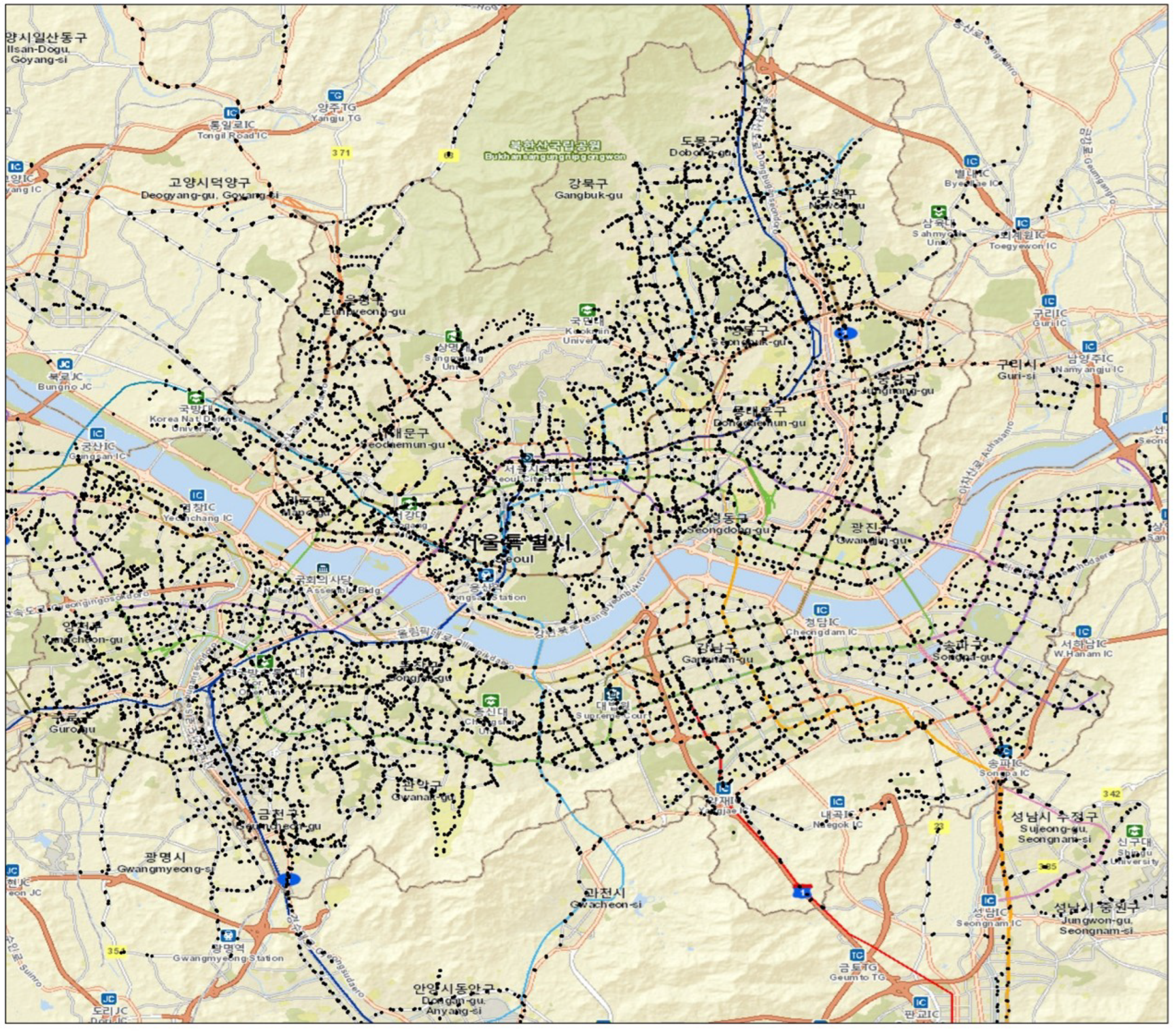
All the metro and bus routes within the Seoul metropolitan area are included in the AFC data. The stations and routes within the study area are shown in Figure 1. AFC data consist of 12 weeks of rider transactions: one week of each month of the year 2013. During those 12 weeks, the city of Seoul operated 18 metro lines and 11,637 buses over 936 routes, and 1,101,544,931 transactions and 35,978,530 unique smart card IDs were recorded. Each AFC record has travel information such as card ID, boarding and alighting stations and timestamps, route information, etc. More details (specific inputs and relevant data processing) about the dataset can be found in the authors’ earlier work [49,50].
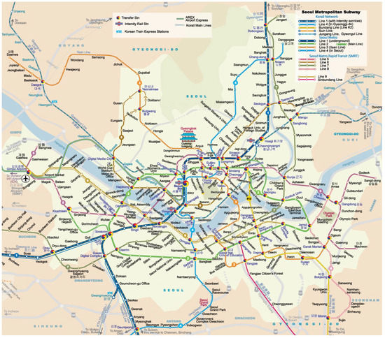

Figure 1.
Metro map (source: Johomaps) and bus map in Seoul.
In this study, unless specified, we only used weekday data from the third week of March 2013 to illustrate the human-mobility patterns of public-transportation smart card users.
4. Empirical Observations
4.1. User Groups and Travel Statistics
Transit card users are classified into 10 groups; however, only four groups constitute the majority of transit users. From largest to smallest, the four groups are regular users, middle- and high-school students, seniors, and card holders with disabilities. Here, the regular group refers to the card users that do not belong to any other nine groups. Since around 99% of the total transit card users are from these four groups, we focused on analyzing their mobility patterns. Table 1 presents the number of unique card IDs, the number of trip transactions made, and the daily travel time of user groups. The number of card IDs is not necessarily equal to the number of card users, because there may be one-time cards used during a week—however, we treated each unique ID as one traveler. We can also find out that the number of transactions are basically proportionate to the number of card IDs. AFC data also showed that seniors’ and people with disabilities’ daily travel times are usually longer than the other two groups.

Table 1.
User group description and descriptive statistics.
Table 2 shows the travel characteristics of the top four groups of users. Within one week, most users across all population groups tend to travel more frequently on weekdays compared to weekends. If they swipe their cards during weekends as often as weekdays, the weekday/weekend ratio should be close to 2.5. However, the ratios for all four groups were much higher than 2.5. Compared to the regular users, students travel more often on weekends.
Table 2.
Number of transactions by day of the week.
Modal preferences (Table 3) vary across population groups. Regular riders have similar shares for traveling on buses and metro trains. However, students prefer buses more since buses are ideal for short distance traveling, and students usually live near the schools. On the other hand, seniors and passengers with disabilities usually prefer metros when traveling within the city since the metro is free for seniors and people with disabilities.
Table 3.
Number of transactions by transportation mode.
For weekdays, we defined 6:00 a.m. to 10:00 a.m. as morning peak hours (MP), 4:00 p.m. to 8:00 p.m. as afternoon peak hours (AP), and all remaining time as non-peak hours (NP). We also defined a trip of a user as the combination of transactions between his or her origin and the final destination. The reason is that sometimes a passenger transfers between modes in order to reach his or her final destination, but the transactions of this trip will be recorded separately. A transfer needs to occur within 30 min, and there is little to no charge for transfers.
As shown in Table 4, only around 30% of trips of regular and student groups are made during non-peak hours. However, the percentage is higher for seniors and people with disabilities. The transfer time is the time spent to transfer between routes, modes, or stations. It is usually higher during non-peak hours since the headway of the bus and metro is shorter. Students have overall the shortest travel time among all groups. They spend less time on buses and the metro when traveling. Compared to seniors and the people with disabilities groups, regular users have a slightly lower travel time over all times of day.
Table 4.
Travel time, transfer time, travel cost, and number of transfers per trip by time of day by transportation mode.
In Seoul, students pay a discounted fare on both modes of transportation. For seniors and people with disabilities, taking the metro is free but taking the bus is not. This is one of the reasons why the metro is highly popular among these two population groups. We also found that the travel distance for all groups were similar during peak and non-peak hours, since the travel time and travel cost did not change much with the time changes.
The data shows that seniors and individuals with disabilities usually choose routes with fewer transfers (see Table 4). Regular users and students, on average, transfer twice as often as the other two groups. In terms of the time per transfer, we can see that the senior group has longer transfers every time, sometimes even twice as long as the regular and student groups.
We also measured destination variety and regularity (the last two columns of Table 4) to understand mobility patterns. Destination variety is defined as the number of unique destinations a traveler visited during a time period. We found that the variety was decreasing in the order of the regular, student, and people-with-disabilities groups. Destination variety is higher during weekdays than weekends. For weekends, this variety is much lower on Saturdays. On an hourly scale, we found the variety is much higher during 5:00–9:00 a.m. on weekdays. The groups with the highest variety during peak hours are usually the regular and student groups. However, the senior group has a high destination variety during non-peak hours.
Destination regularity measures how regularly a passenger visits his/her frequent destinations during each hour. Here, “frequent destination” is defined as the most-frequently-visited destination for this traveler during the same hour for all weekdays.
The set of all the destinations traveler t visited during hour h is denoted as , for all weekdays. The most-visited destination during hour h for traveler t is denoted as . is denoted as a function to calculate the number of records in the AFC database, which indicates that traveler t travels to destination during hour h. Then, destination regularity () for traveler t during hour h will be calculated as:
For each traveler t, we used the average value to represent his/her daily, morning-peak-hour (MP), afternoon-peak-hour (AP), and non-peak-hour (NP) destination regularity. Thus, hour set for these four time periods is: or or or . A higher destination regularity value indicates a more regular and predictable pattern of their daily/MP/AP/NP travel activity. For the regular and student user groups, the destination regularity value is low during the middle of the day. However, destination regularity for the other two groups is relatively higher, especially during peak hours.
4.2. Home and Workplace Identification
For each individual user, visited stations can be ranked based on the frequency of visits. In addition, studies [3] have shown that the most-visited stations are usually near their daily commuting locations, such as homes and work places. We developed some heuristic rules to identify a transit user’s potential home, work, and other activity locations. The rules are as follows:
- Homes are defined as the most-departed station during morning peak hours as well as the most-visited station during afternoon peak hours.
- Work places are defined as the most-visited station during morning peak hours as well as the most-departed station during afternoon peak hours. Work places may be schools for user group 4, students. These may be daily routine places for some users, including shopping, social, or recreational functions. However, they are all referred to as “workplaces” in this study.
- Other activity locations are defined as the most-visited stations during non-peak hours. They may be the places for shopping, recreational, or social purposes.
4.3. Spatial Patterns of Human Mobility
Figure 2 presents the spatial distributions of potential home, work, and other activity locations. Most of the potential home locations are concentrated in the northeast and southwest urban fringe areas (a,d). These two clusters are more preferred by seniors and users with disabilities as their home locations (g,j). However, the work locations for regular users are agglomerated near central city areas of Seoul (b). School locations are basically scattered all over the city (e). Daily routine places for seniors and people with disabilities are clustered near home as well as the central city areas (h,k). The distribution of other activity locations is similar among the four groups, although the purpose of these trips are various. These places are normally located between home and work locations (c,f,i,l).
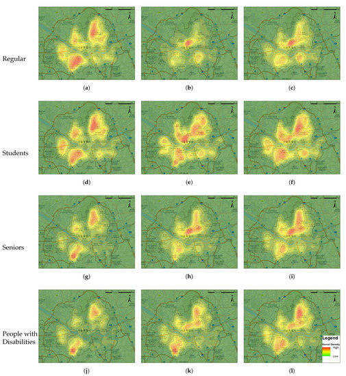
Figure 2.
Distributions of potential home, workplaces, and other activity locations in Seoul.
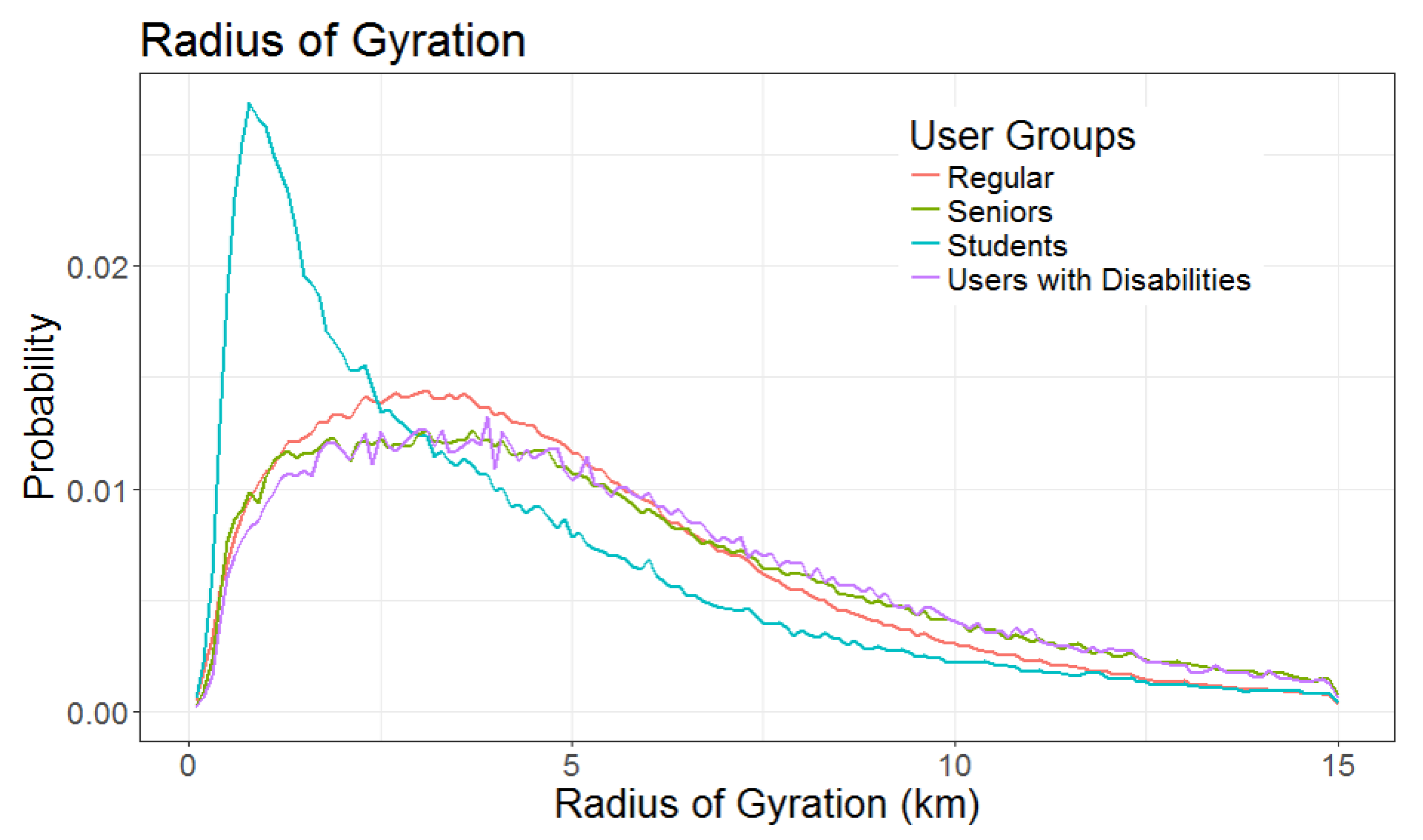
The radius of gyration measures the standard deviation of distances between users’ traveled stations and stations’ centers of mass. It measures the frequency and distance of a user’s mobility. A high radius of gyration value indicates that the user moves longer distances, while a low value of radius of gyration shows a short range of movements. It is defined as
in which n is the number of stations a user travels, and is the distance between station and center of mass . Figure 3 shows that, on average, the radius of gyration for students is significantly shorter than that of the other three groups. For seniors and riders with disabilities, the radius of gyration is not as affected by their identity, compared to the regular group of users.
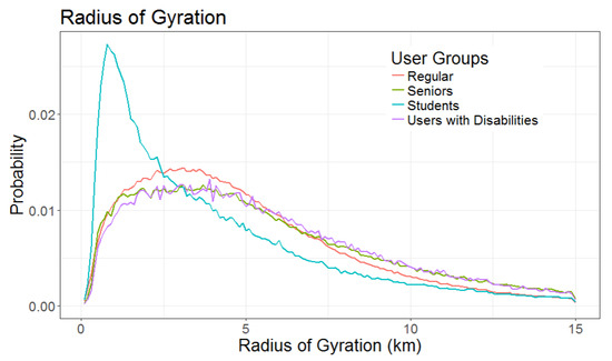
Figure 3.
Radius of gyration by user groups.
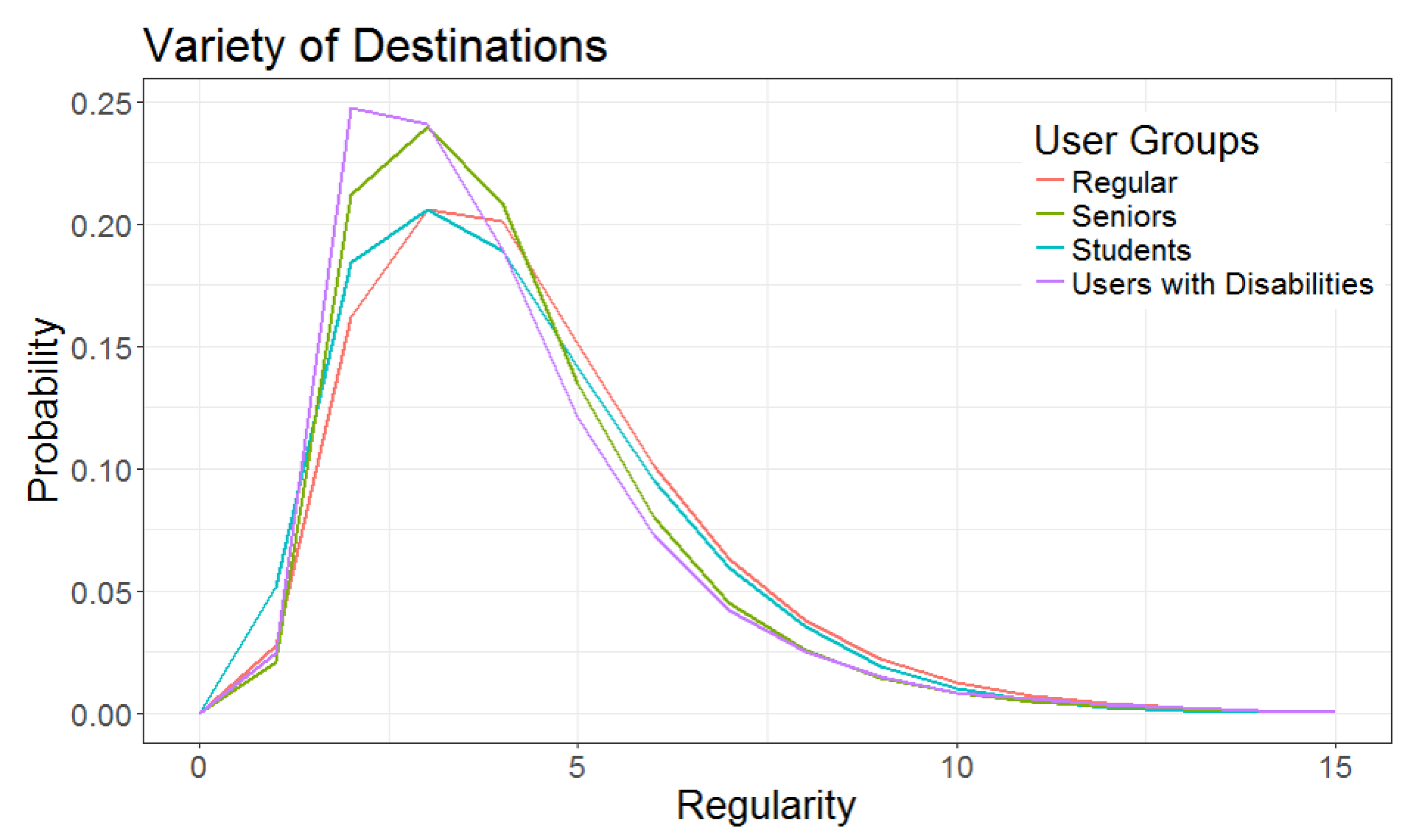
The number of unique destinations is also a spatial measurement of human mobility (Figure 4). Overall, the frequency distribution of the “number of distinct destinations visited” by each age group shows a power-law pattern. Most of the public transit users only visit two to four destinations per week. The average destination variety is various among different age groups. It is decreasing in the order of regular, student, senior, and people-with-disabilities-population groups, but the difference is not obvious.
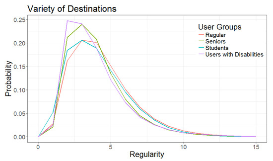
Figure 4.
Variety of destination by user groups.
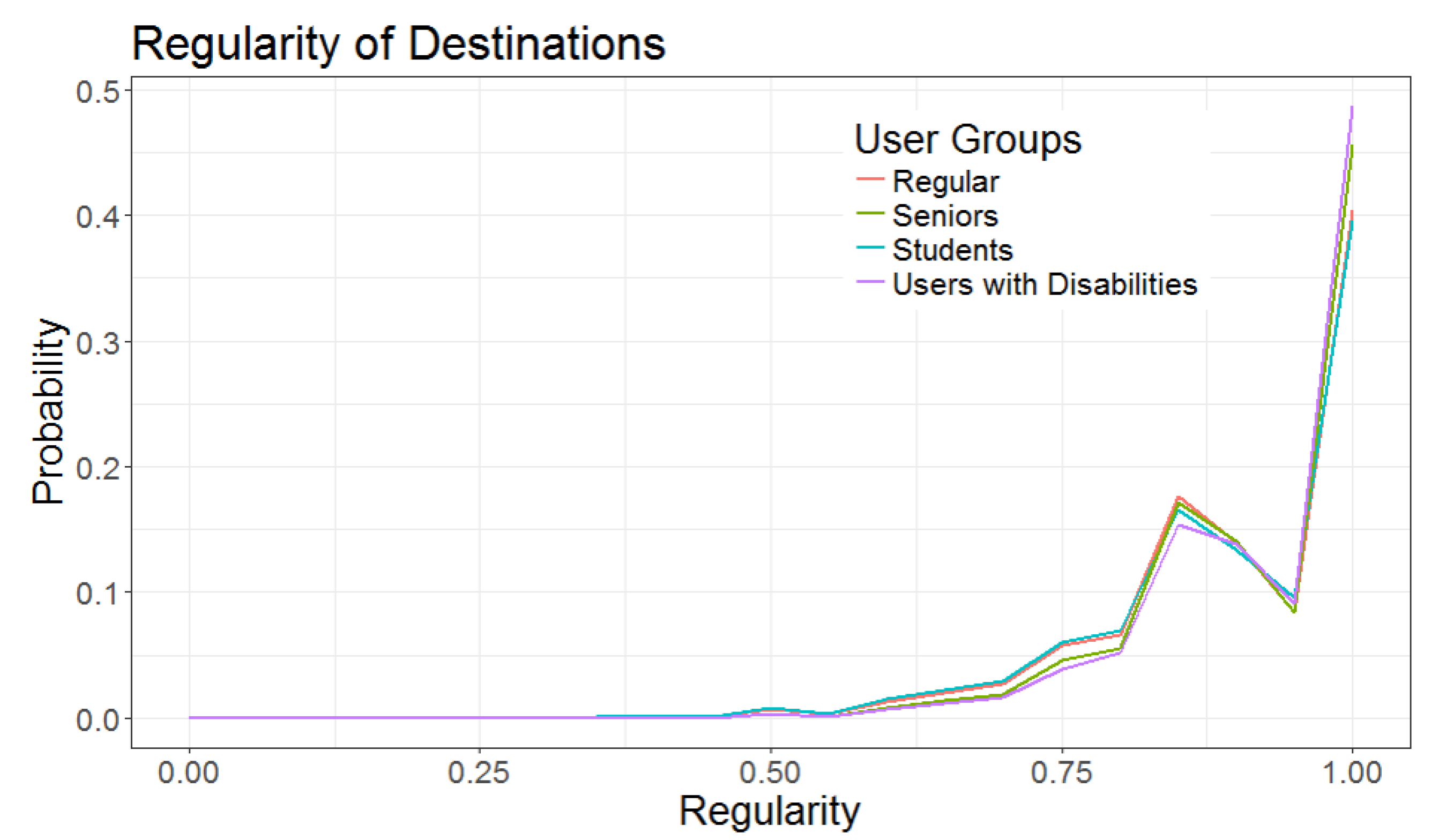
Destination-regularity measures the hourly percentages of the most-visited destinations (Figure 5). The frequency graph shows that most of the travelers have a high repeated pattern of destinations, and most of the regularity is between 0.8 and 1. Their most-visited places are more than 80% of all the destinations they have visited according to their travel history. People with disabilities, seniors, and students have higher destination regularity compared with the regular smart-card users.
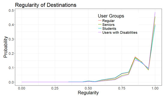
Figure 5.
Regularity of destination by user groups.
4.4. Temporal Patterns of Human Mobility
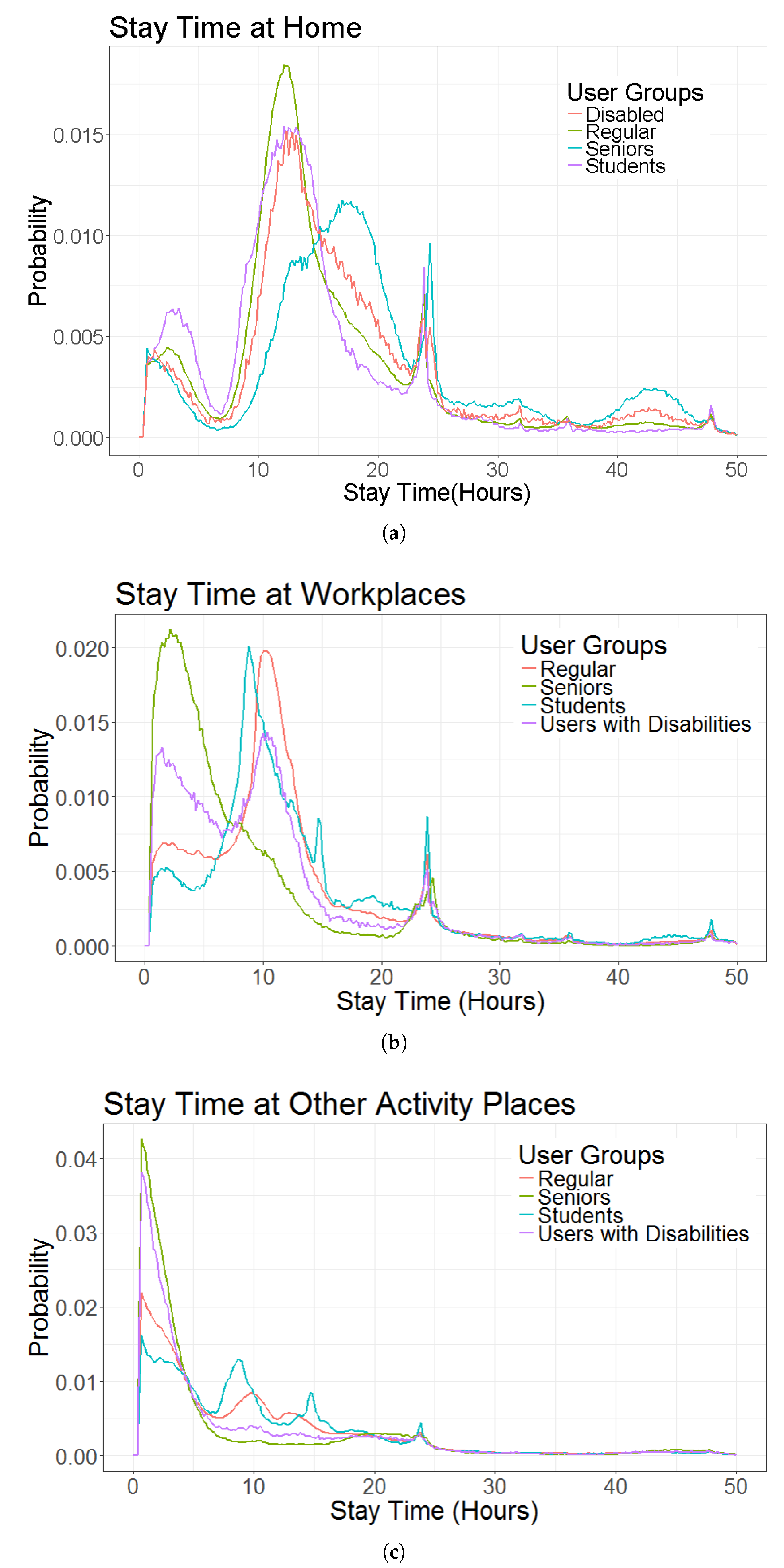
Figure 6 shows the temporal mobility patterns of transit riders. As shown in Figure 6a, the distributions of stay time at home for different user groups are usually different. For regular users, students, and people with disabilities, there is a peak around 12 h, indicating a typical stay time at home for these users. Seniors have a longer typical stay time at home. All user groups have peaks at a very short time in their stay time distributions. These 1 to 2 h could represent lunch breaks or the breaks between arriving home in the afternoon and leaving for recreational, social, shopping, or extracurricular activities (for student groups) purposes in the evening.

Figure 6.
Stay time at home, workplaces, and recreational places by user groups.
The differences of stay times at work locations are even greater across groups (see Figure 6b). Regular users and students usually stay at work places or schools for 9–10 h. However, most of the seniors will stay at their daily routine places for 2–3 h per day. People with disabilities are unique because the distribution has two peaks in terms of the stay time. Nearly half of them stay at work locations for 10 h, but the other half only leave home for less than one hour per day. If a card user with disabilities has a job, this individual probably will stay at his/her workplace around 10 h, just like a regular user. However, if a card user with disabilities does not have a job, he/she will tend to make short trips during the day. Figure 6c shows that all groups usually spend less than four hours for other activities per day.
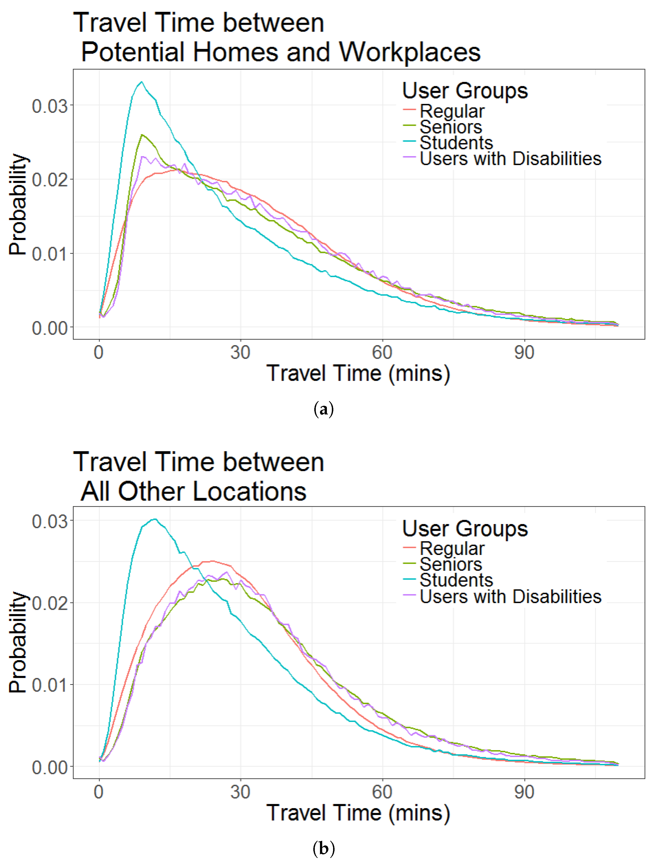
In Figure 7a, we observe that regular users, seniors, and people with disabilities usually take about 10 more minutes than students to travel between their homes and workplaces. This information implies that schools are usually close to home compared to work places.
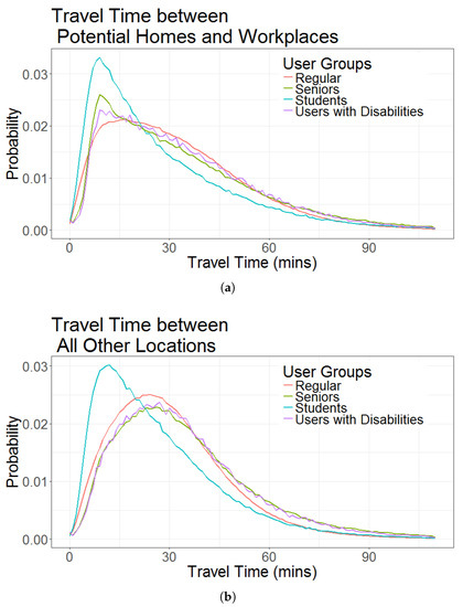
Figure 7.
Time between two most-visited places and all other locations by user groups.
Students also spend less time traveling between places other than home and schools, as shown in Figure 7b. The reason is that students often do not go too far away from home and schools. Unlike other adult groups, the daily activity region of students is much smaller. It can also be confirmed from the results of comparing the radius of gyration across groups.
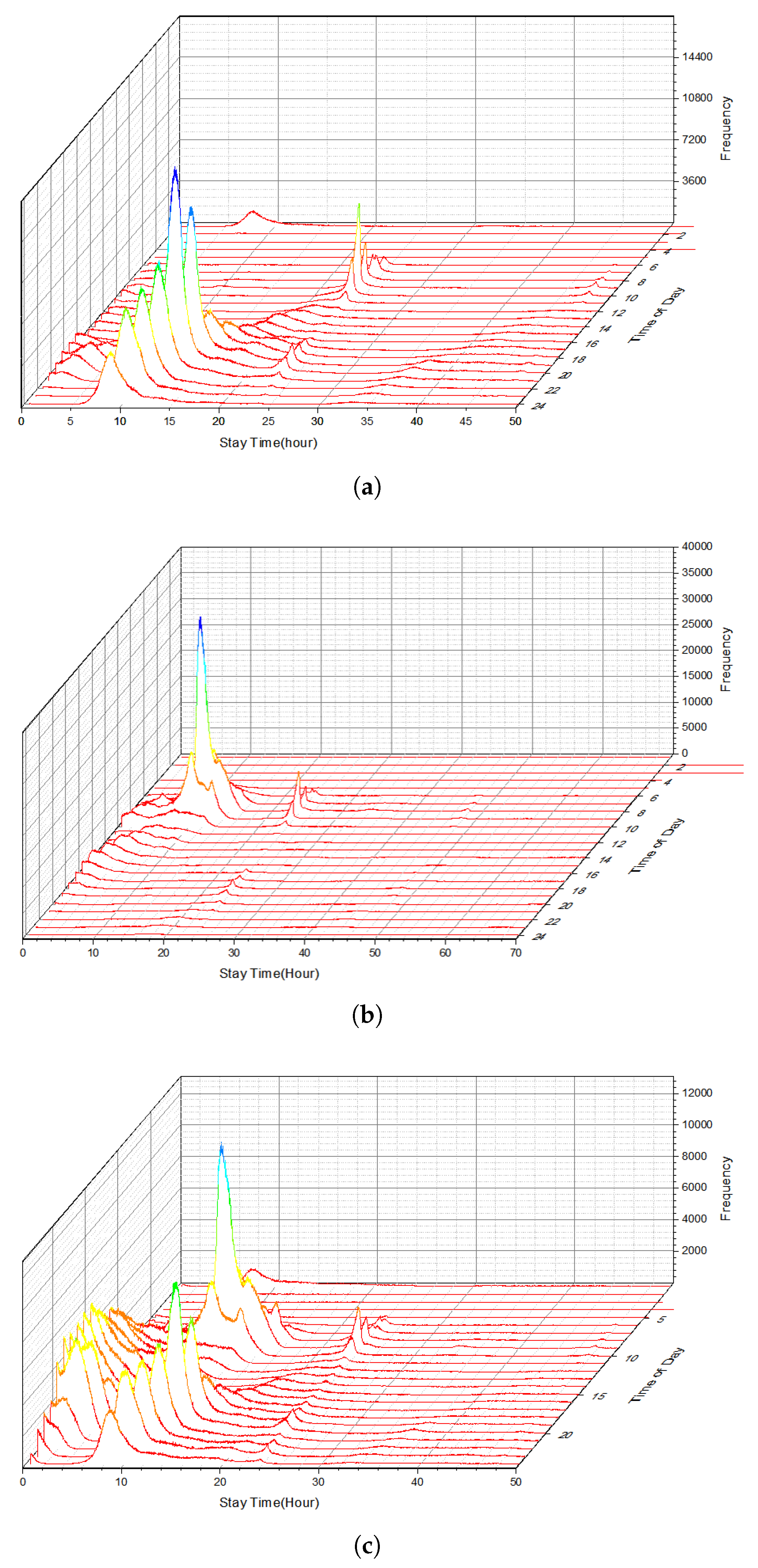
Figure 8 shows that the distribution of stay time varies based on the time of day. Usually, from morning to afternoon, the earlier a user reaches home, the longer the stay time is. This pattern is reversed from afternoon to midnight. From morning to afternoon, the later a user arrives at a workplace, the shorter the stay time is. Users will stay less than 4 h in other activity locations during non-peak hours. This changing pattern by time of day is applicable for all user groups.
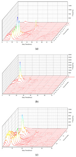
Figure 8.
3D waterfall graph of stay time at home, workplaces, and other activity locations.
4.5. Heterogeneity among Mobility Patterns
Although we could observe the differences of travel behaviors through the above distribution figures, it is still necessary to measure and compare them statistically. In order to measure the heterogeneity of stay time, travel time and radius of gyration distributions across various smart card user groups, the best fit of distributions needs to be decided and the parameters need to be estimated and compared. Previous studies indicate that most of the displacements and pauses follow power-law, exponential, or log-normal distributions [32]. By comparing, we found that the log-normal distribution had the highest log-likelihood and the lowest Akaike Information Criterion (AIC) value. HA hgher log-likelihood is usually preferred when using the maximum-likelihood technique to fit the data with statistical models. AIC is a measurement of the relative quality of a model. The one with the minimum AIC value is normally the best model among candidate models. It has been shown that a log-normal distribution is a statistically better fit for describing the distributions of stay time, travel time, and radius of gyration for all population groups.
As shown in Table 5, for the stay time at home, all four groups had similar estimated parameters. The only exception is group 6 (seniors), which had the largest mean and standard deviation. It means that the senior group tend to stay longer at home, which could be confirmed by observing Figure 6a. For the stay time at workplaces, regular and student groups shared similar estimated parameters. Seniors and people with disabilities usually stay less time at their “workplaces,” and this is also true if we check Figure 6b. For the stay time and other activity locations, there are still two type of patterns: regular/student groups and senior/people with disability groups (also see Figure 6c). Regular/student groups have a longer stay time but a lower standard deviation, while senior/people-with-disabilities groups have a shorter stay time but higher standard deviation. Nevertheless, the heterogeneity exists across groups in terms of the stay time at various important daily locations.
Table 5.
Estimated parameters of distributions.
Except for the student group, all three other groups shared a similar distribution for travel time between commuting locations. Students usually traveled closer to home compared to the other groups. The mean of the distribution was smaller, but the standard deviation was higher. This behavior can also be observed from Figure 7. The distribution of the radius of gyration for the student group also stands out in the four groups. It had a smaller mean and a higher standard deviation.
We present the results of the Kolmogorov–Smirnov test for pair-wise comparison of distribution. The Kolmogorov–Smirnov test is a non-parametric test of the equality of two distributions. All of the results showed p-values that are less than 0.001. This data mean that, statistically, none of all the pair-wise comparison of two distributions can be stated as equality (Table 6).
Table 6.
p value from Kolmogorov–Smirnov test, all significant at = 0.001 level.
5. Conclusions
This study presented the heterogeneity of spatial and temporal mobility patterns across user-demographic groups. We analyzed large-scale data (4.7 million users) of AFC records of the public-transportation system of Seoul, South Korea. The empirical findings of this study provide us with useful insights on human-mobility behaviors across different population groups. First, departure-time, travel-mode, and activity-duration choices differed across socio-demographic groups. Second, the spatial distribution of each group’s potential home, work ,and other activity locations were different. Lastly, the heterogeneity of displacement and pause distributions were statistically significant.
The observations we found for each demographic group are summarized as follows:
- Overall, public-transit users travel more often on weekdays than weekends; their homes and workplaces are clustered.
- The regular group mostly consists of adults with jobs. They have typical home-to-work trips during weekdays and recreational activities during non-work hours (evenings and weekends). This is the base group to which other groups will be compared.
- The student-group users often choose to take buses rather than the metro and travel more often in peak hours. They have a lower daily travel cost due to their short daily travel time/distance and fare discount. Furthermore, their trips show patterns of a high destination regularity, a low radius of gyration, and a short travel time of work (school) trips.
- The senior-group travelers often choose to take the metro because it is free for them and the bus is not. Other reasons may include the accessibility of bus stops, wheel-chair accessibility of buses, etc. They travel more often in non-peak hours, potentially to avoid congestion and crowds. Their trips have fewer transfers, a longer transfer time per transfer, a slightly higher daily travel time, a low destination variety and, overall, a higher destination regularity, a longer stay time at home, and a shorter stay time at other places.
- People with disabilities often choose to take the metro because it is free for them and the bus is not. They travel more often in non-peak hours. Their trips have fewer transfers, a longer transfer time per transfer, a slightly higher daily travel time, a low destination variety overall, and a high destination regularity. Their stay time at daily routine places are bi-modal distributed. Our assumption was that this bi-modal distribution is probably caused by whether they have jobs. If they need to work during daylight hours, their stay time at daily-routine places is around 10 h, and this daily-routine place is actually their workplace. If they are not employed, the stay time at daily-routine places is much shorter, and their mobility pattern looks more like that of the senior group than that of the regular group.
Despite strong differences in human-mobility patterns across different groups, heterogeneity in mobility behavior has been ignored in previous studies describing and modeling universal human-mobility behavior using trajectory datasets due to the difficulties of identifying user groups of individuals [3,32]. Mobility patterns are different for minor user groups such as students, seniors, and the people-with-disabilities population. Understanding it will help us better characterize individual mobility dynamics and develop high-resolution models to predict realistic individual movements in space and time. Further, such information can lead to better decision making in certain applications such as transportation planning, urban design, policy making, etc. Such further research can explore specific applications that can make better decisions from understanding heterogeneity in human-mobility behaviors. For example, based on the findings, we can further analyze how public-transit-pricing strategies can cater to different groups of users and their preferences, or, one can explore how urban design and land use have impacted destination choices among different user groups.
Author Contributions
Conceptualization, J.E.K. and S.H.; methodology, S.H.; formal analysis, L.W.; investigation, L.W.; resources, Y.C.; data curation, L.W.; writing—original draft preparation, L.W.; writing—review and editing, J.E.K. and S.H.; visualization, L.W.; supervision, J.E.K. and S.H.; funding acquisition, J.E.K. All authors have read and agreed to the published version of the manuscript.
Funding
This research was funded by the US National Science Foundation grant number CMMI-1636602.
Institutional Review Board Statement
Not applicable.
Informed Consent Statement
Not applicable.
Data Availability Statement
AFC data used for this research cannot be shared. The AFC dataset was provided for the research team for specific research purposes.
Conflicts of Interest
The authors declare no conflict of interest.
Abbreviations
The following abbreviations are used in this manuscript:
| AFC | Automatic Fare Collection |
| OD | Origin–Destination |
| GPS | Global Positioning System |
References
- Hasan, S.; Ukkusuri, S.V. Reconstructing Activity Location Sequences From Incomplete Check-In Data: A Semi-Markov Continuous-Time Bayesian Network Model. IEEE Trans. Intell. Transp. Syst. 2017, 19, 687–698. [Google Scholar] [CrossRef]
- Barbosa, H.; Barthelemy, M.; Ghoshal, G.; James, C.R.; Lenormand, M.; Louail, T.; Menezes, R.; Ramasco, J.J.; Simini, F.; Tomasini, M. Human mobility: Models and applications. Phys. Rep. 2018, 734, 1–74. [Google Scholar] [CrossRef] [Green Version]
- Hasan, S.; Schneider, C.M.; Ukkusuri, S.V.; González, M.C. Spatiotemporal Patterns of Urban Human Mobility. J. Stat. Phys. 2013, 151, 304–318. [Google Scholar] [CrossRef] [Green Version]
- Sun, L.; Lee, D.H.; Erath, A.; Huang, X. Using smart card data to extract passenger’s spatio-temporal density and train’s trajectory of MRT system. In Proceedings of the ACM SIGKDD International Workshop on Urban Computing, Beijing, China, 12 August 2012; pp. 142–148. [Google Scholar]
- Brockmann, D.; Hufnagel, L.; Geisel, T. The scaling laws of human travel. Nature 2006, 439, 462–465. [Google Scholar] [CrossRef]
- González, M.C.; Hidalgo, C.A.; Barabási, A.L. Understanding individual human mobility patterns. Nature 2008, 453, 779–782. [Google Scholar] [CrossRef] [PubMed]
- Liu, Y.; Sui, Z.; Kang, C.; Gao, Y. Uncovering patterns of inter-urban trip and spatial interaction from social media check-in data. PLoS ONE 2014, 9, e86026. [Google Scholar] [CrossRef] [PubMed]
- Zhao, K.; Musolesi, M.; Hui, P.; Rao, W.; Tarkoma, S. Explaining the power-law distribution of human mobility through transportation modality decomposition. Sci. Rep. 2015, 5, 9136. [Google Scholar] [CrossRef] [PubMed] [Green Version]
- Stouffer, S.A. Intervening opportunities: A theory relating mobility and distance. Am. Sociol. Rev. 1940, 5, 845–867. [Google Scholar] [CrossRef]
- Noulas, A.; Scellato, S.; Lambiotte, R.; Pontil, M.; Mascolo, C. A tale of many cities: Universal patterns in human urban mobility. PLoS ONE 2012, 7, e37027. [Google Scholar] [CrossRef]
- Riccardo, G.; Armando, B.; Sandro, R. Towards a statistical physics of human mobility. Int. J. Mod. Phys. C 2012, 23, 1250061. [Google Scholar] [CrossRef] [Green Version]
- Wang, W.; Pan, L.; Yuan, N.; Zhang, S.; Liu, D. A comparative analysis of intra-city human mobility by taxi. Phys. A Stat. Mech. Its Appl. 2015, 420, 134–147. [Google Scholar] [CrossRef]
- Tang, J.; Liu, F.; Wang, Y.; Wang, H. Uncovering urban human mobility from large scale taxi GPS data. Phys. A Stat. Mech. Its Appl. 2015, 438, 140–153. [Google Scholar] [CrossRef]
- Pas, E.I. The effect of selected sociodemographic characteristics on daily travel-activity behavior. Environ. Plan. A 1984, 16, 571–581. [Google Scholar] [CrossRef]
- Vredin, J.M.; Heldt, T.; Johansson, P. The effects of attitudes and personality traits on mode choice. Transp. Res. Part A Policy Pract. 2006, 40, 507–525. [Google Scholar] [CrossRef] [Green Version]
- Hanson, S.; Hanson, P. The travel-activity patterns of urban residents: Dimensions and relationships to sociodemographic characteristics. Econ. Geogr. 1981, 57, 332–347. [Google Scholar] [CrossRef]
- Salomon, I. Life styles—A broader perspective on travel behavior. In Recent Advances in Travel Demand Analysis; Gower: Aldershot, UK, 1983; pp. 290–310. [Google Scholar]
- Kitamura, R. Life-style and travel demand. Transportation 2009, 36, 679–710. [Google Scholar] [CrossRef] [Green Version]
- Hasan, S.; Ukkusuri, S.V. Location Contexts of User Check-ins to Model Urban Geo Life-Style Patterns. PLoS ONE 2015, 10, e0124819. [Google Scholar] [CrossRef]
- Ritter, A.S.; Straight, A.; Evans, E.L. Understanding Senior Transportation: Report and Analysis of a Survey of Consumers Age 50; AARP, Public Policy Institute: Washington, DC, USA, 2002. [Google Scholar]
- Coughlin, J. Transportation and Older Persons: Perceptions and Preferences: A Report on Focus Groups. 2001. Available online: https://trid.trb.org/view/723956 (accessed on 11 November 2021).
- Risser, R.; Haindl, G.; Ståhl, A. Barriers to senior citizens’ outdoor mobility in Europe. Eur. J. Ageing 2010, 7, 69–80. [Google Scholar] [CrossRef] [PubMed]
- Wretstrand, A.; Svensson, H.; Fristedt, S.; Falkmer, T. Older people and local public transit: Mobility effects of accessibility improvements in Sweden. J. Transp. Land Use 2009, 2, 49–65. [Google Scholar] [CrossRef]
- Collia, D.V.; Sharp, J.; Giesbrecht, L. The 2001 national household travel survey: A look into the travel patterns of older Americans. J. Saf. Res. 2003, 34, 461–470. [Google Scholar] [CrossRef] [PubMed]
- Newbold, K.B.; Scott, D.M.; Spinney, J.E.; Kanaroglou, P.; Páez, A. Travel behavior within Canada’s older population: A cohort analysis. J. Transp. Geogr. 2005, 13, 340–351. [Google Scholar] [CrossRef]
- Schmöcker, J.D.; Quddus, M.A.; Noland, R.B.; Bell, M.G. Estimating trip generation of elderly and disabled people: Analysis of London data. Transp. Res. Rec. 2005, 1924, 9–18. [Google Scholar] [CrossRef]
- Mercado, R.; Páez, A. Determinants of distance traveled with a focus on the elderly: A multilevel analysis in the Hamilton CMA, Canada. J. Transp. Geogr. 2009, 17, 65–76. [Google Scholar] [CrossRef]
- Van den Berg, P.; Arentze, T.; Timmermans, H. Estimating social travel demand of senior citizens in the Netherlands. J. Transp. Geogr. 2011, 19, 323–331. [Google Scholar] [CrossRef]
- Mattson, J.W. Travel Behavior and Mobility of Transportation-Disadvantaged Populations: Evidence from the National Household Travel Survey; Technical Report; Upper Great Plains Transportation Institute: Fargo, ND, USA, 2012. [Google Scholar]
- Calabrese, F.; Diao, M.; Di Lorenzo, G.; Ferreira, J.; Ratti, C. Understanding individual mobility patterns from urban sensing data: A mobile phone trace example. Transp. Res. Part C Emerg. Technol. 2013, 26, 301–313. [Google Scholar] [CrossRef]
- Iqbal, M.S.; Choudhury, C.F.; Wang, P.; González, M.C. Development of origin-destination matrices using mobile phone call data. Transp. Res. Part C Emerg. Technol. 2014, 40, 63–74. [Google Scholar] [CrossRef] [Green Version]
- Alessandretti, L.; Sapiezynski, P.; Lehmann, S.; Baronchelli, A. Multi-scale spatio-temporal analysis of human mobility. PLoS ONE 2017, 12, e0171686. [Google Scholar] [CrossRef] [Green Version]
- Jiang, S.; Ferreira, J.; Gonzalez, M.C. Activity-based human mobility patterns inferred from mobile phone data: A case study of Singapore. IEEE Trans. Big Data 2017, 3, 208–219. [Google Scholar] [CrossRef] [Green Version]
- Cheng, Z.; Caverlee, J.; Lee, K.; Sui, D.Z. Exploring millions of footprints in location sharing services. In Proceedings of the 5th International AAAI Conference on Weblogs and Social Media (ICWSM), Barcelona, Spain, 17–21 July 2011. [Google Scholar]
- Hasan, S.; Zhan, X.; Ukkusuri, S.V. Understanding urban human activity and mobility patterns using large-scale location-based data from online social media. In Proceedings of the 2nd ACM SIGKDD International Workshop on Urban Computing, Chicago, IL, USA, 11 August 2013. [Google Scholar]
- Yang, F.; Jin, P.J.; Wan, X.; Li, R.; Ran, B. Dynamic Origin-Destination Travel Demand Estimation using Location Based Social Networking Data. In Proceedings of the 93rd Annual Meeting of Transportation Research Board, Washington, DC, USA, 12–16 January 2014. Number 14-5509. [Google Scholar]
- Spyratos, S.; Vespe, M.; Natale, F.; Weber, I.; Zagheni, E.; Rango, M. Quantifying international human mobility patterns using Facebook Network data. PLoS ONE 2019, 14, e0224134. [Google Scholar] [CrossRef] [PubMed] [Green Version]
- Han, S.Y.; Tsou, M.H.; Knaap, E.; Rey, S.; Cao, G. How do cities flow in an emergency? Tracing human mobility patterns during a natural disaster with big data and geospatial data science. Urban Sci. 2019, 3, 51. [Google Scholar] [CrossRef] [Green Version]
- Medina, S.A.O. Inferring weekly primary activity patterns using public transport smart card data and a household travel survey. Travel Behav. Soc. 2016, 12, 93–101. [Google Scholar] [CrossRef] [Green Version]
- Xia, F.; Wang, J.; Kong, X.; Wang, Z.; Li, J.; Liu, C. Exploring human mobility patterns in urban scenarios: A trajectory data perspective. IEEE Commun. Mag. 2018, 56, 142–149. [Google Scholar] [CrossRef]
- Jin, P.J.; Cebelak, M.; Yang, F.; Ran, B.; Walton, C.M.; Zhang, J. Location-Based Social Networking Data: Exploration of Use of Doubly Constrained Gravity Model for Origin-Destination Estimation. In Proceedings of the 93rd Annual Meeting of Transportation Research Board, Washington, DC, USA, 12–16 January 2014. Number 14-5314. [Google Scholar]
- Zhou, X.; Mahmassani, H.S. A structural state space model for real-time traffic origin–destination demand estimation and prediction in a day-to-day learning framework. Transp. Res. Part B Methodol. 2007, 41, 823–840. [Google Scholar] [CrossRef]
- Barry, J.; Newhouser, R.; Rahbee, A.; Sayeda, S. Origin and destination estimation in New York City with automated fare system data. Transp. Res. Rec. J. Transp. Res. Board 2002, 1817, 183–187. [Google Scholar] [CrossRef]
- Zhao, J. The Planning and Analysis Implications of Automated Data Collection Systems: Rail Transit OD Matrix Inference and Path Choice Modeling Examples. Ph.D. Thesis, Massachusetts Institute of Technology, Cambridge, MA, USA, 2004. [Google Scholar]
- Cui, A. Bus Passenger Origin-Destination Matrix Estimation Using Automated Data Collection Systems. Master’s Thesis, Massachusetts Institute of Technology, Cambridge, MA, USA, 2006. [Google Scholar]
- Sun, L.; Lu, Y.; Jin, J.G.; Lee, D.H.; Axhausen, K.W. An integrated Bayesian approach for passenger flow assignment in metro networks. Transp. Res. Part C Emerg. Technol. 2015, 52, 116–131. [Google Scholar] [CrossRef]
- Park, J.; Kim, D.J.; Lim, Y. Use of smart card data to define public transit use in Seoul, South Korea. Transp. Res. Rec. J. Transp. Res. Board 2008, 2063, 3–9. [Google Scholar] [CrossRef]
- Jang, W. Travel time and transfer analysis using transit smart card data. Transp. Res. Rec. J. Transp. Res. Board 2010, 2144, 142–149. [Google Scholar] [CrossRef]
- Wu, L.; Kang, J.E.; Chung, Y.; Nikolaev, A. Monitoring multimodal travel environment using automated fare collection data: Data processing and reliability analysis. J. Big Data Anal. Transp. 2019, 1, 123–146. [Google Scholar] [CrossRef] [Green Version]
- Wu, L.; Kang, J.E.; Chung, Y.; Nikolaev, A. Inferring origin-Destination demand and user preferences in a multi-modal travel environment using automated fare collection data. Omega 2021, 101, 102260. [Google Scholar] [CrossRef]


Publisher’s Note: MDPI stays neutral with regard to jurisdictional claims in published maps and institutional affiliations. |
© 2021 by the authors. Licensee MDPI, Basel, Switzerland. This article is an open access article distributed under the terms and conditions of the Creative Commons Attribution (CC BY) license (https://creativecommons.org/licenses/by/4.0/).