Solving the Real Power Limitations in the Dynamic Economic Dispatch of Large-Scale Thermal Power Units under the Effects of Valve-Point Loading and Ramp-Rate Limitations

Abstract

Few non-traditional optimization techniques are applied to the dynamic economic dispatch (DED) of large-scale thermal power units (TPUs), e.g., 1000 TPUs, that consider the effects of valve-point loading with ramp-rate limitations. This is a complicated multiple mode problem. In this investigation, a novel optimization technique, namely, a multi-gradient particle swarm optimization (MG-PSO) algorithm with two stages for exploring and exploiting the search space area, is employed as an optimization tool. The M particles (explorers) in the first stage are used to explore new neighborhoods, whereas the M particles (exploiters) in the second stage are used to exploit the best neighborhood. The M particles’ negative gradient variation in both stages causes the equilibrium between the global and local search space capabilities. This algorithm’s authentication is demonstrated on five medium-scale to very large-scale power systems. The MG-PSO algorithm effectively reduces the difficulty of handling the large-scale DED problem, and simulation results confirm this algorithm’s suitability for such a complicated multi-objective problem at varying fitness performance measures and consistency. This algorithm is also applied to estimate the required generation in 24 h to meet load demand changes. This investigation provides useful technical references for economic dispatch operators to update their power system programs in order to achieve economic benefits.

1. Introduction

Although renewable power has been positively used in most power generating systems (PGSs), fossil fuels remain the predominant energy source for thermal power units (TPUs). The demand for fossil fuels continuously increases with the rapid growth of the global economy and modern industry. Thus, the increased efficiency and optimum utilization of fossil fuels in TPU operations have become important research topics. The scheduling of the correct mix of PGS generation from numerous online TPUs during a specific interval and load demand at minimum cost, i.e., economic dispatch (ED) of real power, is a challenging issue, because the real-time operating fuel costs (OFCs) of various online TPUs vary significantly.

The real power ED is the distribution of a total real power generation among the online TPUs, given that the commitment of online TPUs is pre-determined. Several studies have addressed the static ED problem; that is, the total real power generation is scheduled to cover the demand of loads for a specific hour [1,2,3,4,5,6,7,8]. However, the scheduling in such a case may be valuable only for that hour and may not be valid for the next hour or subsequent few hours, depending on the load demand changes during a 24 h period. For example, power generation delivered by online TPUs may not substantially change from one hour to the following operating hour due to the valve-point loading (VPL) effects and power limitations, namely, ramp-rate limitations (RRLs). This problem can be eliminated through the real-time dynamic scheduling of online TPUs to meet 24 h load demands in the presence of VPL effects and RRLs [9,10,11,12,13,14]. Real-time dynamic scheduling is recognized as the real-time dynamic economic dispatch (DED) of real power (DED problem) and minimizes the total OFC by satisfying the load demand in each period that may be 15, 30, or 60 min in 24 h and solving generation real power limitations, i.e., VPL effects and RRLs. A specific interval with 60 min has been selected in this investigation.

The OFC, that is, the multi-objective function of online TPU, is ideally a quadratic function, but a ripple is observed on this multi-objective function when the steam passes inside the valves of a steam turbine synchronous generator (STSG) [15,16,17,18,19]. Thus, the OFCs of a TPU become non-convex with multimodal characteristics [20,21,22,23]. The ramp real power limitations of a TPU are changed at each interval. Subsequently, the up/down RRLs pose an additional challenge to optimization techniques. Moreover, unexpected events, such as an online TPU fault or a sudden load demand change at any interval, occur. This problem is addressed by using the largest TPU capacity among online TPUs to maintain the overall online TPUs scheduling and increase system generation stability. However, an online TPU infers a solution from its optimum point. Therefore, finding the optimum scheduling for the DED of real power is a complicated PGS operation task. Because the DED of real power comprises 24 periods, each period is 1 h; thus, more decision variables than that in the static ED of real power are used for a dispatch period of 24 h. For example, a 500-TPU PGS has up to 12,000 (500 × 24) decision variables to be optimized. Thus, it is a big challenge to solve such a large-scale multi-objective DED problem.

Numerous optimization techniques for solving the DED problem have been applied, but few are positively used to solve the DED of large-scale TPUs with VPL effects and RRLs, that is, real power limitations. The optimization techniques in the literature are classified into traditional and non-traditional optimization techniques. Traditional optimization techniques, such as linear programming [24], the lambda iteration method [25], and the gradient method [26], have been widely utilized for solving the ED of real power. These optimization techniques are often efficient in solving the convex OFC function [27,28,29]. Traditional optimization techniques, including gradient methods, generally have disadvantages, such as inefficiency in solving convex problems with a high-dimensional search space, because they suffer from dimensionality. In addition, they are inefficient in solving non-convex multimodal problems and sensitive to an initial starting point. Moreover, they require a monotonically increasing objective function and often fall into the local minima [30,31,32]. However, the gradient method is invariably integrated with various optimization methods to develop novel optimization techniques. This integration is employed to obtain rapid convergence without falling in the local minimum. Some recently proposed optimization techniques are available in [33,34].

The second category includes non-traditional optimization techniques (NTOTs); they have been positively utilized in numerous practical optimization problems, because the mathematical specifications of an objective function are not essential. For example, evolutionary programming (EP) [4,9], the artificial immune system algorithm [35,36,37], the genetic algorithm (GA) [38,39,40], the artificial bee colony (ABC) [40,41,42], and particle swarm optimization (PSO) [42,43,44,45,46] have been proposed. A popular NTOT, namely, global PSO with the inertia weight (w) (GPSO-w) algorithm [47], has been proposed for solving unimodal and multimodal optimization problems, including the DED of real power. The negative gradient of w in the GPSO algorithm is employed to boost the particles’ local and global search abilities inside a swarm and enable equilibrium between the exploration and exploitation stages [48]. Thus, w helps the particles control the convergence characteristics and quickly converge into the optimum solution. Although the OFC function profile does not constrain it, the GPSO-w algorithm mostly falls in the local minima when applied to the ED of large-scale TPUs PGS with various operating power limitations [49,50,51].

Few NTOTs have been positively applied for solving the DED of large-scale TPUs with VPL effects and RRLs in the recent years, including the hybrid bare-bone PSO algorithm [1], the chaotic differential bee colony optimization (CDBCO) algorithm [14], the decentralized gradient projection method [15], the imperialist competitive algorithm (ICA) [16], the enhanced adaptive PSO (EAPSO) algorithm [17], the teaching–learning algorithm (TLA) [18], the orthogonal PSO algorithm [49], the crisscross optimization (CSO) algorithm [52], enhanced bee swarm optimization (EBSO) [53], the hybrid immune GA (HIGA) [54], the self-adaptive modified firefly algorithm [55,56], the chaotic sequence-based DE (CSDE) algorithm [57], the chaotic DE algorithm [58,59], the chaotic self-adaptive PSO algorithm [60], and the time-varying acceleration coefficient with improved PSO algorithm [61].

The results of these previous investigations emphasize the importance of studying the DED of the real power of large-scale TPUs. However, the current proposed research study’s advantage compared to the reviewed method in the literature satisfies the following steps:

(1)

Few NTOTs are used for the DED of large-scale TPUs, e.g., 1000 TPUs, that consider the effects of VPL with RRLs. The current study covers the lack in this field.

(2)

A novel algorithm, namely, a multi-gradient particle swarm optimization (MG-PSO) algorithm, is applied an optimization tool to solve the DED of 10 TPUs without/with transmission network loss; 100, 500 and, 1000 TPUs under VPL effects; and RRLs’ real power limitations.

(3)

The power generating scheduling of online TPUs is updated every 1 h for the duration of a day in a real-time operation to meet the load demands and real power limitations.

(4)

The generation is estimated to meet the load demand at any time during the period of a day. This procedure can maintain PGS stability and forecast the periodic maintenance schedule of the TPUs subjected to a massive change in their generation during the period of a day.

(5)

The research study provides details about the generation volume of each TPU over a 24 h period and which one is subjected to considerable changes during this period.

(6)

Most NTOTs in the literature often suffer from premature convergence and dimensionality when applied to a large-scale DED of real power (more than 500 TPUs) with many local minima due to the effects of VPL and RRLs. However, the MG-PSO algorithm was positively applied to alleviate particles’ convergence stagnancy even with 1000 TPUs throughout the solution’s inspections.

(7)

The approach used in the current research study is different from that adopted in our previous study [62,63]. In [62,63], the MG-PSO algorithm was used to solve the static ED for 1 h only of small and medium power systems, i.e., 6, 13, and 15 TPUs, under several power constraints, such as prohibited operating zones, RRLs, and VPL effects. However, in this study, the MG-PSO algorithm is used to solve the DED of large-scale TPUs, i.e., 100, 500, and 1000 TPUs, under the effects of VPL with RRLs during the 24 h period. It is a more complicated multi-objective function.

(8)

The GPSO-w algorithm is improved by using different negative gradient variations to prevent the best particle inside a swarm from falling in the local minimum and ensuring its escape.

(9)

With widespread simulated tests for the DED of medium-scale and large-scale TPU PGSs, the MG-PSO algorithm’s superiority over various competitive NTOTs, including the GPSO-w algorithm, in terms of performance measures has been demonstrated based on various numerous performance measures, such as fitness values, convergence rate, and consistency.

(10)

An illustrative example demonstrating the effects of VPL and RRLs on the OFC of two TPUs for 1 h is shown in Section 4.3.

(11)

This investigation provides useful technical references for economic dispatch operators to update their PGS programs to achieve economic benefits.

Recent studies have validated the MG-PSO algorithm’s capability in solving real-world problems in science and engineering, including power systems problems [50,62,63,64].

The rest of this investigation is arranged as follows. Section 2 provides the mathematical formulation of the DED problem with real power limitations. The details of the GPSO-w algorithm are demonstrated in Section 3. Section 4 depicts the MG-PSO algorithm details. Section 5 uses five PGSs with various TPUs and compares the simulation results with other optimization techniques. Section 6 concludes this investigation.

2. Mathematical Formation of the DED of Real Power

The DED of real power is a nonlinear, multiple-constrained problem. It aims to distribute and schedule the real power (real output power of TPUs) of $N_{gen}$ online TPUs economically over a period, $t$, while satisfying the power network and TPU power limitations, i.e., VPL effects and RRLs, to minimize the total OFC. The objective function of the DED of real power is the total OFC of $N_{gen}$ TPUs with t periods in a day, which can be formulated as

$$\mathrm{Minimize}{F}_{cost}={{\displaystyle \sum }}_t^T{{\displaystyle \sum }}_i^{N_{gen}}{F}_{i,t}(P_{i,t}),$$

(1)

where $F_{cost}$ is the total OFC in USD during the dispatch period $T$; $T$ denotes the total number of hours, $T=24$; $N_{gen}$ represents the number of online TPUs; $P_{i,t}$ in MW indicates the real power of the $i\mathrm{th}$ TPU at $t$; and $F_{i,t}\left(P_{i,t}\right)$ refers to the OFC function of the $i\mathrm{th}$ TPU at $t$.

The quadratic OFC function of the $i\mathrm{th}$ TPU is shown in Equation (2) [65]. However, due to the sinusoidal function as a result of the VPL effects, this method renders the OFC function non-smooth and non-convex with multiple modes. Thus, the OFC of a TPU is characterized by non-convexity and non-smoothness due to the VPL effects, as shown in Equation (3) [66]. An illustrative example displaying the effects of VPL on TPUs is shown in Section 4.3.

$$F\left(P_{i,t}\right)=c_i+b_i{P}_{i,t}+a_i{P}_{i,t }^2,$$

(2)

$$F\left(P_{i,t}\right)=c_i+b_i{P}_{i,t}+a_i{P}_{i,t }^2+\left|e_i\times \sin (f_i\times \left(P_{i,t}^{min}-P_{i,t}\right)\right|,$$

(3)

where $a_i$ in USD/MW²h, $b_i$ in USD/MWh, and $c_i$ in USD/h represent to the OFC coefficients of the $i\mathrm{th}$ online TPU; $e_i$ in USD/h and $f_i$ in MW⁻¹ denote the coefficients of VPL effects of the $i\mathrm{th}$online TPU; $P_{i,t}^{min}$ is the minimum real power of the $i\mathrm{th}$ online TPU at t period; and the term $\left|e_i\times \sin (f_i\times \left(P_i^{min}-P_{i,t}\right)\right|$ represents the VPL effect of the $i\mathrm{th}$ online TPU.

Under the effect of RRLs, the real power of a TPU is constrained by the lower and upper limits of the stable operation of online TPU, as follows:

$$P_{i,t}^{min}\le P_{i,t}\le P_{i,t}^{max} i=1, 2, \dots , N_{gen}, t=1, 2, \dots , 24,$$

(4)

where $P_{i,t}^{max}$ is the maximum real power of the $i\mathrm{th}$ online TPU at a period $t$. The RRLs are the maximum rates specified for each TPU at which the real output power of a TPU can be increased (i.e., the ramp-up rate) or decreased (i.e., the ramp-down rate in a time interval—one hour in this research study). Violation in the generating power ramp rates shortens the life of the steam turbine synchronous generator and, thus, has to be satisfied in a practical PGS operation where the generating power changes with load demands. This phenomenon prevents redundant thermal pressure on the combustion equipment and boiler. Thus, the real range of the online TPU operation is constrained by its corresponding RRLs limitations.

An illustrative example displaying the RRLs on TPUs is shown in Section 4.3. The ramp-up and ramp-down limitations for each TPU are expressed as follows:

If real power $P_{i,t}$ must increase, then the per unit time rate of increase$\left(P_{i,t}-P_{i-1}\right)$, must satisfy

$$P_{i,t}-P_{i,t-1}\le U{R}_i, i=1, 2, \dots , N_{gen}, t=1, 2,\dots , 24,$$

(5)

If real power $P_{i,t}$ must decrease, then the per unit time rate of decrease$\left(P_{i,t-1}-P_{i,t}\right)$, must satisfy

$$P_{i,t-1}-P_{i,t}\le D{R}_i, i=1, 2, \dots , N_{gen}, t=1, 2,\dots , 24,$$

(6)

where $P_{i,t-1}$ is the TPU real power at the former $t$ period; $U{R}_i$and $D{R}_i$ denote the ramp-up and ramp-down power limits of $i\mathrm{th}$ TPU in MW/h, respectively.

Subsequently, by substituting Equations (5) and (6) in Equation (4), we achieve the following real power limitations (inequality limitations) owing to the RRLs of the $i\mathrm{th}$ TPU:

$$max\left\{P_i^{min},\left(P_{i,t-1}-D{R}_i\right)\right\}\le P_{i,t}\le min\left\{P_i^{max},\left(P_{i,t-1}+U{R}_i\right)\right\},$$

(7)

Equation (7) is nonlinear with inequality limitations and provides the maximum and minimum RRLs of each TPU.

In addition, the minimized DED of real power must undergo to equality limitations through the real power balance equation, $\Delta P_t$, as follows:

$$\Delta P_t={{\displaystyle \sum }}_{i=1}^{N_{gen}}{P}_{i,t}-P_{d,t}-P_{l,t}=0, t=1, 2, \dots , 24,$$

(8)

where $P_{d,t}$ in MW and $P_{l,t}$ in MW represent the load demand and transmission network loss at t period, respectively. $P_{l,t}$ is determined using the B-matrix [67], as follows:

$$P_{l,t}={{\displaystyle \sum }}_{j=1}^{N_{gen}}{{\displaystyle \sum }}_{i=1}^{N_{gen}}{P}_{i,t}{B}_{ji}{P}_{i,t}, t=1, 2, \dots , 24,$$

(9)

where $B_{ji}$, $j = 1, 2, \dots , N_{gen}$, $i = 1, 2, \dots , N_{gen}$, the coefficients of the transmission network loss B-matrix in a power network connection between the $j\mathrm{th}$ and the $i\mathrm{th}$TPUs.

3. GPSO-w Algorithm

In [47], the GPSO-w learning strategy relies on the M particles’ arrangement (population) in a swarm. The structure is an entirely connected grid in which every particle inside the swarm can access the information of the M particles in the following manner:

(1)

Every particle moving in the search space adapts its moving path based on two guides, namely, $G_{pers,j}$, its own experience, and $G_{best}$, the best particle experience among the M particles.

(2)

M particles look for a solution, that is, global optimum; every particle gains the information from its $G_{pers,j}$ and $G_{best}$. Thus, a particle employs the best experience among the M particles while selecting the $G_{best}$as its neighbor’s best experience.

(3)

GPSO-w is denoted as global PSO algorithm; the position of each particle is influenced by the $G_{best}$particle in the whole population inside a swarm.

The following pseudocode describes the GPSO-w learning strategy. When a swarm population moves in a d-dimensional space with M > 1 looking for a solution, that is, the minimum of an objective function through a number of iterations$N_{iter}$, the target is to minimize the given $f\left(x\right)$. Algorithm 1 shows the pseudocode of the GPSO-w algorithm.

Algorithm 1. Pseudocode of the global particle swarm optimization with the inertia weight (w) (GPSO-w) algorithm learning strategy

Each particle i has one d-dimensional velocity vector and one d-dimensional position vector, as follows: $$V_i=\left[v_{i1},v_{i2},\dots ,v_{id}\right]$$ (10) $$X_i=\left[x_{i1},x_{i2},\dots ,x_{id}\right]$$ (11) Initialization: Iteration, t = 0  for i =1, 2, …, M   Initialize the $V_i$ and $X_i$ randomly within a defined range of d-dimensional space and denote as$V_i\left(0\right)$ and $X_i\left(0\right)$, respectively.   Initialize the personal position vector of particle i,$G_{pers,i}\left(0\right)$ $$G_{pers,i}\left(0\right)=X_{pers,i}\left(0\right)$$ (12)   Evaluate $f\left(x\right)$ using $X_i\left(0\right)$  end i loop  Determine the global best position vector,$G_{best}\left(0\right)$. It is the best position vector among M personal position vectors, as follows: $$G_{best}\left(0\right)=\left[g_{b,1}, g_{b,2}, \dots , g_{b,d}\right]$$ (13) Update  for t =1, 2, …, $N_{iter}$   for i = 1, 2, …, M   Determine inertial weight $w\left(t\right)$ as given below: $$w\left(t\right)=-\frac{0.5}{N_{iter}}+0.9$$ (14)   Update$V_i$ and $X_i$ as follows: $$\begin{array}{cc}\hfill V_i\left(t\right)=& w\left(t\right)V_i\left(t-1\right)+c_1{r}_1\left(t\right)\left[G_{pers,i}\left(t-1\right)-X_i\left(t-1\right)\right]\hfill \\ \hfill & + c_2{r}_2\left(t\right)\left[G_{best}\left(t-1\right)-X_i\left(t-1\right)\right]\hfill \end{array}$$ (15) $$X_i\left(t\right)=X_i\left(t-1\right)+V_i\left(t\right)$$ (16)   Evaluate $f\left(x\right)$ for particle i using $X_i$   Update $G_{pers,i}\left(t\right)$ as follows: $$G_{pers,i}\left(t\right)=\{\begin{array}{l}{X}_i\left(t\right) \mathrm{if} f\left(X_i\left(t\right)\right)\le f\left(X_i\left(t-1\right)\right) \\ G_{pers,t}\left(t-1\right) \mathrm{Otherwise}\end{array}$$ (17)   Obtain $f\left(G_{pers,i}\left(t\right)\right)$   end i loop  Obtain $f\left(G_{best}\left(t\right)\right)$, as follows:  $f\left(G_{best}\left(t\right)\right)=min\left\{f\left(G_{pers,i}\left(t\right)\right)\right\}$, i = 1, 2, …, M  Obtain $G_{best}\left(t\right)$ corresponding to $f(G_{best}\left(t\right))$  end t loop End of iteration:$\mathit{t}\mathit{=}{\mathit{N}}_{\mathit{i}\mathit{t}\mathit{e}\mathit{r}}$  Optimum solution = $G_{best}\left(N_{iter}\right)$  Optimum value = $$f(G_{best}\left(N_{iter}\right))$$ (18)

End

The c₁ and c₂ are positive and real numbers, called acceleration coefficients, and are used to accelerate the M particles to obtain a possible solution; they are commonly set to 2.0 [68,69,70]. The r₁(t) and r₂(t) are two randomly created numbers within the range of [0, 1] in a uniform distribution and are used by the M particles to increase the local and global search capabilities.

4. MG-PSO Algorithm

The multi-gradient particle swarm optimization (MG-PSO) algorithm has been positively applied to solve several complex real-world problems in science and engineering [50,64]. The MG-PSO algorithm employs distinct negative gradients by a swarm population thorough inspections for a possible solution. The negative gradients help to prevent the best particle in a swarm from falling in the local minima in the following manner:

Two stages, exploration and exploitation, are utilized. A particle, namely, an explorer, and M explorers utilize distinct episodes in the exploration stage. In every episode, the M explorers follow a distinct negative gradient for discovering a new neighborhood. The M explorers boost the global capability of the search space of this algorithm and supply the boundaries of the search space; this represents a new area of the search space in the exploitation stage.

In the exploitation stage, a particle, namely, an exploiter, and the M exploiters follow only one negative gradient; this is less than that of the exploration stage, and it is used to exploit the best neighborhood. A small imperceptible change in velocity and position vectors during updating processes is achieved when a small negative gradient is used. Thus, the M particles move steadily toward the candidate solution, that is, global optimum. Subsequently, the M exploiters boost the local capability of a search space of the algorithm.

The integration of both stages provides equilibrium between the exploration and exploitation processes in the search area, and they are successfully used to overcome the disadvantages of the gradient optimization methods. Negative gradient variations help to prevent the best particle inside a swarm from falling in the local minimum and ensure its escape [50].

4.1. MG-PSO Algorithm Learning Strategy

The following assumptions demonstrate the MG-PSO algorithm learning strategy. The M particles inside a swarm population move in a d-dimensional space seeking a possible solution, and each $i\mathrm{th}$ particle adjusts its moving path based on two guides, namely, its personal experience $G_{pers,i}$ and its neighborhood’s best experience, $G_{best}$.

When seeking a solution, every $i\mathrm{th}$ particle gains the information from its $G_{pers,i}$ and $G_{best}$. In this manner, a particle utilizes the best experience of the M particles while selecting $G_{best}$ as its neighbor’s best experience.

The M particles utilize exploration and exploitation stages, an explorer in the exploration phase follows distinct episodes, and the M explorers in every episode apply a distinct negative gradient to discover a new search space area (new neighborhood). They aim to obtain a new neighborhood in a d-dimensional space. In the exploration stage, the M explores boost the global search capability of the MG-PSO algorithm throughout distinct episodes and achieves the best neighborhood among the used distinct episodes. In every episode, the M explorers gain the best position vector following their neighborhood by applying a distinct negative gradient. The neighborhood is gained by taking the ceiling and floor of every element of the best position vector.

These procedures yield a new search space, that is, the best neighborhood throughout the d-dimensional space that will be utilized in the next stage, i.e., the exploitation phase.

In the exploitation phase, a particle, namely, an exploiter, is utilized. The M exploiters only utilize one negative gradient that is less than that in the exploration stage. They boost the local search capability of the MG-PSO algorithm. This stage aims to obtain an optimum solution (best position used by the best particle in a swarm) by exploiting the M exploiters in the best neighborhood achieved from the exploration stage.

4.2. MG-PSO Algorithm Structure

We assume that $N_{grad}$ is the number of negative gradients utilized throughout the search process and the M particles (population) inside a swarm search for a solution. The $N_{grad}-1$ negative gradients are utilized in the exploration stage, and only one negative gradient is used in the exploitation stage. The w follows one negative gradient in each episode. The number of iterations is represented by $N_{iter}$. The$N_{iter}$ in the exploration stage is given by Equation (19), and the γ is used to determine the number of iterations in the exploration and exploitation stages.

$$N_{iter,xplore}= \gamma \times N_{iter,}$$

(19)

where γ is a positive and real number in the range of 0–1.

The $N_{iter}$ in this exploitation stage is given by Equation (20).

$$N_{iter,xploit}=\left(1-\gamma \right)\times N_{iter,}$$

(20)

For the kth negative gradient, k = 1, 2, …, $N_{grad}$, the initial and final values of w are denoted as $w_{ini,k}$ and $w_{fin,k}$, respectively. where

$$w_{ini,k}>w_{fin,k},$$

(21)

The two values of $w_{ini,k}$ and $w_{fin,k}$ are positive and real numbers in the range of 0–1. The $w_{ini,k}$ and $w_{fin,k}$ are used to determine the negative gradient in both stages, exploration and exploitation, as shown in Equation (22). The kth negative gradient, $gra{d}_k$, k = 1, 2, …, $N_{grad}-1$, in the exploration stage, is given by Equation (22).

$$gra{d}_k=\frac{w_{fin,k}-w_{ini,k}{}_{ }}{N_{iter,xplore}}$$

(22)

The negative gradient, $gra{d}_{N_{grad}}$, in the exploitation phase, is given by

$$gra{d}_{N_{grad}}=\frac{w_{fin,N_{grad}}-w_{ini,N_{grad}}}{N_{iter,xploit}}$$

(23)

The $N_{grad}$ gradients are designated such that Equation (24) is satisfied.

$$\left|gra{d}_1\right|>\left|gra{d}_2\right|>\left|gra{d}_3\right|\cdots >\left|gra{d}_{N_{grad}}\right|$$

(24)

For the kth negative gradient, k = 1, 2, …, $N_{grad}$, the $w_k\left(t\right)$ at iteration, t is given by Equation (25).

$$w_k\left(t\right)= gra{d}_k\times t+w_{ini,k}$$

(25)

Algorithm 2 presents the pseudocode of the MG-PSO algorithm.

Algorithm 2. Pseudocode of the natural learning mechanism of the multi-gradient particle swarm optimization (MG-PSO) algorithm

Let f(x) be the objective function to be minimized Select $N_{iter}, N_{grad}, w_{ini,k}, w_{fin,k}, k=1, 2, \dots , N_{grad}$ Determine $N_{iter,xplore}$and $N_{iter,xploit}$using Equations (19) and (20), respectively Initialization: Iteration, t = 0 Obtain $G_{best}\left(t\right)$ using Equations (10)–(13) Begin exploration stage for $k=1,2,\cdots ,N_{grad}-1$ (begin of episode k)  Determine $gra{d}_k$ using Equation (22)   for $t=1,2,\dots ,N_{iter,xplore}$    Determine $w_k\left(t\right)$ using Equation (25)     for $i=1,2,\dots ,M$      Update the particle’s velocity and position vectors as follows: $$\begin{array}{c}{V}_i^k\left(t\right)=w_k\left(t\right)V_i^k\left(t-1\right)+c_1{r}_1\left(t\right)[G_{pers,i}^k\left(t-1\right)-\\ X_i^k\left(t-1\right)]+c_{12}{r}_2\left(t\right)\left[G_{best}^k\left(t-1\right)-X_i^k\left(t-1\right)\right]\end{array}$$ (26) $$X_i^k\left(t\right)=X_i^k\left(t-1\right)+V_i^k\left(t\right)$$ (27)      Evaluate the particle’s performance by substituting Equation (27) in f(x)      Update $G_{pers,i}$ as follows: $$G_{pers,i}^k\left(t\right)=\{\begin{array}{c}{X}_i^k if f(X_i^k\left(t\right)\le f(G_{pers,i}^k\left(t-1\right)\\ G_{pers,i}^k\left(t-1\right) \mathrm{Otherwise} \end{array}$$ (28)      Obtain $f\left(G_{pers,i}^k\left(t\right)\right)$     end i loop     Obtain $f\left(G_{best}^k\left(t\right)\right)$ as follows: $$f\left(G_{best}^k\left(t\right)\right)=min\left\{f{G}_{pers,i}^k\left(t\right))\right\}$$ (29)     Obtain $G_{best}^k\left(t\right)$ corresponding to $f\left(G_{best}^k\left(t\right)\right)$    end t loop     Obtain $G_{best}^k\left(N_{iter,xplore}\right)$ and $f(G_{best}^k\left(N_{iter,xplore}\right)$    end k loop (end of episode k)    for $k=1,2,\cdots ,N_{grad}-1$     Obtain $f\left(G_{best}^k\left(N_{iter,xplore}\right)\right)$    end k loop $$f(G_{best,xplore)}=min\left\{f(G_{best}^k\left(N_{iter,xplore}\right)\right\}$$ (30)    Obtain $BEST\left(G_{best,xplore}\right)$    Obtain new search space (neighborhood) by taking $\mathrm{CEL}$and $\mathrm{FLOOR}$ of each element of $BEST\left(G_{best,xplore}\right)$    End exploration stage Begin exploitation stage Use the new search space Initialization: Iteration, t = 1 for $i=1,2,\dots ,M$ $$V_i\left(1\right)=V_1\left(N_{iter,xplore}\right)\mathrm{corresponding}\mathrm{to}BEST\left(G_{best,xplore}\right)$$ (31) $$X_i\left(1\right)=X_1\left(N_{iter,xplore}\right)\mathrm{corresponding}\mathrm{to}BEST\left(G_{best,xplore}\right)$$ (32) $$G_{pers,i}\left(1\right)=G_{pers,i}\left(N_{iter,xplore}\right)\mathrm{corresponding}\mathrm{to}BEST\left(G_{best,xplore}\right)$$ (33) end i loop $$G_{best,xploit}=BEST\left(G_{best,xplore}\right)$$ (34) Determine $gra{d}_{N_{grad}}$ using Equation (23) Update for $t=2,3,\dots ,N_{iter,xploit}$  Determine $w_k\left(t\right)$ using Equation (24)   for $i=1,2,\dots ,M$    Update the particle’s velocity and position vectors as follows: $$\begin{array}{cc}\hfill V_i\left(t\right)=& w_{N_{grad}}\left(t\right)V_i\left(t-1\right)\hfill \\ \hfill & + c_1{r}_1\left(t\right)\left[G_{pers,i}\left(t-1\right)-X_i\left(t-1\right)\right]\hfill \\ \hfill & + c_1{r}_1\left(t\right)\left[G_{best,xploit}\left(t-1\right)-X_i\left(t-1\right)\right]\hfill \end{array}$$ (35) $$X_i\left(t\right)=X_i\left(t-1\right)+V_i\left(t\right)$$ (36)    Evaluate the particle’s performance by substituting Equation (36) in f(x)    Update $G_{pers,i}\left(t\right)$ as follows: $$G_{pers,i}\left(t\right)=\{\begin{array}{c}{X}_i\left(t\right) if f(X_i\left(t\right)\le f(G_{pers,i}\left(t-1\right)\\ G_{pers,i}\left(t-1\right) Otherwise \end{array}$$ (37)    Obtain $f(G_{pers,i}\left(t\right))$    end i loop   Obtain $f\left(G_{best,xploit}\left(t\right)\right)$as follows: $$f\left(G_{best,xploit}\left(t\right)\right)=min\left\{f(G_{pers,i}\left(t\right))\right\}$$ (38)   Obtain $G_{best,xploit}\left(t\right))$ corresponding to $f\left(G_{pers,i}\left(t\right)\right)$ end t loop Optimum solution = $G_{best,xploit}\left(N_{iter,xploit}\right)$ Optimum value = $f(G_{best,xploit}\left(N_{iter,xploit}\right))$ End exploitation stage End MG-PSO algorithm

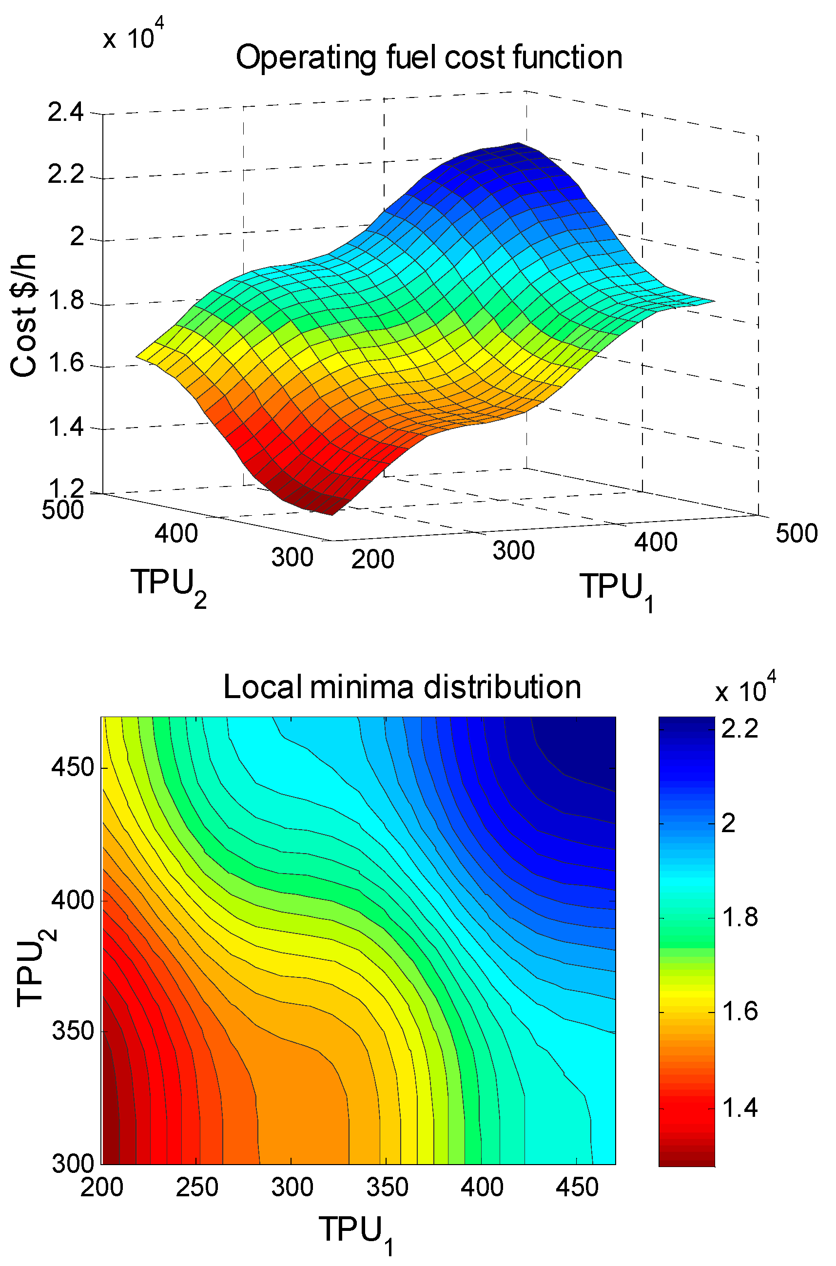
4.3. Illustrative Example

Two practical operating power limitations, VPL effects and RRLs, are considered for TPU operation. In order to demonstrate the effects of VPL and RRLs on the OFC function, the following illustrative examples with two online TPUs, namely, TPU₁ and TPU₂, are considered. The parameters of both TPUs are provided in

Table 1. Thermal power unit (TPU)₁ and TPU₂ power generating system (PGS) parameters.

TPUi	${\mathit{a}}_{\mathit{i}}$	${\mathit{b}}_{\mathit{i}}$	${\mathit{c}}_{\mathit{i}}$	${\mathit{e}}_{\mathit{i}}$	${\mathit{f}}_{\mathit{i}}$	${\mathit{P}}_{\mathit{i}}^{\mathit{m}\mathit{i}\mathit{n}}$	${\mathit{P}}_{\mathit{i}}^{\mathit{m}\mathit{a}\mathit{x}}$	$\mathit{U}{\mathit{R}}_{\mathit{i}}$	$\mathit{D}{\mathit{R}}_{\mathit{i}}$
TPU1	0.00043	21.60	958.29	450	0.041	150	470	80	80
TPU2	0.00063	21.05	1313.60	600	0.036	135	460	80	80

. They are two steam turbine synchronous generators (STSGs) with several valves. In practice, the valves of the STSGs govern the steam throughout isolated nozzle groups. Every group supplies optimum efficiency when working at maximum active output power. Thus, after the real power of the STSG increases, the valves are opened and closed automatically, allowing for the highest efficiency of the STSG (maximum real power delivered) to be obtained. Subsequently, this procedure causes ripple-like effects. Thus, multiple modes with various local minimum are produced by the sinusoidal functions, as shown in Equation (3). The OFC function becomes a high-order of nonlinearity characteristics, as shown in Equation (3).

Moreover, under the effect of RRLs, the real power of a TPU is constrained by $P_i^{min}$ and $P_i^{max}$, as shown in Equation (7), for the purpose of stable operation of an online TPU. This procedure prevents redundant thermal pressure on the combustion equipment and boiler. Thus, the real power range of an online TPU operation is constrained by its corresponding RRLs. The MG-PSO algorithm is used to solve Equations (1)–(7) simultaneously in order to find the new generation limits of the TPU₁ and TPU₂.

Table 1 shows the minimum and maximum real power of TPU₁, $P_1^{min}$ = 150 MW and $P_1^{max}$ = 470 MW, respectively. The minimum and maximum real power of TPU₂ are $P_2^{min}$ = 135 MW and $P_2^{max}$ = 460 MW, respectively. Due to the RRLs limitations, $U{R}_1$= 80 MW/h and $D{R}_1$= 80 MW/h for TPU₁, and $U{R}_2$= 80 MW/h and $D{R}_2$= 80 MW/h for TPU₂ (in our case studies, 1 h). By applying Equations (1)–(7), the new generation limits are $P_1^{min}$ = 200 MW and $P_1^{max}$ = 455 MW for TPU₁ and $P_2^{min}$ = 300 MW and $P_2^{max}$ = 460 MW for TPU₂, respectively. Thus, the generating power of the two TPUs is restricted by their RRLs.

Figure 1 shows the effects of VPL on the total OFC of TPU₁ and TPU₂ with new generation limits due to the RRLs. From the local minima distribution in Figure 1, one can see that multiple modes with local minima are shown in the dark red and blue areas. The economic dispatch of real power and optimum feasible area of TPU₁ become 200 and 455 MW, and those of TPU₂ become 300 and 460 MW, respectively. However, with large-scale TPUs (e.g., more than 500) under the effects of VPL and RRLs, finding the economic dispatch of real power becomes a complex problem.

5. Case Studies and Simulation Results

Four case studies with five PGSs with a medium to a very large number of TPUs were tested to evaluate and measure the MG-PSO algorithm performance, as shown in this section.

(1)

Case study #1: 10-TPU PGS without/with consideration of $P_{l,t}$. This case study has 240 (24 × 10) decision variables.

(2)

Case study #2: 100-TPU PGS by repeating the PGS of case study #1 10 times. This case study has 2400 (24 × 100) decision variables.

(3)

Case study #3: 500-TPU PGS by repeating the PGS of case study #1 50 times. This case study has 12,000 (24 × 500) decision variables.

(4)

Case study #4: 1000-TPU PGS by repeating the PGS of case study #1 500 times. This case study has 24,000 (24 × 1000) decision variables.

In all various PGSs, the VPL effects and RRLs were considered. One day (24 h) was selected with a period of $T$.

Table 2. Daily load demands for case study #1.

t	1	2	3	4	5	6	7	8	9	10	11	12
${\mathit{P}}_{\mathit{d},\mathit{t}}$	1036	1110	1258	1406	1480	1628	1702	1776	1924	2072	2146	2220
t	13	14	15	16	17	18	19	20	21	22	23	24
${\mathit{P}}_{\mathit{d},\mathit{t}}$	2072	1924	1776	1554	1480	1628	1776	2072	1924	1628	1332	1184

shows the daily load demand for case study #1. The daily load demands of the other cases were obtained by multiplying the $N_{gen}/10$ of the corresponding demands of case study #1. MATLAB programming language was used for MG-PSO algorithm. The specifications of the computer are Intel (R) Core (TM), 2 Duo CPU T6570 @ 2.1 GHz, and 4 GB of RAM, Windows 7 Home, 64-bit operating system (for all PGS case studies).

5.1. Performance and Fitness Measures

The performance and fitness measure values shown below were considered to determine the accuracy, consistency, and robustness of various NTOTs in order to solve the DED of real power with the following steps:

(1)

Every NTOT is employed with $N_{run}$ independent runs;

(2)

Every NTOT is employed with $N_{iter}$ iterations;

(3)

The$ensemble averge \mathrm{OFC} \left(F_{cost}\right)$ values in USD were determined by Equation (1) under its real power limitations Equations (4) to (9) over $N_{run}$ independent runs at every t iteration;

(4)

$F_{cost, minimum}$ is the $minimum of optimized \mathrm{OFC}$ values in USD over $N_{run}$ independent runs;

(5)

$F_{cost,maximum}$ is the $maximum of optimized \mathrm{OFC}$ values in USD over $N_{run}$ independent runs;

(6)

$F_{cost,average}$ is the $average of optimized \mathrm{OFC}$ values in USD over $N_{run}$ independent runs;

(7)

$\sigma$ is the $standard deviation of optimized \mathrm{OFC}$ values in USD over $N_{run}$ independent runs;

(8)

The $average time consumed \left(T_{consumed}\right)$ is determined by the overall time implemented by the NTOT after a convergence over $N_{run}$ independent runs.

5.2. Case Study #1: 10-TPU PGS without/with Consideration of Transmission Network Loss

The first PGS consisted of 10 TPUs with the consideration of the VPL effects and RRLs.

Table 3. Data specifications for the 10-TPU PGS (case study #1).

TPUi	1	2	3	4	5	6	7	8	9	10
${\mathit{a}}_{\mathit{i}}$	0.00043	0.00063	0.00039	0.00070	0.00079	0.00056	0.00211	0.00480	0.10908	0.00951
${\mathit{b}}_{\mathit{i}}$	21.60	21.05	20.81	23.90	21.62	17.87	16.51	23.23	19.58	22.54
${\mathit{c}}_{\mathit{i}}$	958.20	1313.6	604.97	471.60	480.29	601.75	502.70	639.40	455.60	692.40
${\mathit{e}}_{\mathit{i}}$	450	600	320	260	280	310	300	340	270	380
${\mathit{f}}_{\mathit{i}}$	0.041	0.036	0.028	0.052	0.063	0.048	0.086	0.082	0.098	0.094
${\mathit{P}}_{\mathit{i}}^{\mathit{m}\mathit{a}\mathit{x}}$	470	460	340	300	243	160	130	120	80	55
${\mathit{P}}_{\mathit{i}}^{\mathit{m}\mathit{i}\mathit{n}}$	150	135	73	60	73	57	20	47	20	55
$\mathit{D}{\mathit{R}}_{\mathit{i}}$	80	80	80	50	50	50	30	30	30	30
$\mathit{U}{\mathit{R}}_{\mathit{i}}$	80	80	80	50	50	50	30	30	30	30

presents $P_{d,t}$ for 24 h for this case study #1. The $P_{l,t}$ was not considered for a fair comparison with other NTOTs. The TPU data were provided by [52]. Table 3 contains the values of RRLs of individual TPUs used in all analyses described in Section 5. Based on these details shown in Table 3 [52], the RRLs range was assumed to be from 0.28% to 0.91% of $P_i^{max}$. The reason for choosing this is because the real power spinning reserve of each TPU is not included in this study. However, the RRLs range is usually in a range of from 2% to 6% of $P_i^{max}$ under the application of a real power spinning reserve of TPU.

Table 4. Parameters utilized in the MG-PSO algorithm for the 10-TPU PGS (case study #1).

Parameters	Exploration Stage		Exploitation Stage
	$\mathit{k}=1$	$\mathit{k}=2$	$\mathit{k}=3$
$\mathit{\gamma }$	0.3	0.3	0.3
c1, c2	2.05	2.05	2.05
${\mathit{N}}_{\mathit{i}\mathit{t}\mathit{e}\mathit{r}}$	150	150	350
${\mathit{w}}_{\mathit{i}\mathit{n}\mathit{i},\mathit{k}}$	0.80	0.80	0.35
${\mathit{w}}_{\mathit{f}\mathit{i}\mathit{n},\mathit{k}}$	0.10	0.20	0.20
$\mathit{g}\mathit{r}\mathit{a}{\mathit{d}}_{\mathit{k}}$	−4.66 × 10−3	−3.99 × 10−3	−4.28 × 10−4

illustrates the specific parameters used in the MG-PSO algorithm for the five PGSs in this research study. It was run with $M=20$, $d=10$, $N_{run}=25$, $N_{iter}=500$, and $N_{grad}=3$ ($N_{grad}=2$ for the exploration stage and $N_{grad}=1$ for the exploitation stage).

Table 5. Minimum real power dispatch results achieved by the MG-PSO algorithm for the 10-TPU PGS without consideration of transmission network loss (case study #1).

t	${\mathit{P}}_{1,\mathit{t}}$	${\mathit{P}}_{2,\mathit{t}}$	${\mathit{P}}_{3,\mathit{t}}$	${\mathit{P}}_{4,\mathit{t}}$	${\mathit{P}}_{5,\mathit{t}}$	${\mathit{P}}_{6,\mathit{t}}$	${\mathit{P}}_{7,\mathit{t}}$	${\mathit{P}}_{8,\mathit{t}}$	${\mathit{P}}_{9,\mathit{t}}$	${\mathit{P}}_{10,\mathit{t}}$	${\mathit{F}}_{\mathit{c}\mathit{o}\mathit{s}\mathit{t},\mathit{m}\mathit{i}\mathit{n}\mathit{i}\mathit{m}\mathit{u}\mathit{m}}$	${\mathit{T}}_{\mathit{c}\mathit{o}\mathit{n}\mathit{s}\mathit{u}\mathit{m}\mathit{e}\mathit{d}}$
1	150.02	135.00	194.93	60.00	122.00	122.96	129.00	47.00	20.04	55.00	28,184.9284	9.23
2	150.02	135.05	268.96	60.05	122.02	122.85	129.00	47.00	20.00	55.00	29,738.3371	9.12
3	226.62	215.00	309.57	60.00	73.01	122.53	129.00	47.24	20.00	55.00	32,884.0400	9.21
4	303.02	222.03	324.00	60.75	122.37	122.81	129.00	47.00	20.00	55.00	36,118.9614	9.23
5	379.42	302.00	291.00	60.04	73.17	122.59	129.65	47.00	20.10	55.00	37,738.0667	9.47
6	456.00	309.17	306.48	60.44	122.12	122.76	129.00	47.00	20.00	55.00	40,942.9400	9.47
7	456.00	309.00	308.99	80.98	172.00	123.99	129.00	47.00	20.00	55.00	42,607.1703	9.72
8	456.00	309.06	309.00	126.99	172.99	152.00	129.00	47.00	20.00	55.00	44,217.7972	9.82
9	456.00	389.00	306.00	176.96	222.04	122.99	129.00	47.00	20.00	55.00	47,653.4300	9.89
10	456.00	396.00	299.00	226.93	222.05	160.99	129.00	77.00	50.00	55.00	51,082.4354	9.16
11	256.01	396.01	341.00	248.76	222.37	160.24	129.58	85.00	52.00	55.00	52,760.8264	9.42
12	456.03	460.00	300.99	298.43	222.53	160.99	129.00	85.00	52.00	55.00	54,507.9729	9.10
13	456.00	396.00	298.00	248.49	222.50	160.00	129.00	85.00	22.00	55.00	51,001.1804	9.36
14	456.76	396.00	287.99	198.88	172.06	122.99	129.28	85.00	20.00	55.00	47,808.6845	9.15
15	379.99	396.00	284.00	180.99	122.99	123.00	129.00	85.00	20.00	55.00	44,544.4962	9.40
16	303.00	316.00	318.00	131.00	74.00	123.00	129.00	85.00	20.00	55.00	39,562.9241	9.20
17	226.00	310.00	288.99	120.99	122.00	122.99	129.00	85.00	20.00	55.00	37,930.0339	9.45
18	303.15	309.00	310.00	121.00	172.84	123.00	129.00	85.00	20.00	55.00	41,163.4372	9.80
19	379.01	389.00	301.99	120.98	173.00	123.00	129.00	85.00	20.00	55.00	44,378.0508	9.61
20	457.00	460.00	313.00	171.00	223.00	123.00	130.00	86.00	21.00	56.00	50,781.9900	9.45
21	456.20	396.00	315.99	121.00	222.74	123.00	129.04	85.00	20.00	55.00	47,611.3299	9.54
22	379.81	316.09	275.99	70.99	172.99	122.99	129.09	85.00	20.00	55.00	41,101.1436	9.35
23	303.00	236.00	197.00	61.00	123.00	123.00	129.00	85.00	20.00	55.00	34,693.3884	9.31
24	226.90	222.44	189.93	60.14	73.00	122.13	129.00	85.00	20.00	55.10	31,476.8566	9.34
Total											1,010,490.42 USD	225.80 s

presents the minimum real power dispatch values of each online TPU at each $t$period over 24 h, i.e., $P_{i,t}=1, 2, \dots , 10$, $t=1, 2, \dots , 24$. In addition, Table 5 illustrates $F_{cost,minimum}=\mathrm{USD} \mathrm{1,010,490.42}$, which was obtained from the best run of the MG-PSO algorithm over $N_{run}=25$ independent runs at tth interval. The $T_{consumed}$ during the 24 h period was 225.80 s.

Table 6. Fitness measures comparison between the MG-PSO algorithm and eleven non-traditional optimization techniques (NTOTs) for the 10-TPU PGS without consideration of $P_{l,t}$ (case study #1).

No.	NTOTs	${\mathit{F}}_{\mathit{c}\mathit{o}\mathit{s}\mathit{t},\mathit{m}\mathit{i}\mathit{n}\mathit{i}\mathit{m}\mathit{u}\mathit{m}}$	${\mathit{F}}_{\mathit{c}\mathit{o}\mathit{s}\mathit{t},\mathit{m}\mathit{a}\mathit{x}\mathit{i}\mathit{m}\mathit{u}\mathit{m}}$	${\mathit{F}}_{\mathit{c}\mathit{o}\mathit{s}\mathit{t},\mathit{a}\mathit{v}\mathit{e}\mathit{r}\mathit{a}\mathit{g}\mathit{e}}$	σ	${\mathit{T}}_{\mathit{c}\mathit{o}\mathit{n}\mathit{s}\mathit{u}\mathit{m}\mathit{e}\mathit{d}}$
1	EP [9]	1,048,638.00	NA	NA	NA	902.94
2	GPSO-w [10]	1,027,679.00	1,034,340.00	1,031,716.00	NA	NA
3	EAPSO [17]	1,018,510.00	1,019,302.00	1,018,710.00	NA	37.50
4	TLA [18]	1,019,925.00	1,021,118.00	1,020,411.00	NA	2.94
5	ICA [18]	1,018,467.00	1,021,796.00	1,019,291.00	693.487	NA
6	GA [20]	1,033,481.00	1,042,606.00	1,038,014.00	NA	NA
7	ABC [41]	1,021,576.00	1,024,316.00	1,022,686.00	NA	156.18
8	CSO [52]	1,017,660.00	1,019,286.00	1,018,710.00	302.3103	57.66
9	HIGA [54]	1,108,473.00	1,022,284.00	1,019,328.00	NA	211.8
10	CSDE [57]	1,023,432.00	1,027,634.00	1,026,475.00	NA	18.00
11	CDBCO [58]	1,021,500.00	NA	1,024,300.00	NA	40.20
12	MG-PSO	1,010,490.42	1,010,490.47	1,010,490.45	0.0104	225.80

demonstrates the performance and fitness measure values from using the MG-PSO algorithm for the 10-TPUsPGS without consideration of $P_{l,t}$. A total of 25 independent runs were achieved for the identification of $F_{cost,minimum}$, $F_{cost,average}$ and $F_{cost,maximum}$. The $F_{cost,minimum}$, $F_{cost,average}$, and $F_{cost,maximum}$ obtained by the MG-PSO algorithm were USD 1,010,490.44, USD 1,010,490.45 and USD 1,010,490.47, respectively, and $\sigma =\mathrm{USD} 0.0104$. In addition, Table 6 provides a statistic comparison of the various NTOTs. In the 10-TPU PGS without consideration of $P_{l,t}$ case study #1, 12 NTOTs, namely, the MG-PSO algorithm, the EP algorithm [9], the GPSO-w algorithm [10], the EAPSO algorithm [17], the ICA [18], the TLA [18], the GA [20], the ABC algorithm [41], the CSO algorithm [52], the HIGA [54], the CSDE algorithm [57], and the CDBCO algorithm [58], were applied for comparison. The best statistical results are shown in bold. The MG-PSO algorithm significantly outperformed the other 11 competitive NTOTs, as shown in Table 6, and obtained better solutions than the other 11 NTOTs in terms of $F_{cost,minimum}$, $F_{cost,average}$, and $F_{cost,maximum}$. Although the MG-PSO algorithm consumed more time than the other NTOTs shown in Table 6, such as the TLA [18] and the CSDE algorithm [57], it displayed a better convergence of rate, consistency, and accuracy of obtaining the best and accurate solution, $\sigma =\mathrm{USD} 0.0104$. The outcomes in Table 5 and Table 6 indicate that this algorithm is robust, accurate, stable, and can obtain the best solution with consistent results.

Figure 2A depicts the convergence characteristic of this algorithm for case study #1, and Figure 2B shows the best (minimum) OFC distribution over 25 independent runs. At every iteration, the $F_{cost}$ values were obtained from 25 independent runs over 24 periods (each t period is 1 h). The MG-PSO algorithm stabilized at approximately 220 iterations and attained $F_{cost,average}$ of approximately USD 1,010,490, as shown in Figure 2A. Hence, this algorithm efficiently and effectively converged to the optimum solution.

Figure 2B depicts the deviation of the minimized $F_{cost}$ over 25 independent runs obtained by this algorithm for the 10-TPU PGS without consideration of $P_{l,t}$ case study #1. The minimized $F_{cost}$ diverged between USD 1,010,490.47 and USD 1,010,490.44, indicating that this algorithm can provide a reliable solution and consistent outcomes. Thus, the MG-PSO algorithm can solve the DED of the 10-TPU PGS under VPL effects and RRLs without consideration of transmission power loss.

Figure 3A shows the real power generation $P_{i,t}, i=1, 2, \dots , 10, \mathrm{and} t=1, 2, \dots , 24,$ delivered by the 10-TPU PGS without consideration of $P_{l,t}$ over 24 h when using the MG-PSO algorithm. The generating powers of TPU₁, TPU₂, TPU₄, and TPU₅ changed mainly during the day to meet the load demand, whereas the generating powers of TPU₃, TPU₆, TPU₇, TPU₈, TPU₉, and TPU₁₀ gradually changed.

Table 7. Load demand and real power delivered for the 10-TPU PGS without consideration of $P_{l,t}$ (case study #1).

t	1	2	3	4	5	6	7	8	9	10	11	12
${\mathit{P}}_{\mathit{d},\mathit{t}}$	1036	1110	1258	1406	1480	1628	1702	1766	1924	2072	2146	2220
${\mathit{P}}_{\mathit{i},\mathit{t}}$	1035.95	1109.95	1257.97	1405.98	1479.97	1627.97	1701.96	1777.04	1923.99	2017.97	2145.97	2219.97
t	13	14	15	16	17	18	19	20	21	22	23	24
${\mathit{P}}_{\mathit{d},\mathit{t}}$	2072	1924	1776	1554	1480	1628	1776	2072	1924	1628	1332	1184
${\mathit{P}}_{\mathit{i},\mathit{t}}$	2171.99	1923.96	1775.97	1554.00	1479.97	1627.99	1775.98	2071.76	1923.97	1627.95	1332.00	1183.64

shows the load demand $P_{d,t}$ and the generation estimated $P_{i,t}, i=1, 2, \dots ,10, t=1, 2, \dots , 24,$ by MG-PSO algorithm during the day. This PGS capacity was 40,108 MW for the 24 h period (the sum of $P_{d,t}$ individuals during the day (40,108 MWh)); it is of a medium size with 10 TPUs. The maximum demand was 2220 MW at $t=12,$ and the minimum demand was is 1036 MW at $t=1$.

Figure 4A shows this algorithm’s capability in estimating the generation of all 10 TPUs during the day. The outcomes from Table 7 and Figure 4A demonstrate that the MG-PSO algorithm is stable, consistent, and able to estimate the required generation for 10 TPUs without consideration of transmission network loss during the day.

The second PGS also has 10 TPUs, and the data specifications of this power system are available in Table 3. The VPL effects, RRLs, and the transmission network loss at each period t, $P_{l,t}, t=1, 2, \dots , 24,$ were considered.

Table 8. Loss coefficients (B-matrix) for the 10-TPU PGS (1 × 10⁻⁵).

Bji	1	2	3	4	5	6	7	8	9	10
1	8.70	0.43	−4.61	0.36	0.32	−0.66	0.96	−1.60	0.80	−0.10
2	0.43	8.30	−0.97	0.22	0.75	−0.28	5.04	1.70	0.54	7.20
3	−4.61	−0.97	9.00	−2.00	0.63	3.00	1.70	−4.30	3.10	−2.00
4	0.36	0.22	−2.00	5.30	0.47	2.62	−1.96	2.10	0.67	1.80
5	0.32	0.75	0.63	0.47	8.60	−0.80	0.37	0.72	−0.90	0.69
6	−0.66	−0.28	3.00	2.62	−0.80	11.80	−4.90	0.30	3.00	−3.00
7	0.96	5.04	1.70	−1.96	0.37	−4.90	8.24	−0.90	5.90	−0.60
8	−1.60	1.70	−4.30	2.10	0.72	0.30	−0.90	1.20	−0.96	0.56
9	0.80	0.54	3.10	0.67	−0.90	3.00	5.90	−0.96	0.93	−0.30
10	−0.10	7.20	−2.00	1.80	0.69	−3.00	−0.60	0.56	−0.30	0.99

presents the B-matrix loss coefficients [15] of this PGS, and the parameters utilized in MG-PSO algorithm are shown in Table 4.

Table 9. Minimum real power dispatch results achieved by the MG-PSO algorithm for the 10-TPU PGS with consideration of the transmission network loss (case study #1).

t	${\mathit{P}}_{1,\mathit{t}}$	${\mathit{P}}_{2,\mathit{t}}$	${\mathit{P}}_{3,\mathit{t}}$	${\mathit{P}}_{4,\mathit{t}}$	${\mathit{P}}_{5,\mathit{t}}$	${\mathit{P}}_{6,\mathit{t}}$	${\mathit{P}}_{7,\mathit{t}}$	${\mathit{P}}_{8,\mathit{t}}$	${\mathit{P}}_{9,\mathit{t}}$	${\mathit{P}}_{10,\mathit{t}}$	${\displaystyle \sum }_{\mathit{i}=1 }^{10}{\mathit{P}}_{\mathit{i}}$	Pl,t	${\mathit{P}}_{\mathit{d},\mathit{t}}$	$\Delta {\mathit{P}}_{\mathit{t}}$	${\mathit{F}}_{\mathit{c}\mathit{o}\mathit{s}\mathit{t},\mathit{m}\mathit{i}\mathit{n}\mathit{i}\mathit{m}\mathit{u}\mathit{m}}$	${\mathit{T}}_{\mathit{c}\mathit{o}\mathit{n}\mathit{s}\mathit{u}\mathit{m}\mathit{e}\mathit{d}}$
1	150.00	135.00	207.00	60.12	122.00	122.99	129.0	47.00	20.00	55.00	1048.12	12.12	1036	0.00	28,439.90	9.46
2	150.21	135.01	282.54	60.99	122.01	122.87	129.0	47.00	20.00	55.00	1124.63	14.63	1110	0.00	30,060.63	9.22
3	226.11	135.00	308.00	60.35	172.42	123.00	129.0	47.00	20.00	55.00	1275.88	17.88	1258	0.00	33,338.67	9.31
4	303.00	215.00	305.00	60.20	172.21	122.95	129.0	47.00	20.00	55.00	1429.36	23.37	1406	0.00	36,637.72	9.33
5	379.81	222.21	297.63	60.00	172.71	122.42	129.5	47.00	20.00	55.00	1506.28	26.28	1480	0.00	38,296.74	9.57
6	456.50	222.20	305.04	80.06	222.61	122.56	129.5	47.00	20.00	55.00	1660.47	32.47	1628	0.00	41,715.72	9.57
7	456.50	302.27	312.27	120.41	172.70	122.41	129.5	47.00	20.00	55.00	1738.06	36.06	1702	0.00	43,450.29	9.82
8	456.50	309.27	299.55	170.45	172.70	122.61	129.52	77.00	20.00	55.00	1812.60	36.60	1776	0.00	45,261.46	9.92
9	456.50	389.50	299.57	189.50	222.61	122.43	129.5	85.30	20.00	55.00	1969.90	45.90	1924	0.00	48,733.35	9.69
10	456.50	396.80	325.60	239.50	222.91	160.00	129.5	115.30	20.00	55.00	2121.11	49.11	2072	0.00	52,202.09	9.26
11	458.40	396.80	340.15	289.50	227.60	160.02	129.5	120.00	20.00	55.00	2196.97	50.97	2146	0.00	53,836.89	9.52
12	456.50	460.00	325.14	300.00	222.61	160.00	129.5	120.00	50.00	55.00	2278.75	58.75	2220	0.00	55,806.50	9.19
13	456.50	396.80	298.55	300.00	222.60	122.42	129.5	120.00	20.00	55.00	2121.36	49.36	2072	0.00	52,386.68	9.39
14	456.50	316.80	302.45	250.00	222.60	122.40	129.5	90.00	20.00	55.00	1965.25	41.25	1924	0.00	48,807.00	9.25
15	379.80	309.50	294.85	241.12	172.76	122.46	129.5	85.30	20.00	55.00	1810.28	34.28	1776	0.00	45,390.70	9.49
16	303.25	229.50	318.48	191.24	122.83	122.40	129.5	85.30	20.01	55.00	1577.50	23.50	1554	0.00	40,201.11	9.28
17	226.60	222.20	287.67	180.76	172.70	122.68	129.50	85.30	20.00	55.00	1502.41	22.41	1480	0.00	38,564.89	9.55
18	303.25	222.20	312.74	180.80	222.60	123.52	129.50	85.30	20.00	55.00	1654.90	26.90	1628	0.00	41,874.71	9.89
19	379.80	302.20	313.17	180.80	222.60	122.56	129.50	85.30	20.00	55.00	1810.92	34.92	1776	0.00	45,252.41	9.70
20	456.50	382.20	340.17	230.81	230.40	160.01	129.50	115.30	20.00	55.00	2119.89	47.89	2072	0.00	52,004.90	9.51
21	456.50	396.90	301.41	180.80	222.60	122.40	129.50	85.30	20.00	55.00	1970.40	46.40	1924	0.00	48,721.06	9.54
22	379.80	316.80	278.34	130.83	172.70	122.62	129.50	55.30	20.00	55.00	1660.89	32.89	1628	0.00	41,817.63	9.45
23	303.20	236.80	198.30	118.30	122.80	122.40	129.96	47.00	20.00	55.00	1353.76	21.76	1332	0.00	35,306.36	9.39
24	226.60	222.20	184.72	120.40	73.01	122.50	129.50	47.00	20.00	55.00	1200.92	16.92	1184	0.00	31,853.95	9.39
Total												802.62 MW			1,029,961.36 USD	227.7 s

exhibits the minimum real power values of each TPU at each t period for 24 h. In addition, $F_{cost,minimum}=\mathrm{USD} \mathrm{1,029,961.36}$ is shown in Table 9, which was obtained from the MG-PSO algorithm’s best run over 25 independent runs during the 24 h period. Table 9 also presents $\Delta P_t=0.0 \mathrm{MW}$ and total $P_{l,t}=802.62 \mathrm{MW}$(sum of $P_{l,t}$individuals during the 24 h period). The sum of $P_{l,t}$ individuals provides details about the optimum power loss in each period and the volume of energy loss during the day (802.62 MWh). Table 9 shows $T_{consumed}=227.7 \mathrm{s}$ in the 24 h period.

Table 10. Fitness measure comparison between the MG-PSO algorithm and nine NTOTs for the 10-TPU PGS with consideration of $P_{l,t}$ (case study #1).

No.	NTOTS	${\mathit{F}}_{\mathit{m}\mathit{i}\mathit{n}\mathit{i}\mathit{m}\mathit{u}\mathit{m}}$	${\mathit{F}}_{\mathit{m}\mathit{a}\mathit{x}\mathit{i}\mathit{m}\mathit{u}\mathit{m}}$	${\mathit{F}}_{\mathit{a}\mathit{v}\mathit{e}\mathit{r}\mathit{a}\mathit{g}\mathit{e}}$	σ	${\mathit{P}}_{\mathit{l},\mathit{t}}$	${\mathit{T}}_{\mathit{c}\mathit{o}\mathit{n}\mathit{s}\mathit{u}\mathit{m}\mathit{e}\mathit{d}}$
1	AIS [10]	1,045,715.00	1,048,431.00	1,047,050.00	NA	835.62	1858.20
2	GA [10]	1,052,251.00	1,062,511.00	1,058,041.00	NA	NA	206.64
3	GPSO-w [10]	1,048,410.00	1,057,170.00	1,052,092.00	NA	NA	245.58
4	CDBCO [14]	1,042,900.00	1,043,626.00	1,044,700.00	NA	839.31	91.80
5	ICA [16]	1,040,758.00	1,043,173.00	1,041,664.00	603.758	848.79	NA
6	CSO [52]	1,038,320.00	1,042,518.00	1,039,374.00	395.673	802.68	88.86
7	EBSO [53]	1,038,915.00	1,039,272.00	1,039,188.00	NA	NA	13.20
8	HIGA [54]	1,041,088.00	1,042,516.00	1,041,218.00	NA	853.53	NA
9	ECE [71]	1,043,989.00	NA	1,044,470.00	NA	NA	228.0
10	MG-PSO	1,029,961.36	1,029,961.40	1,029,961.37	0.035	802.62	227.7

present the fitness values obtained with the MG-PSO algorithm for the 10-TPU PGS with the consideration of $P_{l,t}$. Table 10 shows the 10 NTOTs, namely, the MG-PSO algorithm, the AIS algorithm [10], the GA [10], the GPSO-w algorithm [10], the CDBCO algorithm [14], the ICA [16], the CSO algorithm [52], the EBSO algorithm [53], the HIGA [54], and the ECE algorithm [71], that were used for comparison. The best outcomes are shown in bold. The $F_{cost,minimum}$, $F_{cost,average}$, and $F_{cost,maximum}$ obtained by the MG-PSO algorithm were USD 1,029,961.31, USD 1,029,961.37 and USD 1,029,961.40, respectively. The MG-PSO algorithm outperformed all other NTOTs regardless of $F_{cost,minimum}$, $F_{cost,average}$, and $F_{cost,maximum}$. Although the MG-PSO algorithm consumed more time than the other NTOTs, such as the EBSO algorithm [53], it showed better performance in the rate of convergence and accuracy of the solution $\sigma =\mathrm{USD} 0.035$. The outcomes shown in Table 9 and Table 10 indicate that this algorithm is robust and stable and obtains the solution with consistent results. Furthermore, it provided the balance of real power constraint at each t period, which was computed by Equation (8), at each t period $\Delta P_t=0.0$, which means that the real power balance constraint of 10-TPU PGS was efficiently achieved. Moreover, the sum of individuals, $P_{l,t}=802.62 \mathrm{MW}$, during the 24 h period is less than the values demonstrated in Table 10.

Figure 2C depicts this algorithm’s convergence characteristics, and Figure 2D plots the minimum OFCs distribution over 25 independent runs. The $F_{cost}$ values at each $t$iteration were obtained from 25 independent runs in 24 h. The MG-PSO algorithm settled approximately at $t=230$ s and realized $F_{cost,average }=\mathrm{USD}\mathrm{1,029,961}$. Thus, this algorithm efficiently and effectively converged to the minimum solution.

Figure 2D shows the minimum $F_{cost}$deviation over 25 independent runs. The minimized $F_{cost}$diverged between USD 1,029,961.40 and USD 1,029,961.31, indicating that this algorithm can provide a reliable solution and consistent results. Thus, the MG-PSO algorithm can solve the DED of 10 TPU under VPL effects and RRLs with transmission network loss.

Figure 3B shows the real power generation $(P_{i,t}) \mathrm{where} i=1, 2, \dots , 10, \mathrm{and} t=1, 2, \dots , 24,$ delivered by the 10 TPUs during the period of a day using the MG-PSO algorithm. The generating power of TPU₁, TPU₂, and TPU₅ primarily changed during the day to meet the load demand whereas the generating power of TPU₃, TPU₄, TPU₆, TPU₇, TPU₈, TPU₉, and TPU₁₀ gradually changed during the day.

Figure 4B shows this algorithm’s capability to estimate the generation of all 10 TPUs during the day. The minimum and maximum load demands were 2220 and 1036 MW, respectively. The sum load demand during the 24 h period was 40,108 MW. The MG-PSO algorithm was applied to estimate the system generation of case study #1, and the sum of the 24 h period was $P_{i,t}=$ 40,910.62 MW (the sum of $P_{i,t}$ individuals provided details about the optimum power generation in each period and the energy generation volume during the day (40,910.62 MWh)). The MG-PSO algorithm can meet the load demands at any time during the day. The difference between $P_{i,t}$ and $P_{l,t}$ in each one hour shown in Figure 4B is the transmission network loss $P_{l,t}$.

The MG-PSO algorithm is stable and consistent in solving the DED problem for 10 TPUs with RRLs and VPL effects, including transmission network loss (case study #1).

These outcomes provide technical details for economic dispatch operators to identify which a group of TPUs is subjected to the maximum burden during the 24 h period in order to maintain the stability and reliability of a PGS in the case of a sudden change in the load demand or generation fault or/and, and they also enable them to schedule the period maintenance of TPUs.

5.3. Case Studies #2 to #4: 100-, 500-, and 1000-TPU PGS

Most NTOTs available in the literature have focused on finding the solution to the DED problem with 10-TPU PGS (d = 10) under VPL effects and RRLs. These NTOTs can solve such a complex problem. However, in the DED problem, when very large-scale TPUs under VPL effects and RRLs are used, few NTOTs are applied. The MG-PSO algorithm was utilized in case studies #2 to #4 (three large-scale DED problems). They comprise 100, 500, and 1000 TPUs by duplicating case study #1 (10-TPU PGS) by 10, 50, and 100 times, respectively.

The number of variables, i.e., real power values of online TPUs in the period of 24 h, increased from 240 decision variables to 2400, 12,000, and 24,000, respectively.

Using many TPUs with VPL effects and RRLs introduces difficulty and complexity in the solution to the real power DED problem because of numerous inequality power limitations that cause multiple modes and local minima.

Table 11. Parameters utilized in the MG-PSO algorithm for the 100-, 500-, and 1000-TPU PGS.

Parameters	Exploration Stage			Exploitation Stage
	$\mathit{k}=1$	$\mathit{k}=2$	$\mathit{k}=3$	$\mathit{k}=4$
$\mathit{\gamma }$	0.3	0.3	0.3	0.3
c1, c2	2.05	2.05	2.05	2.05
${\mathit{N}}_{\mathit{i}\mathit{t}\mathit{e}\mathit{r}}$	150	150	150	350
${\mathit{w}}_{\mathit{i}\mathit{n}\mathit{i},\mathit{k}}$	0.90	0.80	0.80	0.35
${\mathit{w}}_{\mathit{f}\mathit{i}\mathit{n},\mathit{k}}$	0.05	0.10	0.20	0.20
$\mathit{g}\mathit{r}\mathit{a}{\mathit{d}}_{\mathit{k}}$	−5.66 × 10−3	−4.66 × 10−3	−3.99 × 10−3	−4.28 × 10−4

shows the parameters used in the MG-PSO algorithm. It was run with $M=20,d=100,500,\mathrm{and}1000,N_{iter}=500,N_{run}=25,\mathrm{and}{N}_{grad}=4,$ (three used in the exploration stage and one in the exploitation stage) through trial and error due to the problem complexity, as shown in Table 11.

For the 100-TPU PGS in case study #2, the outcomes of the CSO [52], GA [55], GPSO-w [55], FA [55], and SAFA [55] were compared with the results obtained by the MG-PSO algorithm over 25 independent runs, and these results are displayed in

Table 12. Fitness measure comparison between the MG-PSO algorithm and different NTOTs for case studies #2 to #4.

No.	NTOTs	${\mathit{F}}_{\mathit{c}\mathit{o}\mathit{s}\mathit{t},\mathit{m}\mathit{i}\mathit{n}\mathit{i}\mathit{m}\mathit{u}\mathit{m}}$	${\mathit{F}}_{\mathit{c}\mathit{o}\mathit{s}\mathit{t},\mathit{m}\mathit{a}\mathit{x}\mathit{i}\mathit{m}\mathit{u}\mathit{m}}$	${\mathit{F}}_{\mathit{c}\mathit{o}\mathit{s}\mathit{t},\mathit{a}\mathit{v}\mathit{e}\mathit{r}\mathit{a}\mathit{g}\mathit{e}}$	σ	${\mathit{T}}_{\mathit{c}\mathit{o}\mathit{n}\mathit{s}\mathit{u}\mathit{m}\mathit{e}\mathit{d}}$
Case #3: 100 TPU
1	CSO [52]	10,183,633.00	10,192,352.00	10,185,287.00	1323.00	297.00
2	GA [55]	10,908.741.00	11,987,675.00	11,584,628.00	NA	542.40
3	GPSO-w [55]	10,366.076.00	11,310,279.00	10,766,385.00	NA	353.40
4	FA [55]	10,197,269.00	11,216,243.00	10,419,457.00	NA	266.46
5	SAFA [55]	10,183,819.00	10,388,958.00	10,286,043.00	NA	84.60
6	MG-PSO	9,549,134.75	9,549,134.96	9,549,134.68	0.098	419.98
Case #4: 500 TPU
1	CSO [52]	51.044,611.00	51,082,986.00	51,050,457.00	6067.00	534.60
2	MG-PSO	49,655,500.34	49,655,501.81	49,655,501.73	0.511	765.29
Case #5: 1000 TPU
1	CSO [52]	102,122,060.00	102,186,925.00	102,133,104.00	9627.00	721.8
2	MG-PSO	99,311,000.68	99,311,003.63	99,311.001.47	1.022	903.34

. The MG-PSO algorithm has a vast advantage over its competitive optimization techniques in terms of $F_{cost,minimum}$, $F_{cost,average}$, and $F_{cost,maximum}$. A small $\mathsf{\sigma }$ indicates that improved performance is achieved by the MG-PSO algorithm for the balance convergence rate and solution accuracy.

For case studies #3 and # 4 with 500 and 1000 TPUs, only the CSO [52] algorithm was compared with the MG-PSO algorithm, as shown in Table 12. Table 12 displays that the outcomes of the fitness measures values and σ of the MG-PSO algorithm were the best.

Figure 5A,C,E depict the MG-PSO algorithm’s convergence characteristics, and Figure 5B,D,F illustrate the minimum OFCs distribution over 25 independent runs for case studies #2 to #4. The optimum dispatch outcomes are not provided due to reasons regarding length, that is, as the $N_{gen}$ increases, the total OFC grows linearly, and the problem becomes complicated.

Figure 5A,C,E depict the convergence characteristics obtained by the MG-PSO algorithm in three case studies; this algorithm only takes approximately 400 iterations to reach the optimized OFC. In addition, it can smoothly converge to the optimum value without any fluctuations, even for the DED of real power problems of 500 and 1000 TPUs. This feature proves that the MG-PSO algorithm has convergence consistency.

Figure 5B,D,F show the $F_{cost,minimum}$ (minimum $F_{cost})$distribution over 25 independent runs for case studies #2 to #4. The $F_{cost,minimum}$ over N_run = 25 diverged in a small range, which means that the MG-PSO algorithm is stable even for a large-scale real power DED problem. This result proves that the MG-PSO algorithm for large-scale TPUs with numerous local minima suffers from varying degrees of premature convergence when distinct negative gradients are used. This variety in using distinct negative gradients helps M particles to steadily move toward the solution, and the particles can prevent the fall within the local minimum. Thus, the MG-PSO algorithm is robust for overcoming dimensionality for the large-scale real power DED problem.

5.4. MG-PSO Algorithm with Several Fitness Measures

The MG-PSO algorithm is efficient in handling different complex real-world problems in science and engineering, including power system problems because of its accuracy in obtaining an optimal solution, reliability, stability and consistency, rate of convergence, and robustness, as shown in Section 5 (5.1–5.6) [50] and other research papers [62,63,64].

6. Conclusions

The MG-PSO algorithm is positively used to cover the lack of non-traditional optimization techniques (NTOTs) in solving the real power limitations in the dynamic economic dispatch of large-scale thermal power units under valve-point loading and ramp-rate limitations. Due to the use of distinct negative gradients by the M particles inside a swarm by seeking a solution in two stages, namely, exploration and exploitation, this integration of both stages provides an equilibrium between the M particles’ local and global search capabilities. The MG-PSO algorithm is applied to evaluate Equations (1)–(9) using 10, 100, 500, and 1000 TPUs for 24 h. The results reveal that the MG-PSO algorithm solved the OFC function and their power limitations and responds to the load demand changes in each time interval during the 24 h period. In addition, the outcomes show that the MG-PSO algorithm not only largely outperforms its competitive algorithm, namely, the GPSO-w, algorithm, but it also provides better real power dispatch outcomes with a lower total OFC than other NTOTs. The NTOTs mostly suffer from premature convergence and dimensionality when numbers increases, e.g., more than 500 in the problem of the real power DED. However, the MG-PSO algorithm is sufficient even for large-scale TPUs. The MG-PSO algorithm performance is compared with various NTOTs, including the GPSO-w algorithm, and its superiority is validated in several fitness performance measures, i.e., accuracy, rate of convergence, stability, and consistency. Thus, it is verified to be a stable, robust, efficient, and consistent, which can solve the DED of real power for large-scale power generating systems (PGSs). The current research study provides essential details for economic dispatch operators to build future PGS operating programs to achieve economic benefits.

References

1. Zhang, Y.; Gong, D.-W.; Geng, N.; Sun, X.-Y. Hybrid bare-bones PSO for dynamic economic dispatch with valve-point effects. Appl. Soft Comput. 2014, 18, 248–260. [Google Scholar] [CrossRef]
2. Lokeshgupta, B.; Sivasubramani, S. Multi-objective dynamic economic and emission dispatch with demand side management. Int. J. Electr. Power Energy Syst. 2018, 97, 334–343. [Google Scholar] [CrossRef]
3. Roy, S. The maximum likelihood optima for an economic load dispatch in presence of demand and generation variability. Energy 2018, 147, 915–923. [Google Scholar] [CrossRef]
4. Mason, K.; Duggan, J.; Howley, E. A multi-objective neural network trained with differential evolution for dynamic economic emission dispatch. Int. J. Electr. Power Energy Syst. 2018, 100, 201–221. [Google Scholar] [CrossRef]
5. Ciornei, I.; Kyriakides, E. Recent methodologies and approaches for the economic dispatch of generation in power systems. Int. Trans. Electr. Energy Syst. 2012, 23, 1002–1027. [Google Scholar] [CrossRef]
6. Niknam, T.; Mojarrad, H.D.; Meymand, H.Z. A new particle swarm optimization for non-convex economic dispatch. Eur. Trans. Electr. Power 2010, 21, 656–679. [Google Scholar] [CrossRef]
7. Alomoush, M.I.; Oweis, Z.B. Environmental-economic dispatch using stochastic fractal search algorithm. Int. Trans. Electr. Energy Syst. 2018, 28, e2530. [Google Scholar] [CrossRef]
8. Yu, X.; Xianrui, Y.X.; Lu, Y. Economic and emission dispatch using ensemble multi-objective differential evolution algorithm. Sustainability 2018, 10, 418. [Google Scholar] [CrossRef] [Green Version]
9. Coelho, L.D.S.; Mariani, V. Correction to “Combining of Chaotic Differential Evolution and Quadratic Programming for Economic Dispatch Optimization with Valve-Point Effect”. IEEE Trans. Power Syst. 2006, 21, 989–996. [Google Scholar]
10. Hemamalini, S.; Simon, S. Dynamic economic dispatch using artificial bee colony algorithm for units with valve-point effect. Eur. Trans. Electr. Power 2011, 21, 70–81. [Google Scholar] [CrossRef]
11. Vo, D.N.; Schegner, P.; Ongsakul, W. Cuckoo search algorithm for non-convex economic dispatch. IET Gener. Transm. Distrib. 2013, 7, 645–654. [Google Scholar] [CrossRef]
12. Singh, D.; Dhillon, J. Ameliorated grey wolf optimization for economic load dispatch problem. Energy 2019, 169, 398–419. [Google Scholar] [CrossRef]
13. Singh, P.; Dwivedi, P. A novel hybrid model based on neural network and multi-objective optimization for effective load forecast. Energy 2019, 182, 606–622. [Google Scholar] [CrossRef]
14. Lu, P.; Zhou, J.; Zhang, H.; Zhang, R.; Wang, C. Chaotic differential bee colony optimization algorithm for dynamic economic dispatch problem with valve-point effects. Int. J. Electr. Power Energy Syst. 2014, 62, 130–143. [Google Scholar] [CrossRef]
15. Elsheakh, Y.; Zou, S.; Ma, Z.; Zhang, B. Decentralised gradient projection method for economic dispatch problem with valve point effect. IET Gener. Transm. Distrib. 2018, 12, 3844–3851. [Google Scholar] [CrossRef]
16. Mohammadi-Ivatloo, B.; Rabiee, A.; Soroudi, A.; Ehsan, M. Imperialist competitive algorithm for solving non-convex dynamic economic power dispatch. Energy 2012, 44, 228–240. [Google Scholar] [CrossRef] [Green Version]
17. Niknam, T.; Golestaneh, F. Enhanced adaptive particle swarm optimisation algorithm for dynamic economic dispatch of units considering valve-point effects and ramp rates. IET Gener. Transm. Distrib. 2012, 6, 424–435. [Google Scholar] [CrossRef]
18. Niknam, T.; Azizipanah-Abarghooee, R.; Aghaei, J. A new modified teaching-learning algorithm for reserve constrained dynamic economic dispatch. IEEE Trans. Power Syst. 2012, 28, 749–763. [Google Scholar] [CrossRef]
19. Zaman, M.F.; Elsayed, S.M.; Ray, T.; Sarker, R.A. Evolutionary Algorithms for Dynamic Economic Dispatch Problems. IEEE Trans. Power Syst. 2016, 31, 1486–1495. [Google Scholar] [CrossRef]
20. Wu, Z.; Ding, J.; Wu, Q.; Jing, Z.; Zheng, J. Reserve constrained dynamic economic dispatch with valve-point effect: A two-stage mixed integer linear programming approach. CSEE J. Power Energy Syst. 2017, 3, 203–211. [Google Scholar] [CrossRef]
21. Wu, H.; Liu, X.; Ding, M. Dynamic economic dispatch of a microgrid: Mathematical models and solution algorithm. Int. J. Electr. Power Energy Syst. 2014, 63, 336–346. [Google Scholar] [CrossRef]
22. Zhu, Y.; Qiao, B.; Dong, Y.; Qu, B.; Wu, D. Multiobjective dynamic economic emission dispatch using evolutionary algorithm based on decomposition. IEEJ Trans. Electr. Electron. Eng. 2019, 14, 1323–1333. [Google Scholar] [CrossRef]
23. Alshammari, M.E.; Ramli, M.A.M.; Mehedi, I.M. An Elitist Multi-Objective Particle Swarm Optimization Algorithm for Sustainable Dynamic Economic Emission Dispatch Integrating Wind Farms. Sustainability 2020, 12, 7253. [Google Scholar] [CrossRef]
24. Somuah, C.B.; Khunaizi, N. Application of linear programming dispatch technique to dynamic generation allocation. IEEE Trans. Power Syst. 1990, 5, 20–26. [Google Scholar] [CrossRef]
25. Lin, C.E.; Viviani, G.L. Hierarchical Economic Dispatch for Piecewise Quadratic Cost Functions. IEEE Trans. Power Appar. Syst. 1984, PAS-103, 1170–1175. [Google Scholar] [CrossRef]
26. Dhar, R.; Mukherjee, P. Reduced-gradient method for economic dispatch. Proc. Inst. Electr. Eng. 1973, 120, 608–610. [Google Scholar] [CrossRef]
27. Binetti, G.; Davoudi, A.; Naso, D.; Turchiano, B.; Lewis, F.L. A Distributed Auction-Based Algorithm for the Nonconvex Economic Dispatch Problem. IEEE Trans. Ind. Inform. 2013, 10, 1124–1132. [Google Scholar] [CrossRef]
28. Hu, F.; Hughes, K.J.; Ingham, D.B.; Ma, L.; Pourkashanian, M. Dynamic economic and emission dispatch model considering wind power under Energy Market Reform: A case study. Int. J. Electr. Power Energy Syst. 2019, 110, 184–196. [Google Scholar] [CrossRef] [Green Version]
29. McLarty, D.; Panossian, N.; Jabbari, F.; Traverso, A. Dynamic economic dispatch using complementary quadratic programming. Energy 2019, 166, 755–764. [Google Scholar] [CrossRef]
30. Mahdi, F.P.; Vasant, P.; Kallimani, V.; Watada, J.; Fai, P.Y.S.; Abdullah-Al-Wadud, M. A holistic review on optimization strategies for combined economic emission dispatch problem. Renew. Sustain. Energy Rev. 2018, 81, 3006–3020. [Google Scholar] [CrossRef]
31. Basu, M. Quasi-oppositional group search optimization for multi-area dynamic economic dispatch. Int. J. Electr. Power Energy Syst. 2016, 78, 356–367. [Google Scholar] [CrossRef]
32. Huang, Y.-X.; Wang, X.-D.; Cheng, C.; Lin, D.T.-W. Geometry optimization of thermoelectric coolers using simplified conjugate-gradient method. Energy 2013, 59, 689–697. [Google Scholar] [CrossRef]
33. Azizipanah-Abarghooee, R.; Niknam, T.; Gharibzadeh, M.; Golestaneh, F. Robust, fast and optimal solution of practical economic dispatch by a new enhanced gra-dient-based simplified swarm optimisation algorithm. IET Gener. Transm. Distrib. 2013, 7, 620–635. [Google Scholar] [CrossRef]
34. Azizipanah-Abarghooee, R.; Dehghanian, P.; Terzija, V. Practical multi-area bi-objective environmental economic dispatch equipped with a hybrid gradient search method and improved Jaya algorithm. IET Gener. Transm. Distrib. 2016, 10, 3580–3596. [Google Scholar] [CrossRef] [Green Version]
35. Hemamalini, S.; Simon, S.P. Dynamic economic dispatch using artificial immune system for units with valve-point effect. Int. J. Electr. Power Energy Syst. 2011, 33, 868–874. [Google Scholar] [CrossRef]
36. Basu, M. Artificial immune system for dynamic economic dispatch. Int. J. Electr. Power Energy Syst. 2011, 33, 131–136. [Google Scholar] [CrossRef]
37. Hatata, A.Y.; Hafez, A.A. Ant lion optimizer versus particle swarm and artificial immune system for economical and eco-friendly power system operation. Int. Trans. Electr. Energy Syst. 2019, 29, e2803. [Google Scholar] [CrossRef]
38. Chao-Lung, C. Improved genetic algorithm for power economic dispatch of units with valve-point effects and multiple fuels. IEEE Trans. Power Syst. 2005, 20, 1690–1699. [Google Scholar]
39. Zou, D.; Li, S.; Kong, X.; Ouyang, H.; Li, Z. Solving the combined heat and power economic dispatch problems by an improved genetic algorithm and a new constraint handling strategy. Appl. Energy 2019, 237, 646–670. [Google Scholar] [CrossRef]
40. Yuan, Y.; Zhang, X.; Ju, P.; Li, Q.; Qian, K.; Fu, Z. Determination of economic dispatch of wind farm-battery energy storage system using Genetic Algorithm. Int. Trans. Electr. Energy Syst. 2014, 24, 264–280. [Google Scholar] [CrossRef]
41. Secui, D.C. A new modified artificial bee colony algorithm for the economic dispatch problem. Energy Convers. Manag. 2015, 89, 43–62. [Google Scholar] [CrossRef]
42. Aydin, D.; Özyön, S.; Yaşar, C.; Liao, T. Artificial bee colony algorithm with dynamic population size to combined economic and emission dis-patch problem. Int. J. Electr. Power Energy Syst. 2014, 54, 144–153. [Google Scholar] [CrossRef]
43. Mahdi, F.P.; Vasant, P.; Watada, J.; Kallimani, V.; Abdullah-Al-Wadud, M. A quantum-inspired particle swarm optimization approach for environmental/economic power dispatch problem using cubic criterion function. Int. Trans. Electr. Energy Syst. 2018, 28, e2497. [Google Scholar] [CrossRef]
44. Tan, Y.; Cao, Y.; Li, C.; Li, Y.; Yu, L.; Zhang, Z.; Tang, S. Microgrid stochastic economic load dispatch based on two-point estimate method and improved particle swarm optimization. Int. Trans. Electr. Energy Syst. 2014, 25, 2144–2164. [Google Scholar] [CrossRef]
45. Elsayed, W.T.; Hegazy, Y.G.; El-Bages, M.S.; Bendary, F.M. Improved Random Drift Particle Swarm Optimization With Self-Adaptive Mechanism for Solving the Power Economic Dispatch Problem. IEEE Trans. Ind. Inform. 2017, 13, 1017–1026. [Google Scholar] [CrossRef]
46. Jadoun, V.K.; Gupta, N.; Niazi, K.; Swarnkar, A. Modulated particle swarm optimization for economic emission dispatch. Int. J. Electr. Power Energy Syst. 2015, 73, 80–88. [Google Scholar] [CrossRef]
47. Shi, Y.; Eberhart, R. A modified particle swarm optimizer. In Proceedings of the 1998 Evolutionary Computation IEEE World Congress on Computational Intelligence, Anchorage, AK, USA, 4–9 May 1998. [Google Scholar]
48. Shi, Y.; Eberhart, R.C. Empirical study of particle swarm optimization. In Proceedings of the Congress on Evolutionary Computation-CEC99, Washington, DC, USA, 6–9 July 1999. [Google Scholar]
49. Al Bahrani, L.T.; Patra, J.C. Orthogonal PSO algorithm for economic dispatch of thermal generating units under various power constraints in smart power grid. Appl. Soft Comput. 2017, 58, 401–426. [Google Scholar] [CrossRef]
50. Al-Bahrani, L.T.; Patra, J.C. Multi-gradient PSO algorithm for optimization of multimodal, discontinuous and non-convex fuel cost function of thermal generating units under various power constraints in smart power grid. Energy 2018, 147, 1070–1091. [Google Scholar] [CrossRef]
51. Elattar, E.E. Environmental economic dispatch with heat optimization in the presence of renewable energy based on modified shuffle frog leaping algorithm. Energy 2019, 171, 256–269. [Google Scholar] [CrossRef]
52. Meng, A.; Hu, H.; Yin, H.; Peng, X.; Guo, Z. Crisscross optimization algorithm for large-scale dynamic economic dispatch problem with valve-point effects. Energy 2015, 93 Pt 2, 2175–2190. [Google Scholar] [CrossRef]
53. Niknam, T.; Golestaneh, F. Enhanced Bee Swarm Optimization Algorithm for Dynamic Economic Dispatch. IEEE Syst. J. 2013, 7, 754–762. [Google Scholar] [CrossRef]
54. Mohammadi-Ivatloo, B.; Rabiee, A.; Soroudi, A. Nonconvex Dynamic Economic Power Dispatch Problems Solution Using Hybrid Immune-Genetic Algorithm. IEEE Syst. J. 2013, 7, 777–785. [Google Scholar] [CrossRef] [Green Version]
55. Niknam, T.; Azizipanah-Abarghooee, R.; Roosta, A. Reserve Constrained Dynamic Economic Dispatch: A New Fast Self-Adaptive Modified Firefly Algorithm. IEEE Syst. J. 2012, 6, 635–646. [Google Scholar] [CrossRef]
56. Gokhale, S.S.; Kale, V.S. An application of a tent map initiated Chaotic Firefly algorithm for optimal overcurrent relay co-ordination. Int. J. Electr. Power Energy Syst. 2016, 78, 336–342. [Google Scholar] [CrossRef]
57. He, D.; Dong, G.; Wang, F.; Mao, Z.-Z. Optimization of dynamic economic dispatch with valve-point effect using chaotic sequence based differential evolution algorithms. Energy Convers. Manag. 2011, 52, 1026–1032. [Google Scholar] [CrossRef]
58. Lu, Y.; Zhou, J.; Qin, H.; Wang, Y.; Zhang, Y. Chaotic differential evolution methods for dynamic economic dispatch with valve-point effects. Eng. Appl. Artif. Intell. 2011, 24, 378–387. [Google Scholar] [CrossRef]
59. Zou, D.; Li, S.; Wang, G.-G.; Li, Z.; Ouyang, H. An improved differential evolution algorithm for the economic load dispatch problems with or without valve-point effects. Appl. Energy 2016, 181, 375–390. [Google Scholar] [CrossRef]
60. Arul, R.; Ravi, G.; Velusami, S. Chaotic self-adaptive differential harmony search algorithm based dynamic economic dispatch. Int. J. Electr. Power Energy Syst. 2013, 50, 85–96. [Google Scholar] [CrossRef]
61. Mohammadi-Ivatloo, B.; Rabiee, A.; Ehsan, M. Time-varying acceleration coefficients IPSO for solving dynamic economic dipatch with non-smooth cost function. Energy Convers. Manag. 2012, 56, 175–183. [Google Scholar] [CrossRef]
62. Al Bahrani, L.T.; Patra, J.C.; Kowalczyk, R. Multi-gradient PSO algorithm for economic dispatch of thermal generating units in smart grid. In Proceedings of the 2016 IEEE Innovative Smart Grid Technologies-Asia (ISGT-Asia), Melbourne, VIC, Australia, 28 November–1 December 2016; IEEE: Piscataway, NJ, USA, 2016. [Google Scholar]
63. Al-Bahrani, L.; Patra, J.; Stojceveski, A. Solving economic dispatch problem under valve-point loading effects and generation constraints using a multi-gradient PSO algorithm. In Proceedings of the International Joint Conference on Neural Networks (IJCNN), Rio de Janeiro, Brazil, 8–13 July 2018; IEEE: Piscataway, NJ, USA, 2018. [Google Scholar]
64. Al-Bahrani, L. Intelligent System Design, Operation and Management to Govern on Electrical Energy to the Consumer; School of Software anf Electrical Engineering, Swinburne University of Technology Library: Melbourne, Australia, 2018. [Google Scholar]
65. Karimi, N.; Khandani, K. Social optimization algorithm with application to economic dispatch problem. Int. Trans. Electr. Energy Syst. 2020, 30, e12593. [Google Scholar] [CrossRef]
66. Chen, C.; Zou, D.; Li, C. Improved Jaya algorithm for economic dispatch considering valve-point effect and multifuel options. IEEE Access 2020, 8, 84981–84995. [Google Scholar] [CrossRef]
67. Abdelaziz, A.Y.; Kamh, M.; Mekhamer, S.; Badr, M. A hybrid HNN-QP approach for dynamic economic dispatch problem. Electr. Power Syst. Res. 2008, 78, 1784–1788. [Google Scholar] [CrossRef]
68. Kennedy, J.; Eberhart, R. Particle swarm optimization. In Neural Networks, Proceedings of the IEEE International Conference on Cybernetics, Perth, WA, Australia, 27 November–1 December1995; IEEE: Piscataway, NJ, USA, 1995. [Google Scholar]
69. Kennedy, J. The behavior of particles. In Proceedings of the Evolutionary Programming VII: 7th International Conference, EP98, San Diego, CA, USA, 25–27 March 1998; Porto, V.W., Ed.; Springer: Berlin/Heidelberg, Germany, 1998; pp. 579–589. [Google Scholar]
70. Bratton, D.; Kennedy, J. 2007 IEEE Swarm Intelligence Symposium; IEEE: Piscataway, NJ, USA, 2007. [Google Scholar]
71. Selvakumar, A.I. Enhanced cross-entropy method for dynamic economic dispatch with valve-point effects. Int. J. Electr. Power Energy Syst. 2011, 33, 783–790. [Google Scholar] [CrossRef]
Figure 1. Total operating fuel cost of TPU1 and TPU2 under valve-point loading (VPL) effects and ramp-rate limitations (RRLs).
Sustainability 13 01274 g001
Figure 2. (A) MG-PSO convergence characteristics for the 10-TPU PGS without consideration of transmission network loss; (B) minimized F c o s t   in USD of the MG-PSO algorithm per run for the 10-TPU PGS without consideration of transmission network loss; (C) MG-PSO convergence characteristics for the 10-TPU PGS with consideration of transmission network loss; (D) minimized F c o s t   in USD of the MG-PSO algorithm per run for the 10-TPU PGS without consideration of transmission network loss.
Sustainability 13 01274 g002
Figure 3. (A) Real power generation in MW for the 10-TPU PGS without consideration of   P l , t   during the 24 h period; (B) real power generation in MW for the 10-TPU PGS with consideration of   P l , t during the 24 h period.
Sustainability 13 01274 g003
Figure 4. (A) Load demand and real power generation in MW for the 10-TPU PGS without consideration of   P l , t during the 24 h period (case study #1); (B) load demand and real power generation in MW for the 10-TPU PGS with consideration of   P l , t during the 24 h period (case study #1).
Sustainability 13 01274 g004
Figure 5. (A,C,E) The MG-PSO algorithm’s convergence characteristics for case studies #2 to #4; (B,D,F) minimized F c o s t   in USD of the MG-PSO algorithm per run for case studies #2 to #4.
Sustainability 13 01274 g005