The Hidden Characteristics of Land-Use Mix Indices: An Overview and Validity Analysis Based on the Land Use in Melbourne, Australia

Abstract

The land-use mix index is a way to quantify the mixture of land-use patterns. Due to practical limitations, few studies have highlighted the validity of land-use mix indices. This paper aims to explore the potential characteristics of land-use mix indices using a three-step screening method. The data precision of indices was concluded after the first-step screening. A total of 10 virtual blocks and 217 blocks in Melbourne city center served as a case study and reflected the various land-use structures. The randomized controlled comparative trial was incorporated into the second- and third-screening to indicate the applicable condition and validity. The results illustrate that the value Herfindahl–Hirschman index related to the diversity of land-use types. The results also confirmed that Dissimilarity index-I was significantly associated with the balance status of the land-use mix. Entropy index reflects the evenness but did not correlate to the diversity or balance of the land-use mix. In addition, the study also provides a set of general recommendations for the application conditions of land-use mix indices.

1. Introduction

Land-use mix is a component which plays a pivotal role in planning and public policymaking [1]. “Land use” is defined as the allocation of residential, commercial, office, and industrial activities across space [2]. Mixing land use provides the possibility of locating homes, jobs, shopping, and public services close together, which may help car owners overcome dependency on vehicle use and promote nonmotorized transit mode sharing (public transit, walking, and cycling) in neighborhoods [3,4,5]. Although there exists a significant body of scholarship addressing land-use mix as a positive strategy in practice and management of urban design philosophies, the analysis of data precision and validity of land-use mix measures involving nine indices remain largely unexplored.

This paper aims to examine the hidden dimension of land-use mix indices. The study applies a three-step screening method using a randomized controlled trial (RCT) to test the data precision level of indices and their validity, and concludes with general recommendations relating to the indices. We designed a three-step screening method to explore the potential characteristics of land-use mix indices. Validity presents the accuracy level of the results or values that correspond to the properties of land-use mix indices [6]. The diversity, balance of residential and nonresidential land, and job-housing balance were the validities in this study. Study results confirmed the applicable scale, data precision, and validity of each index. Data for the RCT study include a balance of mixture of land use from 10 virtual blocks and land-use information of 217 blocks in the City of Melbourne’s Central Business District from the 2018 Census of Land Use and Employment (CLUE) [7]. The paper is structured as follows: Section 2 details the theoretical background of the land-use mix; Section 3 outlines the design, research framework, and data collection of the study; Section 4 discusses the results and findings, and Section 5 presents the conclusion, general recommendations and areas for further research.

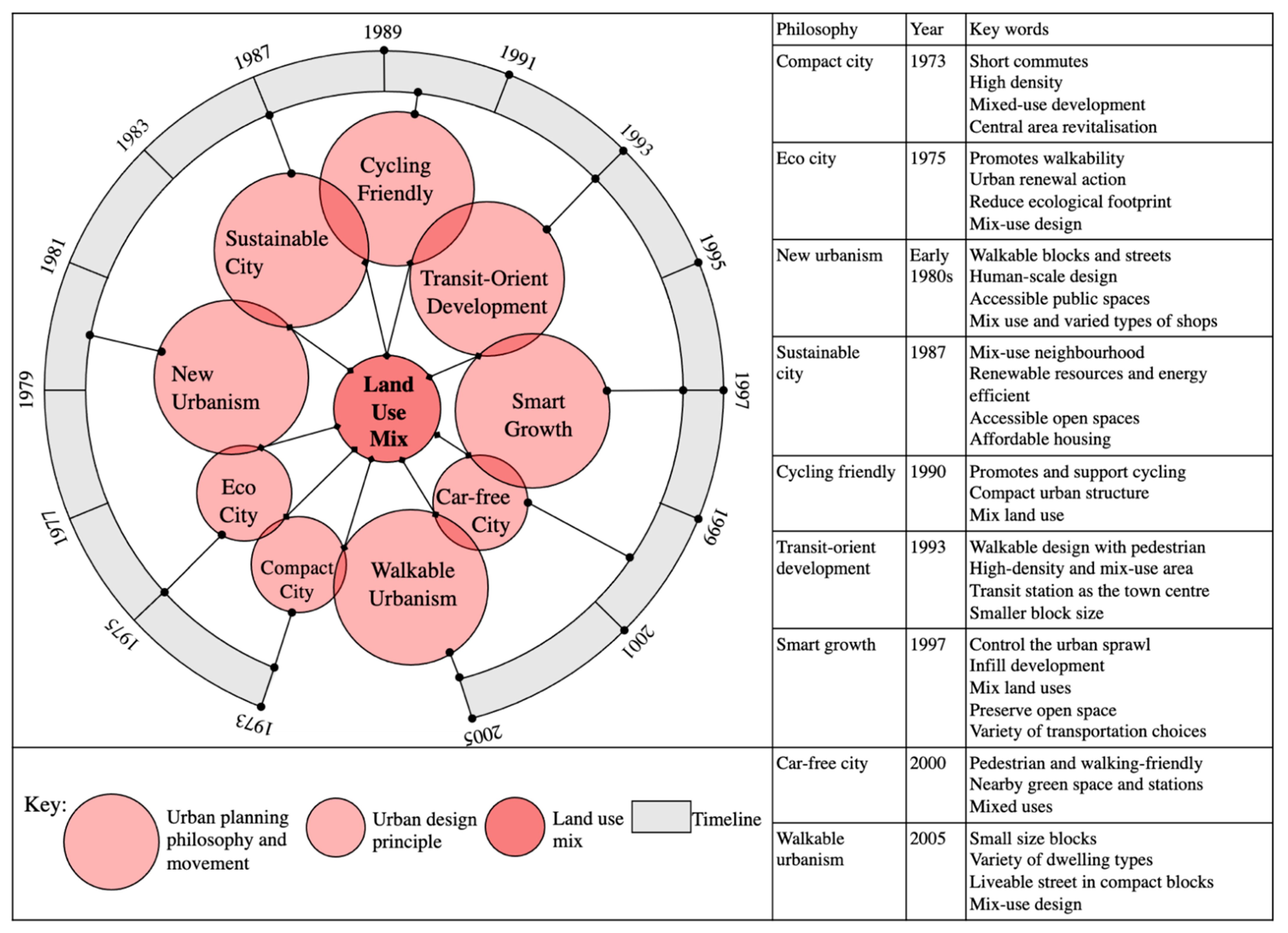
2. Literature Review

The knowledge base underpinning landscape structure and land-use mix design, initiated by Jane Jacobs with her work on “The Death and Life of Great American Cities” [2], is both broad and extensive and has been a crucial element in planning philosophies and design principles from 1973 to 2005 with a shared aim of achieving greater sustainability in city development. For example, the mix-use design is the major component in compact cities [8,9], eco-cities [10], cycling-friendly cities [11], and car-free cities [12,13]. It has been a critical component in urban planning philosophies such as new urbanism [14], sustainable development [15], transit-oriented development (TOD) [16], smart growth [17], and walkable urbanism [18] (see Figure 1).

There are several directions for the quantitation of land-use mix. One way is the quantification of land-use mix degree and exploration of the correlation between the built environment variables (e.g., urban density, distance, destination accessibility, and the transportation network structure) and personal trips in cities [19,20,21,22]. Cervero and Kockelman [19] discuss the relationship between density, travel demand, and land-use diversity in their findings in the 1990s. The evidence they present on San Francisco indicates that compact development has a substantial influence on personal business trips. Density, diversity, and design (the 3Ds) affect travel demand and mode choice [19,21]. For instance, the high level of land-use mix will promote the pedestrian mode choice of nonwork trips. Lu et al. [22] questioned the relationship between commuting mode choice and density, diversity, design, destination accessibility, distance to transit (the 5Ds) in 2018. The results established that density and diversity of land-use affect mode choice and reduce the individual mile travel (VMT) and station-based average travel distances (ATDs) [3,23].

The benefit of mixed land-use is the ability to locate multiple types of function (residential, commercial, institutional, and recreational) within a walkable or cycling-friendly distance [14]. First, land-use policies highlighted that mix-use design is an effective way to promote nonautomobile travel modes [24,25,26]. Gehrke [4] suggested that mixed land use, as a strategy, has a significant relationship with walking at the microlevel. Furthermore, other studies mentioned a positive association of active commuting, accessibility, and walkability through mixed land use [27,28,29]. In addition, the study by Heinen et al. [30] indicates that a greater level of land-use mix was associated with cycling commuting. Heinen et al. and Yang et al. [30,31] stated that mixed land use is a factor contributing to shortening travel distances and has a positive effect on cycling. Yang et al. [31] also considered the impact of terrain slope and the availability of cycling paths on cycling behaviors with respect to land-use mix. Finally, the land-use mix has also been related to neighborhood satisfaction [32,33], neighborhood crime [34], and housing price [35].

This paper has reviewed a significant cross-section of research papers and reports with respect to land-use mix [19,20,21,22,23,24,25,26,27,28,29,30,31,32,33,34,35,36,37,38,39,40,41,42,43,44,45,46,47,48,49,50,51,52,53,54,55,56,57,58]. However, while the Sankey diagram in Figure 2 illustrates the flows of land-use mix and relevant research fields, the available literature and research do not explain the applicable conditions, validity, or the quantitative process of land-use mix measures. Furthermore, neither has the diversity of land-use types been accounted for or presented by the land-use mix degree by indices. Therefore, in order to fill this research gap, our paper presents an analysis which determines the validity and applicable conditions of indices based on the definition of land-use diversity, evenness, and balance (see Figure 2).

3. Methodology

3.1. Study Design

This study aims to explore the hidden dimension of land-use mix indices. The correlation of land-use mix degree, land-use diversity, and the land-use balance is the objective of this research and was tested through a randomized control trial (RCT) using 10 virtual blocks, selected as the experimental group with a balanced mix of land uses, against a control group of 217 blocks from the City of Melbourne’s Central Business District. The benefit of the RCT is that the research decides randomly as to which urban city blocks in the trial are being tested, while the control group aims to comprise or reference the randomized group [59].

We propose a three-step screening research method to integrate the analytics processes of the comparative trial, along with a correlation analysis (see Figure 3). The RCT was used to test the efficacy of the indices being correlated.

The three-step screening process comprises the research framework of our study (see Figure 3). The first selection relies on the filtration conditions (research, applicable scale, and data precision) and discusses various aspects of the nine indices being considered. The Entropy index (ENT), Herfindahl–Hirschman index (HHI), and Dissimilarity index-II (DIS-II) comprise the second screening with respect to spatial features and land-use classification. In the third screening layer, an in-depth discussion and conclusion illustrate the inherent characteristics of the Balance index (BAL), ENT, HHI, and Dissimilarity index-I (DIS-I).

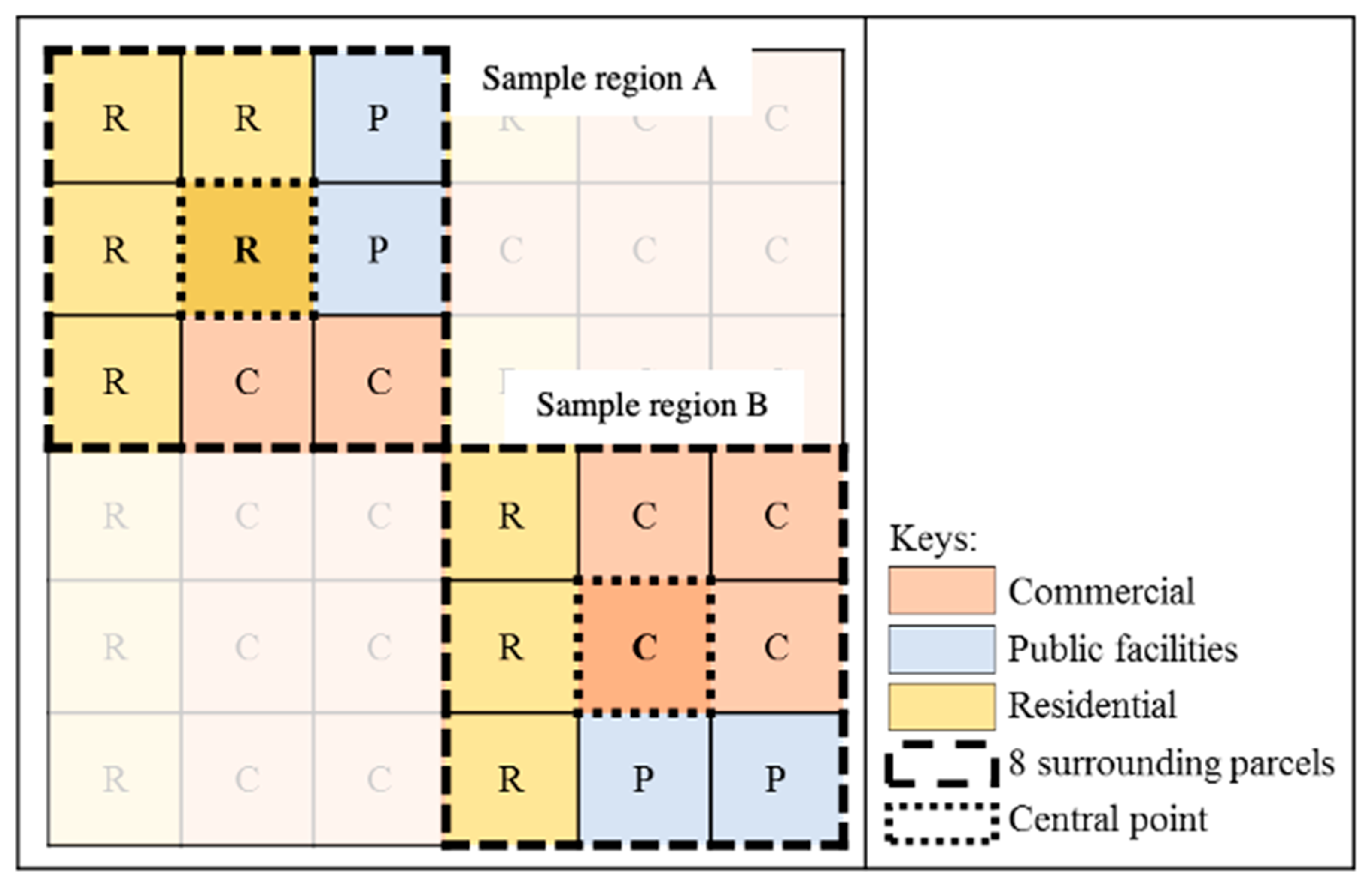
3.2. Research Method

The first screening involves nine frequently used indices. In the first step, the applicable research scale and data precision were identified based on the structure of measures. Indices were categorized into independent and complex indices. The RCT was applied to the second and third screenings. In the second and third screenings, the result of Pearson correlation’s coefficient illustrates the correlation between mix-use degree, diversity, evenness, and balance.

In the third screening, the validity variables among diversity, evenness, and balance were based on different measures. “n” is the number of land-use types of the blocks and presents the diversity directly. The balance status was calculated by the ratio of residential to nonresidential land use and accommodation to job land use. The Alatalo index is a widely used method to measure the evenness of species in previous studies and has therefore been adopted in this study [60,61]. The Alatalo evenness index is shown as follows:

$$ALT=\frac{\frac{1}{D}-1}{\exp \left(H^{\prime }\right)-1}$$

(1)

$$D=\frac{\mathrm{S}}{\sqrt{\mathrm{N}}}$$

(2)

$$H^{\prime }=-{\displaystyle \sum }_{i=1}^n{P}_i\times \ln p_i$$

(3)

ALT is the Alatalo evenness index of the given area; D is the Menhinnick evenness index; $H^{\prime }$ is Shannon–Wiener evenness index; $P_i$ is the percentage of each type of land-use in zone i; S is the number of land-use types.

Collectively, the correlation analysis was based on the IBM SPSS 26.0. The results show the correlation between mix-use degree, diversity, evenness, and balance.

3.3. Land-Use Mix Index

From the review of research papers and reports focusing on land use, most of the studies considered the ENT, DIS-I, and HHI as the effective methods to quantify the land-use mix. In this paper, we utilized the latest indices for an overall discussion of land-use mix indices. In this study, we defined nine indices into two categories. First, independent indices were used to describe those indices which only required land-use information in the calculating process. According to the review of model structure, the independent indices included: the BAL, ENT, HHI, DIS-I, and DIS-II.

Entropy index: the ENT has been used in previous studies to measure the land-use mix status. The term ENT highlights the mixture of multiple types of land use in the given area [62,63]. The equation of the ENT is shown as follows:

$$\mathrm{ENT}=-\frac{\left[{\sum }_{i=1}^k{P}^{i}ln\left(P^i\right)\right]}{ln\left(k\right)}$$

(4)

where $P^i$ is the percentage of each type of land use in zone i; k is the number of land-use types in zone i, and k ≥ 2.

Herfindahl–Hirschman Index: the term HHI has been applied to the situation of market concentration in economics and refers to land-use mixed status [64,65]. The HHI is shown as follows:

$$\mathrm{HHI}={\displaystyle \sum }_{i=1}^k{\left(100\times P^i\right)}^2$$

(5)

$P^i$ is the percentage of land use i in the given area; k is the number of land-use types in zone i.

Dissimilarity index-I: scholars believed that DIS-I is a way to measure the balance status of land-use mix in the given area [62]. DIS-I developed by Duncan [66] is shown as follows:

$$\mathrm{DIS-I}=0.5{\displaystyle \sum }_{i=1}^n\left|r_i-s_i\right|$$

(6)

where $r_i$ is the percentage of residential land use in district i; $s_i$ is the percentage of nonresidential land in district i; n is the number of districts in the area.

Dissimilarity index-II: Cervero and Kockelman [19] present a “Dissimilarity index” to discuss the land-use diversity around the central parcel in the San Francisco study and classify land-use type as residential, commercial, office, industrial, institutional, park, and recreation (Figure 4). In this study, Dissimilarity index by Cervero and Kockelman [19] was labelled as DIS-II. DIS-II is shown as follows:

$$\mathrm{DIS-II}=\frac{\left[{\sum }_i^K{\sum }_l^8\left(\frac{X_l}{8}\right)\right]}{K}$$

(7)

where K is the total area of surrounding parcels around the central point; $X_l$ is the number of parcels with different land-use type/types with the central parcel; l is the type of land use in the central area.

Complex indices require more information in the quantification process (spatial location, adjust factor, and number of trips in blocks) as the component structure of complex indices is more intricate than independent indices. For example, some measures were weighted with an economic factor to the land-use measures such as the Clustering index (CLTS) and Gini index (GINI).

Clustering index: the model structure of the CLTS not only involves the areas of residential land and nonresidential land but also considers the spatial distances between the centroids of pairs of districts [62,67]:

$$\mathrm{CLST}=\frac{{\sum }_{i=1}^n{S}_i{\sum }_{i^{*}}^n{Y}_i\times e^{-d_{i{i}^{*}}}-\frac{Y}{n^2}{\sum }_{i=1}^n{\sum }_{i^{*}}^n{e}^{-d_{i{i}^{*}}}}{{\sum }_{i=1}^n{S}_i{\sum }_{i^{*}=1}^n{Z}_i\times e^{-d_{i{i}^{*}}}-\frac{Y}{n^2}{\sum }_{i=1}^n{\sum }_{i^{*}}^n{e}^{-d_{i{i}^{*}}}}$$

(8)

Y is the area of nonresidential land; $S_i$ is the percentage of nonresidential land in district i; $Z_i$ is the area of district i; $Y_i$ is the area of nonresidential land of district i; $d_{i{i}^{*}}$ is the distance between distance i and the center of district $i^{*}$; n is the total area of the district.

Gini index: the GINI, developed by Corrado Gini [68], applies measures such as economic inequality and urban studies [68]:

$$\mathrm{GINI}=\left|1-{\displaystyle \sum }_{i=1}^n\left(\sigma r_{i+1}+\sigma r_i\right)\left(\sigma s_{i+1}-\sigma s_i\right)\right|$$

(9)

$r_i$ is the proportion of residential land in district i; $s_i$ is the proportion of nonresidential land in district i; σ is the adjust parameter.

The activity-related complementarity (ARC) model was used to describe the land-use mixed pattern [20]. The ARC model integrates the proportion of multiple types of land use and the number of trips generated by a single type of land use into one model:

$$\mathrm{ARC}=1-{\displaystyle \sum }_{i=1}^n\left(P_i\times \frac{\left|P_i-F_i\right|}{1-F_i}\right)$$

(10)

n is the number of land-use types; $P_i$ is the percentage of land-use type i in a given area; $F_i$ is an activity adjust factor and reflects number of trips generated by a single type of land use.

Mix degree index: the complex index takes spatial features into account in the quantitative process. For example, Tian et al. proposed a mix degree index (MDI) to measure the mixture of residential and industrial lands in the peri-urban areas in China [1]. Tian et al. [1] also categorized the land-use types as residential. Each type of land use was assigned a value from 0 to 3, and the spatial and land-use types influenced the value of MDI (Figure 5). The MDI is expressed as follows:

$$\mathrm{MDI}={\displaystyle \sum }_{i=1}^n\frac{n_i}{\left(n\times 25\right)}$$

(11)

where n is the number of grids cover by residential landscape in a given area; $n_i$ is the mixed degree of a residential patch i in the given area; 25 is the maximum assigned value of mixed degree of sample region (see Figure 5).

3.4. Data Collection

Melbourne is the capital city of the state of Victoria, Australia. The road network and the street blocks in the Central Business District are formed according to a Hoddle street grid (see Figure 6). Sidewalk Labs [69] points out that the benefits of a regular street grid include: (i) the ease of of building or rebuilding; (ii) ease of navigation, especially for new people coming to visit or live in the city; (iii) traffic being able to be rerouted during street closures or peak traffic conditions.

Furthermore, the grid-like streets divide the city into similarly shaped blocks of similar sizes, facilitating same-scale quantifiable land-use information collected for each block from the Census of Land Use and Employment (CLUE).

In this study, land-use information of 217 blocks in the CLUE only covers the percentages of each type of land use. The spatial locations of different land-use types were not given in the CLUE. We designed 10 virtual block groups (see Figure 7), all with balanced land-use mixes in order to isolate balance and evenness as constants. In addition, the random locations of the different land-use tests and the diversity of the type of land-uses were independent variables. The designs of 10 virtual blocks are shown in Figure 7. Blocks EG-01 to EG-10 have a balanced proportion of different types of land uses. The independent variables of block EG-01 to EG-10 are the number of land-use types and the spatial locations of each type of land use. For example, the subgroup (named EG-04(a)) had the same proportion of land-use types, but all of them had different spatial features. The results of the analysis of 10 virtual blocks identified the influence level of spatial features in land-use mix quantitation and provided further exploration of data precision.

The review of previous studies establishes several standards of land-use classification. For example, for the land-use mix pattern by the ENT, Gan et al. [23] identified seven categories of land-use information within the ENT including: administrative, business, commercial, green space, industrial, residential and other. Shashank and Schuurman [70] classified land-use data as commercial, residential, and office due to the moderate compatibility of the dataset. For the six-category index, institutional (or health care), entertainment, and physical activities were extracted from the land-use classification. However, institutional health care was excluded from the five-category HHI index due to the lack of available data.

The classification standards of land use depended on the research objectives, study background, and the source of data. We classified the categorization of land based on the Australian and New Zealand Standard Industrial Classification (ANZSIC) [71]. Beyond this classification, we detailed and summarized subtype 1 and subtype 2 and applied the respective data in the land-use balance analysis (

Table 1. The classification of land-use types by Australian and New Zealand Standard Industrial Classification (ANZSIC).

Main Types	Subtype 1	Subtype 2	Details
Residential	Residential	Residential	Accommodation
Nonresidential	Jobs	Administration and public service	Admin and support services, education and training, health care and social assistance, public administration and safety.
		Commercial and business facilities	Business services, finance and insurance, information media and telecommunications; manufacturing, food and beverage services, real estate services, rental and hiring services, retail trade, wholesale trade.
	Recreation	Leisure and recreation facilities	Arts and recreation services.
	Others	Others	Agriculture and mining, construction, electricity, gas, water and waste services, other services, transport, postal and storage, others.

). Moreover, the land-use details of 217 blocks are based on the CLUE database [7]. The data cover the period 2002 to 2018, and we collected the data in 2018. A total of 217 blocks located in the suburbs of Kensington, North Melbourne, Carlton, Melbourne, Southbank, and Docklands served as the primary source of the control group to explore the potential characteristics of land-use mix indices.

4. Results and Discussion

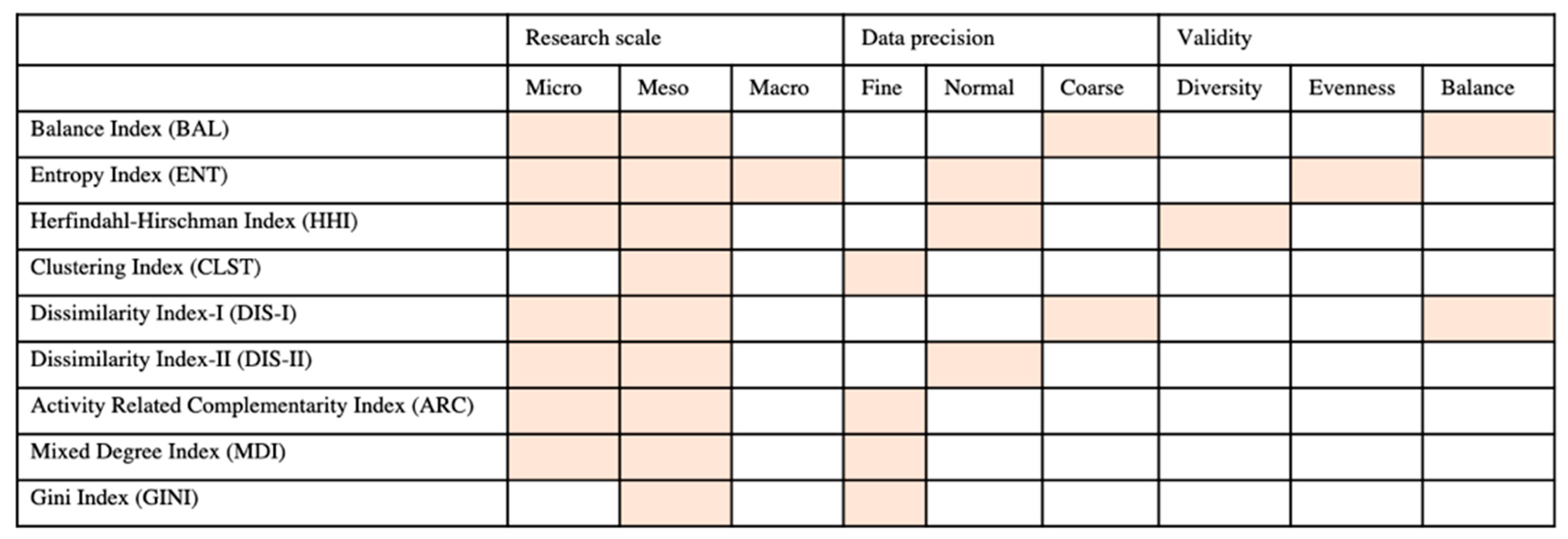
4.1. Finding of First Screening

Data precision is an aspect to discuss the hidden features of land-use mix indices. In this research, we define the data precision levels by the requirements of data collection. Most of the land-use mix measures required land-use details with specific areas or percentages; however, we define the data precision in this level of data collection as negligible. Furthermore, some land-use mix indices and the number of land-use types in the measurement have been defined with an average level of data precision based on the dataset with areas (or percentages) and the number of land-use types. The review of previous studies also highlighted the spatial location and the demographic information within the calculation of land-use mix degree—we define the precision level of these indices as a finite level.

The conclusion of the review emphasizes the research scales and data precision of indices (

Table 2. The applicable research scale and data precision conditions of indices.

	Research Scale			Data Precision
	Micro (Block)	Meso (District)	Macro (City)	Fine	Normal	Coarse
Balance Index (BAL)	+	+				+
Entropy Index (ENT)	+	+	+		+
Herfindahl-Hirschman Index (HHI)	+	+			+
Clustering Index (CLST)		+		+
Dissimilarity Index-I (DIS-I)	+	+				+
Dissimilarity Index-II (DIS-II)	+	+			+
Activity-Related Complementarity (ARC) Index	+	+		+
Mixed Degree Index (MDI)	+	+		+
Gini Index (GINI)		+		+

“+”. Applicable to the current condition.

). This study focused on the exploration of the potential characteristics of land-use mix indices at the block and neighborhood levels. The further discussion of the validity of indices land-use information of the control group only covers the areas and percentages of each type of land use. Under this situation, the second and third screenings only discuss the BAL, ENT, HHI, DIS-I, and DIS-II, due to the limitation of data collection.

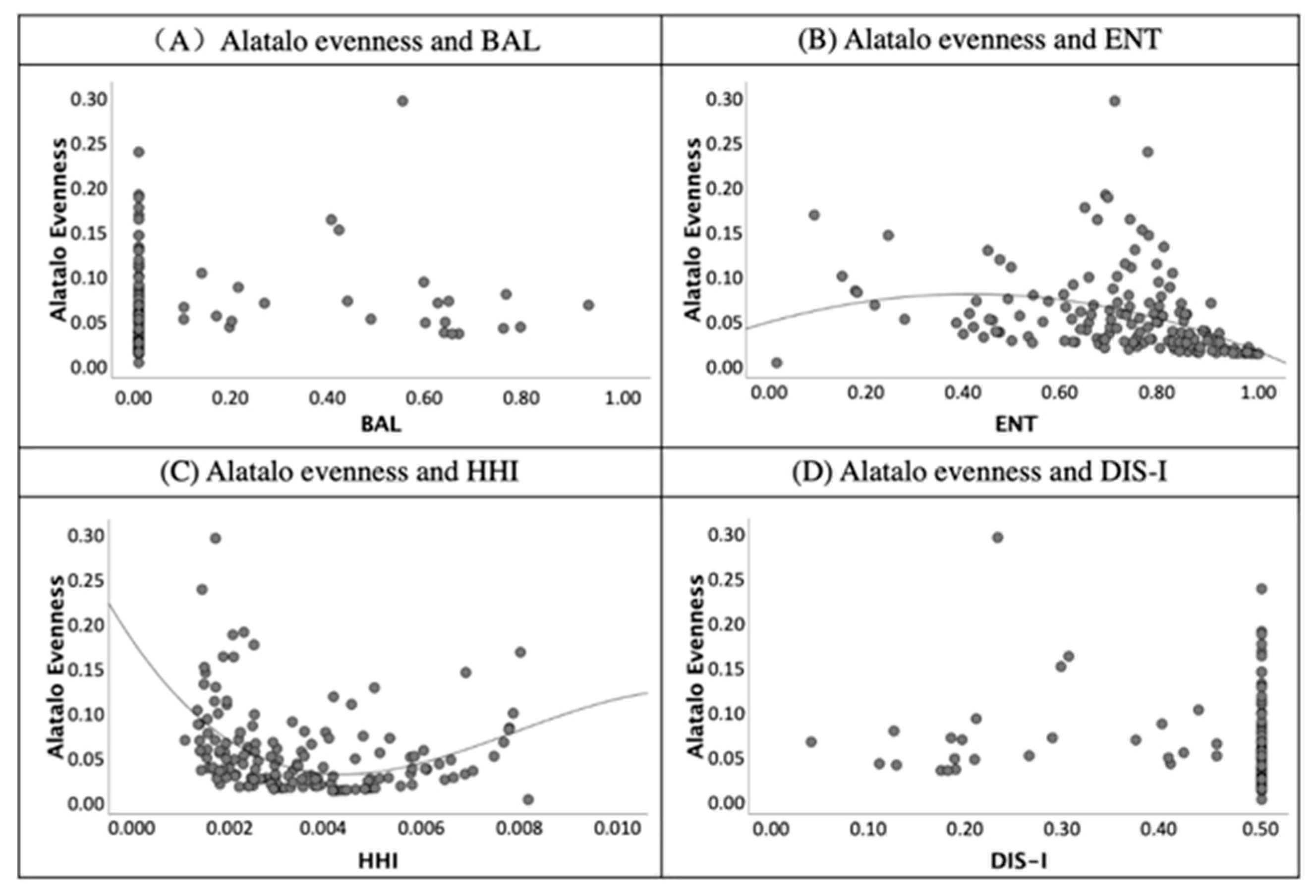
4.2. Finding of Second Screening

According to the findings of the preliminary selection, we used five measures in the second and third screenings. The values represent various features of land-use mix indices.

In

Table 3. The land-use details of virtual blocks, land-use diversity (n), and the land-use mix degree.

	Land Use Details (%)											Land-Use Mix Degree
	Land use-1	Land use-2	Land use-3	Land use-4	Land use-5	Land use-6	Land use-7	Land use-8	Land use-9	Land use-10	n	ENT	HHI	DIS-II (a)	DIS-II (b)	DIS-II (c)
EG-01	100.0	0	0	0	0	0	0	0	0	0	1	N/A	10,000.0	0.0	N/A	N/A
EG-02	50.0	50.0	0	0	0	0	0	0	0	0	2	1.0	5000.0	0.5	N/A	N/A
EG-03	33.3	33.3	33.3	0	0	0	0	0	0	0	3	1.0	3333.3	0.8	N/A	N/A
EG-04	25.0	25.0	25.0	25.0	0	0	0	0	0	0	4	1.0	2500.0	0.0	0.6	N/A
EG-05	20.0	20.0	20.0	20.0	20.0	0	0	0	0	0	5	1.0	2000.0	0.0	0.8	N/A
EG-06	16.7	16.7	16.7	16.7	16.7	16.7	0	0	0	0	6	1.0	1666.7	0.0	0.9	0.8
EG-07	14.2	14.2	14.2	14.2	14.2	14.2	14.2	0	0	0	7	1.0	1411.5	0.0	0.8	N/A
EG-08	12.5	12.5	12.5	12.5	12.5	12.5	12.5	12.5	0	0	8	1.0	1250.0	0.0	0.9	0.9
EG-09	11.1	11.1	11.1	11.1	11.1	11.1	11.1	11.1	11.1	0	9	1.0	1108.9	0.0	1.0	N/A
EG-10	10.0	10.0	10.0	10.0	10.0	10.0	10.0	10.0	10.0	10.0	10	1.0	1000.0	0.0	1.0	0.0

, “n” presents the diversity of land-use types; values in the ENT column are the land-use mix degree were calculated by the ENT; values in the HHI column present the mixed degree calculated by the Herfindahl–Hirschman index; values in the DIS-II (a) column indicate the land-use mixed degree calculated by Dissimilarity index-II with the land-use status (a). Values in DIS-II (b) column indicate the land-use mixed degree calculated by Dissimilarity index-II with the land-use mixed status (b). Values in DIS-II (c) column indicate the land-use mixed degree calculated by Dissimilarity index-II with the land-use mixed status (c).

The values of EG-01 to EG-10 of the ENT highlight that the ENT is only workable for the parcel with more than two types of land use. As the number of land-use types increases, the value of the ENT is the same (ENT = 1) in the 10 experimental groups. Thus, the values of the ENT do not reflect land-use diversity.

Furthermore, EG-01 to EG-10 showed a negative correlation between the number of land-use types and mixed degree. The results of the experimental group may indicate that the values of the HHI reflect land-use diversity.

Finally, we simulated several spatial distributions based on the proportion of the different types of land use. The results are categorized as DIS-II (a), DIS-II (b), and DIS-II (c). Furthermore, the values identified the features of DIS-II, indicating that spatial distribution affects the values of DIS-II. The feasibility condition of land-use pattern and land-use distribution in the city is more complicated than the 10 experimental groups. In order to disclose the hidden characteristics, we applied land-use details of 217 blocks in the city of Melbourne in the third screening.

4.3. Finding of Third Screening

The results of the secondary screening highlighted that the HHI is related to the diversity of land-use type (Table 3). However, the validities of the BAL, ENT and DIS-II were not shown in Table 3. The scatter diagrams of the validity indices are presented in Figure 8, Figure 9, Figure 10 and Figure 11. Examining Figure 8, only the HHI was related to the diversity value. The BAL and DIS-I did not correlate with the diversity value (n)—BAL is 0.00 and DIS-I is 0.50—and the diversity value (n) presented an inverse relationship when comparing graphs (A) and (D). According to the finding in graph (C) in Figure 8, the HHI is the index related to the diversity of land-use types.

Second, both the BAL and DIS-I are related to the ratio of residential and non-residential (RRN) according to the linear relationship in Figure 9. The BAL and DIS-I show mirror-image symmetry. According to this, the validities of the BAL and DIS-I are the same. Unlike the BAL, DIS-I was negatively correlated to RRN. Graphs (A) and (D) in Figure 9 prove that both the BAL and DIS-I correlated with residential land and nonresidential land balance statuses.

In Figure 10, a similar correlation was shown between the BAL to RAJ (balance ratio of accommodation and job). Moreover, a positive correlation is presented in the graph (A). In contrast, the values of RAJ and DIS-I had a negative relationship according to graph (D) of Figure 10. Additionally, the correlation between the BAL and RAJ illustrates that the BAL’s values reflect the balance between two different land uses.

For the test results of evenness’s validity, the Alatalo evenness index was used to present the evenness of land-use mix of blocks. In Figure 11, both the ENT and HHI were related to Alatalo evenness. Graph (B) and graph (C) present a correlation of indices. Nevertheless, the values of the BAL and DIS are not related to the evenness indices (see Figure 11).

For further comparison of the correlation between the index’s validity of diversity, evenness, and balance, the correlation coefficients are shown in

Table 4. The correlation coefficients of validity indices and land-use mix indices.

		Diversity (n)	Balance (RRN)	Balance (RAJ)	Alatalo Evenness
BAL	Pearson Correlation	0.28 **	0.69 **	0.70 **	0.17 *
	Sig. (2-tailed)	0.00	0.00	0.00	0.03
ENT	Pearson Correlation	0.13	−0.13	−0.13	−0.31 **
	Sig. (2-tailed)	0.09	0.11	0.11	0.00
HHI	Pearson Correlation	−0.81 **	−0.10	−0.09	−0.20 *
	Sig. (2-tailed)	0.00	0.16	0.21	0.01
DIS-I	Pearson Correlation	−0.28 **	−0.69 **	−0.70 **	−0.17 *
	Sig. (2-tailed)	0.00	0.00	0.00	0.03

Total sample is 217 and valid sample is 161. **. Correlation is significant at the 0.01 level (2-tailed). *. Correlation is significant at the 0.05 level (2-tailed).

. According to Pearson’s correlation coefficient, a discussion of the correlation between the validity indices and land-use mix indices is presented below.

First, the BAL correlates to the validity indices of RRN and RAJ due to the coefficients being 0.69 and 0.70 and significant at the 0.01 level. Most of the studies assumed that the value of ENT reflects the diversity of land-use types. However, only the index of Alatalo evenness correlates to the ENT significantly at the 0.01 level in Table 4. This finding supports that the ENT is the measure to quantify the evenness of land-use rather than the diversity. According to the correlation coefficients of validity indices and the HHI, a positive correlation was shown between diversity (n) and the HHI. Moreover, the negative correlation illustrates the correlation coefficients of RRN to DIS-I (−0.69) and RAJ to DIS-I (−0.70).

Overall, the validity and features of land-use indices were concluded based on the comparison of the experimental group and the control group. In the results of second screening, only the HHI is related to the diversity of land-use type (n), and the ENT, DIS-I, and DIS-II were not related to the land-use diversity according to the analysis of 10 virtual blocks. Furthermore, the calculation process of DIS-I requires a precise classification of land-use types and not land-use mix degree. DIS-II was influenced by the spatial location of lands with different land-use characteristics. Land-use mix indices of the ENT is applicable for the given area with over two types of land use. The findings of the third screening prove the findings of the second screening—i.e., that the HHI is correlated to the land-use diversity validity index. Moreover, the BAL is applicable for the land-use balance studies because of a high level of the correlation coefficient between the BAL and balance ratios of RRN and RAJ. Additionally, the ENT correlates to the validity index of Alatalo evenness and is applicable for land-use evenness studies. The findings of the three-step screening analysis will inform application and decision-making in sustainable city development.

5. Conclusions and General Recommendations

5.1. Research Conclusions

In this study, we conducted and updated the review of land-use mix research from both theoretical and quantitative aspects. The review of previous literature was based largely on empirical studies. According to the conclusion of the literature review, few studies have explored the validity of land-use mixed indices. The three-step screening method for the research was based on the knowledge gap in the analyses of data precision and validity of land-use mix measures, involving nine indices that have remained largely unexplored.

The primary selection relies on the first screening of the model structure of eight indices which highlight the applicable scale and data precision of the indices. All of the indices can be applied to quantitation of land-use mix of blocks or districts. However, due to the limitation of the dataset and lack of information of the spatial condition of land use, the indices of the CLST, ARC, MDI, and GINI were not applied to the second and third screenings.

After the primary screening, five indices were selected and applied to the second screening. In total, 10 virtual blocks with balance statuses formed the experimental group in the second screening, which aimed to isolate the influence of the independent variables (diversity and spatial contribution) and eliminate the irrelevant effects variables (evenness, balance, and categorization of land use). The result highlights several findings. First, the ENT is applicable for the block with more than two types of land use, due to the structure of the models. Second, a correlation was found between land-use diversity (n) and the HHI. With the increase in the type of land use, the value of HHI decreased. The values of the BAL and DIS-I were not available due to the land-use categorization being eliminated as an irrelevant variable. In addition, the spatial contribution was proved to be a relevant variable that potentially affects the value of DIS-II. In the third screening, DIS-II was eliminated because of the lack of spatial information for the dataset.

The third screening identified the correlation between land-use mix indices and validity. Several studies mentioned the ENT as a means to present the diversity of land-use mixed statuses. However, the findings of the third screening against the correlation of land-use diversity and the value of the ENT highlighted that the ENT only relates to the evenness of land use. DIS-I and the BAL positively related to both a balanced status of residential to nonresidential land and accommodation to job. According to the correlation coefficients, the BAL was positively related to the balance of land use, and DIS-I was negatively related to the balance status. The HHI was the most suitable measure to quantify the diversity of land use among the blocks due to a direct and negative correlation revealed in both the second and third screenings.

5.2. General Recommendations

Based on the application conditions of the nine land-use indices considered in the paper (see Figure 12), the following presents the following general recommendations.

First, the applicable condition of the Gini index is a localized one and is only suitable for research at the medium scale with an adequate dataset.

Second, while the BAL and DIS-I indicated lower thresholds based on a wide range of research, scale, and coarse data precision, they were nonetheless suitable for the study, which aimed to understand the balance status of land use.

Third, the discussion of the land-use diversity in the micro to medium scales should be based on the HHI rather than the ENT when undertaking further research.

Further research could attempt to compare across contexts in order to test variability and multiscale applications. Index comparisons could be extended to include additional sustainability, ecological service systems resources, environmental impacts, and socio-cultural and qualitative interfacing, as these are coeffectual and interoperational.

While the application of these indices is currently highly specialized, establishing an interface which enables them to be an effective tool to assist more holistic planning processes and to inform best practice for design professionals would be a significant step forward in achieving greater sustainability in future city development.

References

1. Tian, L.; Liang, Y.; Zhang, B. Measuring residential and industrial land use mix in the peri-urban areas of China. Land Use Policy 2017, 69, 427–438. [Google Scholar] [CrossRef]
2. Jacobs, J. The Death and Life of Great American Cities; Random House: New York, NY, USA, 1961. [Google Scholar]
3. Ewing, R.; Cervero, R. Travel and the Built Environment. J. Am. Plan. Assoc. 2010, 76, 265–294. [Google Scholar] [CrossRef]
4. Gehrke, S.; Clifton, K.J. Toward a spatial-temporal measure of land-use mix. J. Transp. Land Use 2015. [Google Scholar] [CrossRef] [Green Version]
5. Mavoa, S.; Eagleson, S.; Badland, H.; Gunn, L.D.; Boulangé, C.; Stewart, J.; Giles-Corti, B. Identifying appropriate land-use mix measures for use in a national walkability index. J. Transp. Land Use 2018, 11. [Google Scholar] [CrossRef]
6. Reliability vs Validity in Research|Differences, Types and Examples. Available online: https://www.scribbr.com/methodology/reliability-vs-validity/ (accessed on 30 October 2020).
7. CLUE Small Area and Block Maps—City of Melbourne. Available online: https://data.melbourne.vic.gov.au/Business/Floor-space-by-block-by-ANZSIC/a9sc-9jxz (accessed on 25 September 2020).
8. Dantzig, G.; Saaty, T. Compact City: A Plan for a Liveable Urban Environment; W.H. Freeman and Comp.: San Francisco, CA, USA, 1973. [Google Scholar]
9. Vallance, S.; Perkins, H.; Dixon, J. Compact Cities: Everyday Life, Governance and the Built Environment; School of Architecture and Planning, University of Auckland: Auckland, New Zeeland, 2009. [Google Scholar]
10. Roseland, M. Dimensions of the eco-city. Cities 1997, 14, 197–202. [Google Scholar] [CrossRef]
11. Wheeler, S.; Beatley, T. Sustainable Urban Development Reader, 2nd ed.; Routledge: London, UK, 2014. [Google Scholar]
12. Crawford, J. Carfree Cities; International Books: Utrecht, The Netherlands, 2000. [Google Scholar]
13. Jiao, J. Analysis and Research on Car-Free City Parking System Layout. Master’s Thesis, Shandong Jianzhu University, Shandong, China, 2018. [Google Scholar]
14. Land Use Impacts on Transport: How Land Use Factors Affect Travel Behaviour; Victoria Transport Policy Insititute, 2019; Available online: https://www.vtpi.org/landtravel.pdf (accessed on 6 October 2020).
15. Report of the World Commission on Environment and Development: Our Common Future; Oxford University Press: Oxford, UK, 1987; Available online: http://www.un-documents.net/wced-ocf.htm (accessed on 6 October 2020).
16. Calthorpe, P.; Poticha, S. The Next American Metropolis; Princeton Architectural Press: New York, NY, USA, 1993. [Google Scholar]
17. APA Policy Guide on Smart Growth. Available online: https://www.planning.org/policy/guides/adopted/smartgrowth.htm (accessed on 29 October 2020).
18. Southworth, M. Designing the Walkable City. J. Urban Plan. Dev. 2005, 131, 246–257. [Google Scholar] [CrossRef]
19. Cervero, R.; Kockelman, K. Travel demand and the 3Ds: Density, diversity, and design. Transp. Res. Part D Transp. Environ. 1997, 2, 199–219. [Google Scholar] [CrossRef]
20. Gehrke, S. Land Use Mix and Pedestrian Travel Behavior: Advancements in Conceptualization and Measurement. Ph.D. Thesis, Portland State University, Portland, OR, USA, 2017. Available online: https://www.semanticscholar.org/paper/Land-Use-Mix-and-Pedestrian-Travel-Behavior%3A-in-and-Gehrke/9745b4556015a815495bf0cf3c198aade6a2a464 (accessed on 6 October 2020).
21. Lee, C.; Moudon, A.V. The 3Ds+R: Quantifying land use and urban form correlates of walking. Transp. Res. Part D Transp. Environ. 2006, 11, 204–215. [Google Scholar] [CrossRef]
22. Lu, Y.; Sun, G.; Sarkar, C.; Gou, Z.; Xiao, Y. Commuting Mode Choice in a High-Density City: Do Land-Use Density and Diversity Matter in Hong Kong? Int. J. Environ. Res. Public Health 2018, 15, 920. [Google Scholar] [CrossRef] [PubMed] [Green Version]
23. Gan, Z.; Feng, T.; Wu, Y.; Yang, M.; Timmermans, H. Station-Based Average Travel Distance and Its Relationship with Urban form and Land Use: An Analysis of Smart Card Data in Nanjing City, China. Transp. Policy 2019, 79, 137–154. [Google Scholar] [CrossRef]
24. Christian, H.; Bull, F.; Middleton, N.; Knuiman, M.; Divitini, M.; Hooper, P.; Amarasinghe, A.; Giles-Corti, B. How Important Is the Land Use Mix Measure in Understanding Walking Behaviour? Results from the RESIDE Study. Int. J. Behav. Nutr. Phys. Act. 2011, 8, 55. [Google Scholar] [CrossRef] [Green Version]
25. McConville, M.E.; Rodriguez, D.A.; Clifton, K.; Cho, G.; Fleischhacker, S. Disaggregate Land Uses and Walking. Am. J. Prev. Med. 2011, 40, 25–32. [Google Scholar] [CrossRef]
26. Zhang, M.; Zhao, P. The impact of land-use mix on residents’ travel energy consumption: New evidence from Beijing. Transp. Res. Part D Transp. Environ. 2017, 57, 224–236. [Google Scholar] [CrossRef]
27. Diao, M. Selectivity, spatial autocorrelation and the valuation of transit accessibility. Urban Stud. 2015, 52, 159–177. [Google Scholar] [CrossRef] [Green Version]
28. MacKenbach, J.D.; Randal, E.; Zhao, P.; Chapman, R. The Influence of Urban Land-Use and Public Transport Facilities on Active Commuting in Wellington, New Zealand: Active Transport Forecasting Using the WILUTE Model. Sustainability 2016, 8, 242. [Google Scholar] [CrossRef] [Green Version]
29. Song, S.; Diao, M.; Feng, C.-C. Individual transport emissions and the built environment: A structural equation modelling approach. Transp. Res. Part A Policy Pr. 2016, 92, 206–219. [Google Scholar] [CrossRef]
30. Heinen, E.; Van Wee, B.; Maat, K. Commuting by Bicycle: An Overview of the Literature. Transp. Rev. 2010, 30, 59–96. [Google Scholar] [CrossRef]
31. Yang, Y.; Wu, X.; Zhou, P.; Gou, Z.; Lu, Y. Towards a Cycling-Friendly City: An Updated Review of the Associations between Built Environment and Cycling Behaviors (2007–2017). J. Transp. Health 2019, 14, 100613. [Google Scholar] [CrossRef]
32. Kweon, B.; Ellis, C.; Leiva, P.; Rogers, G. Landscape Components, Land Use, and Neighborhood Satisfaction. Environ. Plan. B Plan. Des. 2010, 37, 500–517. [Google Scholar] [CrossRef]
33. Mouratidis, K. Is Compact City Livable? The Impact of Compact Versus Sprawled Neighbourhoods on Neighbourhood Satisfaction. Urban Stud. 2017, 55, 2408–2430. [Google Scholar] [CrossRef]
34. Wo, J.C. Mixed land use and neighborhood crime. Soc. Sci. Res. 2019, 78, 170–186. [Google Scholar] [CrossRef] [PubMed]
35. Kim, D.; Jin, J. The Effect of Land Use on Housing Price and Rent: Empirical Evidence of Job Accessibility and Mixed Land Use. Sustainability 2019, 11, 938. [Google Scholar] [CrossRef] [Green Version]
36. Badoe, D.; Miller, E. Transportation–Land-Use Interaction: Empirical Findings in North America, and Their Implications for Modeling. Transp. Res. Part D Transp. Environ. 2000, 5, 235–263. [Google Scholar] [CrossRef]
37. Baranzini, A.; Schaerer, C. A sight for sore eyes: Assessing the value of view and land use in the housing market. J. Hous. Econ. 2011, 20, 191–199. [Google Scholar] [CrossRef] [Green Version]
38. Cervero, R. City CarShare: First-Year Travel Demand Impacts. Transp. Res. Rec. J. Transp. Res. Board 2003, 1839, 159–166. [Google Scholar] [CrossRef]
39. De Groot, R. Function-Analysis and Valuation as a Tool to Assess Land Use Conflicts in Planning for Sustainable, Multi-Functional Landscapes. Landsc. Urban Plan. 2006, 75, 175–186. [Google Scholar] [CrossRef]
40. Ewing, R.; Greenwald, M.; Zhang, M.; Walters, J.; Feldman, M.; Cervero, R.; Frank, L.; Thomas, J. Traffic Generated by Mixed-Use Developments—Six-Region Study Using Consistent Built Environmental Measures. J. Urban Plan. Dev. 2011, 137, 533–555. [Google Scholar] [CrossRef]
41. Frank, L.D. Land Use and Transportation Interaction. J. Plan. Educ. Res. 2000, 20, 6–22. [Google Scholar] [CrossRef]
42. Frank, L.; Pivo, G. The Impacts of Mixed Use and Density on the Utilization of Three Modes of Travel: The Single-Occupant Vehicle, Transit, and Walking. Transp. Res. Rec. 1994, 1466, 44–52. [Google Scholar]
43. Hu, T.; Yang, J.; Li, X.; Gong, P. Mapping Urban Land Use by Using Landsat Images and Open Social Data. Remote Sens. 2016, 8, 151. [Google Scholar] [CrossRef]
44. Kim, J.; Larsen, K. Can New Urbanism Infill Development Contribute to Social Sustainability? The Case of Orlando, Florida. Urban Stud. 2016, 54, 3843–3862. [Google Scholar] [CrossRef]
45. Kleemann, J.; Baysal, G.; Bulley, H.N.; Fürst, C. Assessing driving forces of land use and land cover change by a mixed-method approach in north-eastern Ghana, West Africa. J. Environ. Manag. 2017, 196, 411–442. [Google Scholar] [CrossRef]
46. Lang, W.; Long, Y.; Chen, T. Rediscovering Chinese cities through the lens of land-use patterns. Land Use Policy 2018, 79, 362–374. [Google Scholar] [CrossRef]
47. Lu, J.; Guldmann, J. Landscape Ecology, Land-Use Structure, and Population Density: Case Study of the Columbus Metropolitan Area. Landsc. Urban Plan. 2012, 105, 74–85. [Google Scholar] [CrossRef]
48. Ma, S.; Zhang, Y.; Yu, Z. Optimization and Application of Integrated Land Use and Transportation Model in Small- and Medium-Sized Cities in China. Sustainability 2019, 11, 2555. [Google Scholar] [CrossRef] [Green Version]
49. Manaugh, K.; Kreider, T. What is mixed use? Presenting an interaction method for measuring land use mix. J. Transp. Land Use 2013, 6, 63–72. [Google Scholar] [CrossRef]
50. Mualam, N.Y.; Salinger, E.; Max, D. Increasing the urban mix through vertical allocations: Public floorspace in mixed use development. Cities 2019, 87, 131–141. [Google Scholar] [CrossRef]
51. Ratner, K.; Goetz, A. The Reshaping of Land Use and Urban Form in Denver through Transit-Oriented Development. Cities 2013, 30, 31–46. [Google Scholar] [CrossRef]
52. Soteropoulos, A.; Berger, M.; Ciari, F. Impacts of automated vehicles on travel behaviour and land use: An international review of modelling studies. Transp. Rev. 2019, 39, 29–49. [Google Scholar] [CrossRef]
53. Sung, H.; Oh, J.-T. Transit-oriented development in a high-density city: Identifying its association with transit ridership in Seoul, Korea. Cities 2011, 28, 70–82. [Google Scholar] [CrossRef]
54. Turner, B. Sustainability and forest transitions in the southern Yucatán: The land architecture approach. Land Use Policy 2010, 27, 170–179. [Google Scholar] [CrossRef]
55. Van Acker, V.; Witlox, F. Commuting trips within tours: How is commuting related to land use? Transportation 2011, 38, 465–486. [Google Scholar] [CrossRef]
56. Wei, Y.; Xiao, W.; Wen, M.; Wei, R. Walkability, Land Use and Physical Activity. Sustainability 2016, 8, 65. [Google Scholar] [CrossRef] [Green Version]
57. Yigitcanlar, T.; Dur, F. Developing a Sustainability Assessment Model: The Sustainable Infrastructure, Land-Use, Environment and Transport Model. Sustainability 2010, 2, 321–340. [Google Scholar] [CrossRef] [Green Version]
58. Zhu, Y.; Diao, M.; Ferreira, J.; Zegras, C. An integrated microsimulation approach to land-use and mobility modeling. J. Transp. Land Use 2018, 11, 633–659. [Google Scholar] [CrossRef]
59. MacGill, M. Randomized Controlled Trials: Overview, Benefits, and Limitations. Available online: https://www.medicalnewstoday.com/articles/280574 (accessed on 30 October 2020).
60. Alatalo, R.V. Problems in the Measurement of Evenness in Ecology. Oikos 1981, 37, 199. [Google Scholar] [CrossRef]
61. Wang, L.; Guo, B.; Huang, H.; Li, S.; Zhang, C.; Zhang, B.; Zhang, J. Larx Principis-Rupprechtii Species Diversity of North Ditch Forest Farm of Hebei. Heilongjiang Agric. Sci. 2018, 4, 88–91. [Google Scholar]
62. Song, Y.; Merlin, L.; Rodriguez, D. Comparing measures of urban land use mix. Comput. Environ. Urban Syst. 2013, 42, 1–13. [Google Scholar] [CrossRef]
63. Song, Y.; Knaap, G.-J. Measuring the effects of mixed land uses on housing values. Reg. Sci. Urban Econ. 2004, 34, 663–680. [Google Scholar] [CrossRef]
64. Hirschman, A. National Power and the Structure of Foreign Trade; University of California Press: Berkeley, CA, USA, 1945. [Google Scholar]
65. Hirschman, A. The Paternity of an Index. Am. Econ. Rev. 1964, 54, 761–770. [Google Scholar]
66. Duncan, D. Multple Range and Multiple F Tests. Biometrics 1955, 11, 1. [Google Scholar] [CrossRef]
67. Massey, D.; Denton, N. The Dimensions of Residential Segregation. Soc. Forces 1988, 67, 281–315. [Google Scholar] [CrossRef]
68. Gini, C. Variabilita E Mutabilita. J. R. Stat. Soc. 1912, 76, 326. [Google Scholar]
69. Sidewalk Labs | Street Grids: A City’s Indelible Footprint. Available online: https://www.sidewalklabs.com/blog/street-grids-a-citys-indelible-footprint/ (accessed on 30 October 2020).
70. Shashank, A.; Schuurman, N. Unpacking walkability indices and their inherent assumptions. Health Place 2019, 55, 145–154. [Google Scholar] [CrossRef]
71. Australian and New Zealand Standard Industrial Classification (ANZSIC), 2006 (Revision 2.0). Available online: https://www.abs.gov.au/ausstats/[email protected]/Latestproducts/1292.0Search12006%20(Revision%202.0) (accessed on 30 October 2020).
Figure 1. Land-use mix-related theories. This figure presents the introduction and chronological sequence of nine urban planning philosophies and design principles relating to the land-use mix principle. The compact city was the first principle to highlight the benefits of mix-use design. The latest urban planning philosophy related to the land-use mix is walkable urbanism in 2005.
Sustainability 13 01898 g001
Figure 2. Research flows of relevant land-use studies. This figure illustrates key planning studies relevant to land-use mix, and charts their previous research flows with respect to the range of land-use mix quantitation methods (land-use mix index) derived from the literature review. The figure also presents the gap linked to the aim and objectives of the research.
Sustainability 13 01898 g002
Figure 3. Three-step screening method framework developed for the study.
Sustainability 13 01898 g003
Figure 4. The quantification samples of Dissimilarity index-II (DIS-II). This sample illustrates the calculation steps of DIS-II. For example, the central parcel of sample region A is residential land, and the X l of this neighborhood is 4 due to the 4 surrounding parcels being commercial and public facilities.
Sustainability 13 01898 g004
Figure 5. Schematic diagram of mix degree index (MDI). This figure illustrates the quantification steps of MDI. The base value of central parcel is 1 in sample regions A and B. In sample region A, n i is 1, n is 9, and MDI is 1/255. The MDI of sample region B is 3/255.
Sustainability 13 01898 g005
Figure 6. The location of 217 blocks in the city of Melbourne. The land-use information of 217 blocks is available on: https://data.melbourne.vic.gov.au/Business/Floor-space-by-block-by-ANZSIC/a9sc-9jxz, accessed on 6 October 2020.
Sustainability 13 01898 g006
Figure 7. The pattern of virtual blocks.
Sustainability 13 01898 g007
Figure 8. The scatter diagram of validity index of diversity (n) and land-use mix indices.
Sustainability 13 01898 g008
Figure 9. The scatter diagram of validity index of balance-RRN (ratio of residential and non-residential) and land-use mix indices.
Sustainability 13 01898 g009
Figure 10. The scatter diagram of validity index of balance-RAJ (ratio of accommodation and job) and land-use mix indices.
Sustainability 13 01898 g010
Figure 11. The scatter diagram of validity index of evenness (Alatalo evenness) and land-use mix indices.
Sustainability 13 01898 g011
Figure 12. The applicable scales, data precision, and validity of land-use mix indices. In this figure, the highlighted part presents the related features.
Sustainability 13 01898 g012