Abstract
Long-term quantification of the migration loads of subsurface runoff (SSR) and its collateral soil nutrients among different soil layers are still restricted by the runoff collection method. This study tested the reliability of the U-trough collection methods (UCM), compared with the seepage plate collection method (SPM), in monitoring the runoff, sediment and nutrient migration loads from different soil layers (L1: 0–20 cm depth; L2: 20–40 cm depth; L3: 40–60 cm depth) for two calendar years under natural rainfall events. The results suggested that the U-trough could collect nearly 10 times the SSR sample volume of the seepage plate and keep the sampling probability more than 95% at each soil layer. The annual SSR flux from L1 to L3 was 403.4 mm, 271.9 mm, and 237.4 mm under the UCM, 14.35%, 10.56%, and 8.41% lower than those under the SPM, respectively. The annual net migration loads of sediment, TN, and TP from the L1 layer under the UCM were 49.562 t/km2, 19.113 t/km2 and 0.291 t/km2, and 86.62%, 41.21% and 81.78% of them were intercepted by the subsoil layers (L2 and L3), respectively. While their migration loads under the SPM were 48.708 t/km2, 22.342 t/km2 and 0.291 t/km2, and 88.24%, 53.06% and 80.42% of them were intercepted, respectively. Under both methods, the average leached total n (TN), total p (TP) concentrations per rainfall event and their annual migrated loads at each soil layer showed no significant difference. In conclusion, the UCM was a reliable quantitative method for subsurface runoff, sediment, and soil nutrient migration loads from diverse soil layers of purple soil sloping cultivated lands. Further studies are needed to testify the availability in other lands.
1. Introduction
The surface–subsurface water pollution is generally owing to the agricultural non-point source pollution [1]. Surface runoff (SR) and underground leaching are the main concurring sources for agricultural pollutants to enter the water environment [2,3]. The subsurface runoff (SSR), as an essential part of runoff, presents important influences on soil nutrients leaching loss in the watershed [4]. The factors influencing SSR include soil physical and chemical properties [5,6], geobiont [7,8], plant roots [9,10], ground slope [11,12] and roughness [13,14], climate including rainfall [15,16] and freeze–thaw [17], surface coverage [18,19], and farming practices [20,21]. However, such complex and diverse factors make soil nutrients’ underground loss difficult to measure directly [22,23]. Therefore, it is vital to develop a reliable method of monitoring soil nutrient migration at different soil layers to control groundwater pollution or non-point source agricultural pollution.
Nowadays, several methods have been explored to study soil leakage water. The tile drainage system was widely used to monitor the SSR and its collateral soil nutrients migration in the United States and Canada. Bosch et al. [24,25] and Sadhukhan et al. [26] installed loop-porous-corrugated-tile drains equidistantly at a depth of 0.8–1.5m. The length of each tile drainage was consistent with the land plot length. Otherwise, according to the topography, the tile drains would be spaced irregularly in the depression areas [27,28,29]. The fluid collection buckets were then allocated at the end of the down-slope tile-drain to collect runoff samples [30,31]. This method can reduce the groundwater level and pressure in the soil and improve the horizontal hydraulic conductivity. The soil water can be effectively discharged out to increase the total amount of SSR [32]. That is why the drainage system is widely used. However, it has not been used for the quantitative study in the vertical direction. Bjerkholt et al. [33] adopted a porous corrugated polyethylene (PE) pipeline drainage system to study the soil particle and nutrient loss characteristic. However, due to underground soil’s small hydraulic conductivity, the flow collected in this system was limited [34].
Conflux troughs, fixed outside of the down-slope soil body, were also available for collecting SSR flowing out from the soil section. Huang et al. [35] used these troughs at the runoff flume’s down-end to collect SSR in the laboratory. Zhu [3], Deng et al. [36,37,38], and Wang et al. [39,40,41] adopted the conflux troughs at the lower end of the sloping land to collect SR and SSR in field runoff plots. The collected runoff was then introduced into the runoff storage bucket by water pipes [42]. Mazur [43] adopted this method to study the runoff’s quantity and quality of different soil layer cross-sections (0 m, 0.00–0.25 m, 0.25–0.50 m; 0.50–0.75 m) at an eroded loess slope land. Additionally, Zheng et al. [44] studied the nitrogen loss characteristics by collecting the SSR permeated out of the Ah (soil depth: 0–30 cm), Bs (soil depth: 30–60 cm), and Bsv (soil depth: 60–105 cm) sections of red soil slopes in southeast China. Nevertheless, these conflux troughs can only get the groundwater oozing laterally from the cross-section, but not be suitable for quantifying the migration characteristics in the vertical soil layers.
Diverse lysimeters also are standard tools for soil water collection. Liao et al. [45] collected and measured SSR’s nutrient concentrations through zero-lysimeters to analyze the tea garden’s nitrogen leaching loss characteristic. Li et al. [46,47] studied soil nitrogen loss characteristics by collecting the water flux and soil solution in the vertical direction through a self-made lysimeter made from a PVC pipe. Biernat et al. [48] explored the nitrate leaching characteristic by taking ceramic suction cups as lysimeters. The ceramic suction cups had a length of 54 mm, a diameter of 20 mm, and numerous 1 μm pores. Izydorczyk et al. [49] analyzed the change of nitrate and phosphate content in groundwater by the piezometers. These lysimeter methods can only collect a small amount of soil water sample, while they are heavily limited by the rainfall amount. Additionally, Comino et al. [50] caved a vertical profile (50 cm depth and 150 cm width) under a simulator ring to observe the infiltration dynamic and observe the subsurface flow with a mental collector under simulated rainfall. However, it was impossible to quantify the subsurface flow because the soil boundary was open. Therefore, they are not available for quantitative analysis of runoff and soil nutrient migration load.
The accuracy of quantitative research on soil nutrient loss depends on the feasibility of its collection method. The environment in labs was in control, but the complex environmental factors in the field were out of human’s control so that the nutrient loss in the lab might be higher than [51], or similar to [29], or lower [52] than the underground losses. Therefore, the quantitative study on soil nutrient migration, especially on the field’s stratified migration of soil nutrients, is still subjected to its collection method. Zhang, et al. [53] quantified the nitrogen loss in the Three Gorges Reservoir area’s sloping land by the seepage-plate collection method (SPM). Hangen et al. [54] quantified the forest soil’s preferential flow by the SPM. A U-trough collection method (UCM) was explored in this study. This study compared the SPM with UCM by its collected amounts of runoff, sediment, and their nutrient (n and p) concentrations and their annual migration loads to testify the reliability of UCM on qualifying soil nutrients migration among different soil layers under natural rainfall events. It concluded that the UCM was a reliable method of quantifying the stratified soil’s runoff, sediment and nutrient migration loads. Notably, the UCM was applied as an invention patent (application No. 202010204850.9) in China on March 22, 2020.
2. Materials and Methods
2.1. Description of Experimental Plots
Figure 1 showed the necessary information of experimental plots in this study. The experimental plots are located in the National Monitoring Base for Purple Soil Fertility and Fertilizer Efficiency (29°48′38″ N, 106°24′40.6″ E, Figure 1a), Beibei, Chongqing, China. The climate is a typical subtropical humid climate according to the Climatological Classification of China. The National Meteorological Station of Beibei (Station No. 57511) showed that the annual average temperature is 18.3 °C, and the mean annual precipitation is 1105.4 mm. The test plots were built on February 28, 2018. As shown in Figure 1, the size of each plot is 9 m (length) × 3 m (width) × 0.8 m (depth). The flank walls and floors of these grids were made from reinforced concretes. The soil layers of each plot from top to bottom were 20 cm depth of surface-cultivated mellow soil (L1), 20 cm depth of plow pan soil (L2), and 20 cm depth of clastic purple shale parent materials (L3), respectively, as shown in Figure 1b,c. The experimental soil, developed from the Jurassic Shaximiao Formation, is purple soil, classified as Regosols in Food and Agriculture Organization of the United Nations (FAO) Taxonomy or Entisols in United States Department of Agriculture (USDA) Taxonomy. It is a unique soil type in China. Purple soil has the characteristics of a dualistic geotechnical structure of overlying soil and underlying rock [55]. Plentiful soil pores, strong permeability, and weak water holding capacity of purple soil may cause severe soil erosion [56] under the climate environment of concentrated rainfall and heat [11], especially in slope-cultivated land area [57]. The basic physicochemical properties of the top layer soil were pH (6.29), total nitrogen (1.14 g/kg), total phosphorus (0.72 g/kg), total potassium (21.65 g/kg), soil organic matter (14.96 g/kg), soil bulk density (1.22 g/cm3), and soil porosity (53.96%). The surface slope of all grids is 15° [58,59,60].
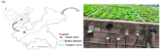
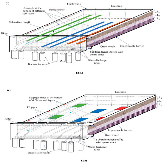
Figure 1.
The location of test plots (a), the layout of the U-trough collection method (UCM) devices (b), and the layout of seepage plate collection method (SPM) devices (c).
2.2. Experimental Design
This research aims to verify the reliability of UCM on soil water, sediment and nutrient migration load at different soil layers (L1: 0–20 cm, L2: 20–40 cm, L3: 40–60 cm), compared to the SPM [53]. The UCM was designed to collect the SSR of a consecutive belt-region from the top slope to the bottom slope, while the SPM was used to collect the SSR of a dot area at the top slope and the bottom slope. As shown in Figure 1b,c, two U-troughs or two seepage plates were installed and fixed at each soil layer’s bottom. Each U-trough was a polyvinyl chloride (PVC) flume with 10 cm width, 5 cm depth, and its length was consistent with the length of the experimental plot. In each plot, the vertical projection spacing of all U-troughs was 40 cm. The vertical projection spacing of all the seepage plates was 70 cm in the transversal slope direction and was 4.5 m in the longitudinal slope direction. All collection devices of the UCM and SPM methods were kept parallel to the slope surface. Both kinds of collection devices were filled with 2–4 mm diameter clean quartz sands and covered by two layers of 200-mesh gauzes to improve the hydraulic conductivity. Moreover, all devices of the UCM were connected to the buckets outside of the downslope by discharge tubes, while all SPM devices were connected to buckets by PE pipes. Total SSR in each test plot, except this part collected by devices, was collected by a subdrain trench stuffed with the quartz sand (2–4 mm) and was drained into a bucket by a water discharge tube. Total SR in each test plot was collected by an open trench and then discharged into a bucket through a discharge tube. Each bucket had nine shunt holes, and one of the shunt holes connected to a sub-bucket through a water pipeline. This research had been conducted with three duplicates of each collection system. Briefly, the corn–mustard rotation, two times of fertilizer applications for summer maize and one-time fertilizer application for winter mustard, was set up in each year in this study. The fertilization was applied at a depth of 5–10 cm to avoid surface loss. This study had been conducted over two consecutive years’ field monitoring.
2.3. Experiment Data Collections and Processing
The volume of each fluid sample was the volume of water in the corresponding bucket of each device. When the collected SSR by the device was more than 1 L, we sampled 1 L and divided it into two 0.5 L for the nutrient and sediment concentration analysis; When the collected SSR by the device was 0.5–1 L, we only sampled 0.5 L for the nutrient concentration analysis; When the collected SSR by the device was less than 0.5 L, we did not sample. When the collected SSR by the device was more than 1 L, we sampled 1 L and divided it into two 0.5 L for the nutrient and sediment concentration analysis; when the collected SSR by the device was 0.5–1 L, we only sampled 0.5 L for the nutrient concentration analysis; when the collected SSR by the device was less than 0.5 L, we did not sample. Each soil layer’s SSR volume per rainfall event and the sampling probability during the test period were calculated as follows:
where R is the SSR volume (L) per rainfall event flowing out the specified layer; r is the collected volume (L) by the device; A is the test plot area (m2); a is the collecting area (m2) of the device; SP is the sampling probability (%), i is the times of rainfall–runoff events that met the minimum sampling requirements (collected SSR volume was more than 0.5L); n is the total rainfall-runoff events during the test period.
In the ith rainfall event, the flux of SSR permeating from each soil layer and its total flux in a specified period could be obtained by these equations as follows:
where is the SSR flux (mm) of the nth soil layer in the ith rainfall event; is the average collected volume (L) of SSR through both devices at the same layer; is the total SSR flux (mm) of the nth soil layer; is the number of rainfall events in a specified period; is the number of soil layers.
The amount of sediment was from each SSR sample by the filtration and drying method [61]. The amount of collected sediment that met the minimum sampling requirement was 1.0 g for sediment nutrient analysis and 10.0 g for the particle size distribution analysis under a single rainfall–runoff event. Otherwise, the total mixed sediment amount of several consecutive rainfall events would be obtained. The following equations could calculate the sediment migration intensities of each soil layer.
where is the sediment migration intensity (t/km2) of the nth soil layer in the ith rainfall event; is the dried weight (g) of sediment in each SSR sample of the nth soil layer; is the total sediment migration intensity (t/km2) of the nth soil layer in a specified period; other parameters have the same meanings as above.
The runoff sample from the inside of the bucket was thoroughly stirred before sampling. The soil nutrient migration intensities were obtained from the following equations.
where is the migration intensity (t/km2) of the jth nutrient at the nth soil layer in the ith rainfall event; is the concentration (mg/L) of the jth nutrient at the nth soil layer; is the total migration intensity (t/km2) of the test grid’s jth nutrient at the nth soil layer in a specified period; other parameters have the same meanings as above.
Hourly meteorological data were from a small-sized automatic collection weather station near the research plots. The average annual precipitation was 1009.2 mm in this study. Notably, during the whole experiment period, 312 rainfall events occurred, but only 51 rainfall–runoff events had been observed and collected. During the first cycle year of the test period, at the L1, L2, and L3 layers, 20, 18, 18 valid rainfall–runoff events in UCM and 16, 11 and 11 valid events in SPM were observed and collected, respectively. While during the second cycle year, at the L1, L2, and L3 layers, 31, 31, 31 valid rainfall–runoff events in UCM and 27, 23, 22 valid events in SPM were observed and collected, respectively. This study only reported results from the concentration and migration intensities of total nitrogen (TN) and total phosphorus (TP). The TN and TP concentrations were determined by the Kjeldahl method and the ammonium-molybdate spectrophotometry method, respectively [62]. The sediment samples were dried in an oven at 105 °C to a constant weight. The sediment particle size distribution (PSD) was determined by the conventional pipette method [61]. The basic physicochemical properties of soil were determined as Yang’s methods [63].
2.4. Statistical Analysis
The IBM SPSS Statistics 25 software was the data analysis tool, while the Graph Pad Prism 8 was the mapping software in this paper. The Pearson Correlation was used for the correlation analysis. The Least Significant Difference (LSD) method at p = 0.05 was performed to elucidate any significant differences. The average data were the results of normalizing to the corresponding numbers of their valid events.
3. Results
3.1. SSR Migration Analysis
Figure 2 presented that the UCM presented significant differences in the collected SSR compared to the SPM. As shown in Figure 2a, in the whole test period, the average collected SSR volumes per rainfall event from the L1, L2, and L3 layers under the UCM were 9.69, 9.74, and 9.97 times of those under the SPM, respectively. Additionally, both methods showed that the deeper the soil layer, the lower volumes were collected from the SSR. Noteworthily, the collected SSR volumes under both methods at the L1 layer were significantly higher than those at the other two layers. Figure 2b shows that the SSR flux from each soil layer presented a significantly positively linear correlation with natural rainfall under both methods. However, the flux from the SPM was more seriously affected by the rainfall. With the increase of rainfall, the SSR leaching from each soil layer increased obviously. The topsoil layer was substantially more affected by the rainfall than the two lower layers.
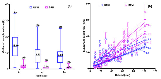
Figure 2.
The collected sample volume (a) and the relationship between subsurface runoff (SSR) flux and rainfall (b) at each soil layer under both methods. The L1, L2, and L3 values represent the SSR flux flowing out of the corresponding soil layer, respectively. The capital letters indicate significant differences between different soil layers, and the lowercase letters indicate significant differences in the same layer between different methods at p = 0.05. The solid line is the best-fit line of simple linear regression, and the dotted lines are the 95% confidence bands. The values in the box plots are the medians.
Table 1 presents that the UCM had significantly higher sampling probabilities at each soil layer than the SPM. The annual sampling probability of collected SSR volume met the minimum sampling requirement reached up to 95.00–100% under the UCM, compared to 63.4–83.00% under the SPM. The annual SSR flux from L1 to L3 was 403.4 mm, 271.9 mm, and 237.4 mm under the UCM, 14.35%, 10.56%, and 8.41% lower than those under the SPM, respectively. The difference between both methods in the annual SSR flux was significant between the L1 and L2 layers. However, it was not significant at the eventual loss flux from the L3 layer. The difference between the infiltrated flux and each soil layer’s outflow flux was the intercepted amount at this layer. The upper soil layer’s outflow flux was the infiltrated flux of the next soil layer. The total permeating water flux through the soil surface (L0) was the difference between the precipitation and SR flux; 57.31%, 16.03%, and 1.53% of annual total permeating water flux (944.9 mm) was retained by the L1, L2, L3 layers under the UCM, respectively. In comparison, the proportions were 50.81%, 17.44%, and 4.68% under the SPM. Briefly, the sharp decrease of SSR flux from L0 to L1 indicated that most of the infiltration flux was intercepted by the L1 layer. The deeper the soil layer, the lower the interception capability of this soil layer.

Table 1.
Annual sampling probability, and SSR, sediment, TN, TP migration loads under the UCM and SPM.
3.2. Sediment Migration Analysis
Figure 3 existed that the difference in sediment migrations under both methods was significant. In Figure 3a, during the test period, the average collected sediment amounts per rainfall event at the L1, L2, and L3 layers under UCM were 6.22, 3.61, 4.97 times those under SPM. The deeper the soil layer, the lower the sediment amount collected. The sediment collected by the SPM was basically less than the minimum sampling requirement of 1.0 g under a single rainfall–runoff event. Figure 3b indicates that each soil layer’s migrated sediment load presented a significantly positively linear correlation with rainfall under both methods. However, when the rainfall was higher than 20 mm, the migrated sediment loads from the SPM at each soil layer were higher and more substantially affected by rainfall. With increased rainfall, the sediment migration amounts at each soil layer increased obviously. The topsoil layer was more obviously affected by rainfall than the two lower layers. Figure 3c indicates that the sediment particle size distribution (PSD) was significantly different in each soil layer. The fine particle with a size less than 0.05 mm dominated the sediment at each soil layer. The cumulative weight percentage of sediment particles below 0.002 mm at L1 was 55.09%, while 86.40% at L2, and 76.48% at L3. Remarkably, the particles’ size at L1 was more extensive than that at other layers, and the L2 layer had the smallest sediment particle.
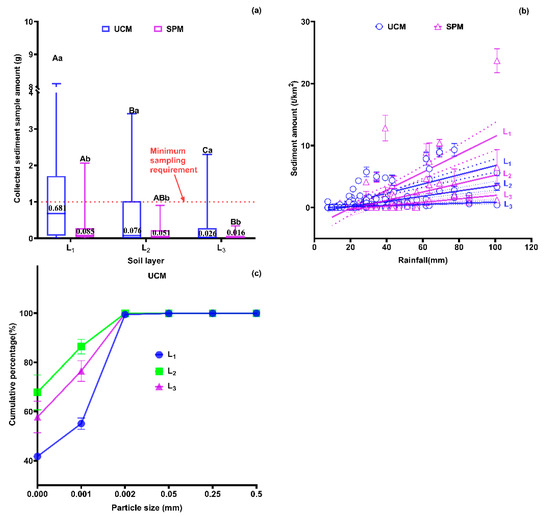
Figure 3.
The collected sediment amount (a), the relationship between sediment amount and rainfall (b) and particle size distribution of sediment (c) at each soil layer under the UCM and SPM. The L1, L2 and L3 values represented the sediment amount migrated out of the corresponding soil layer, respectively. The capital letters indicate significant differences between different soil layers, and the lowercase letters indicate significant differences in the same layer between different methods at p = 0.05. The solid line is the best-fit line of simple linear regression, and the dotted lines are the 95% confidence bands. The values in the box plots are the medians.
The difference of sediment migrating load between the two adjacent layers was the net intercepted amount. As shown in Table 1, the deeper the soil layer, the lower the net intercepted amount. The annual sediment migrating out of the L1 layer was 49.562 t/km2 under UCM, while it was 48.708 t/km2 under SPM. The annual sediment migrating out of the L2 layer under the UCM was 12.475 t/km2, which meant that the L2 layer intercepted 74.83% of the L1 layer’s net leached loss. The annual sediment migrating out of the L3 layer was 6.63 t/km2 under UCM. The L3 layer intercepted 5.845 t/km2 of sediment, accounted for 11.79%, 46.85% of the L1 and L2 layers’ net leached loss, respectively. Though the sediment migrating loads under a single rainfall event were significantly different between the UCM and SPM (shown in Figure 3b), the annual net sediment migrating loads of both methods at each layer had no significant differences. Briefly, 86.62% and 88.24% of the topsoil layer’s leached sediment under the UCM and SPM were withheld by the subsoil layers (L2 and L3), respectively. According to Pearson correlation analysis (shown in Table 2), the different soil layers’ annual sediment migration loads under UCM showed no significant relationship with the annual SSR flux. In contrast, under SPM, they showed a significant relationship.
Table 2.
The correlation analysis of different soil layers’ annual average runoff, sediment, TN and TP migration loads under UCM and SPM.
3.3. Nutrient Migration Analysis
Figure 4 indicated that the difference in nutrient migrations under both methods was not significant. Figure 4a showed that there were no significant differences in TN concentrations between the three soil layers. The average TN concentration under the UCM was 47.43 mg/L at L1, 51.83 mg/L at L2, and 43.28 mg/L at L3, while 50.31 mg/L, 34.83 mg/L, and 51.23 mg/L under the SPM, respectively. Figure 4b indicated that the TN migration amount at each soil layer presented a significantly positively linear correlation with rainfall under the UCM and SPM. However, the TN concentrations from the SPM under the same rainfall event at each soil layer were higher than those from the UCM. In other words, the SPM was more substantially affected by rainfall than the UCM. Figure 4c shows no significant differences in TP concentrations between the L2 and L3 layers, except in the topsoil layer (L1). The average TP concentration under the UCM was 0.71 mg/L at L1, 0.30 mg/L at L2, and 0.22 mg/L at L3, while 0.59 mg/L, 0.29 mg/L, and 0.22 mg/L under the SPM, respectively. Figure 4d indicated that the TP migration amount at each soil layer presented a significantly positively linear correlation with natural rainfall under both ways. However, the TP concentrations from the SPM under the same rainfall event at each soil layer were higher, but not significantly, than those from the UCM.
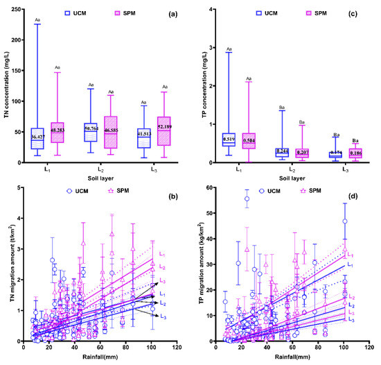
Figure 4.
The TN concentration(a), the relationship between TN migration amount and rainfall (b), and the TP concentration (c), the relationship between TP migration amount and rainfall (d) at each soil layer. The L1, L2, and L3 values are the TN or TP amounts migrated out of the corresponding soil layer, respectively. The capital letters indicate significant differences between different soil layers, and the lowercase letters indicate significant differences in the same layer between different methods at p = 0.05. The solid line is the best-fit line of simple linear regression, and the dotted lines are the 95% confidence bands. The values in the box plots are the medians.
As shown in Table 1, the annual leached TN out of the L1 layer was 19.113 t/km2 under UCM, while it was 22.342 t/km2 under SPM. Under UCM, the annual migrated sediment out of the L2 layer was 13.795 t/km2, namely that the L2 layer intercepted 27.83% of the L1 layer’s leached TN. The L3 layer intercepted 2.558 t/km2 of TN, and accounted for 13.39%, 18.15% of the L1 and L2 layers’ leached TN, respectively. The annual migrated TN loads of both collection methods at each soil layer had no significant difference. Briefly, 41.21% and 53.06% of the topsoil layer’s leached TN under UCM and SPM were withheld by the subsoil layers (L2 and L3), respectively. Note that 58.79%, 46.94% of the L1 layer’s annual leached TN was finally lost from the bottom of the test plot through the SSR. The annual net leached TP out of the L1 layer under the UCM was 0.291 t/km2, while it was 0.286 t/km2 under the SPM. The annual migrated TP out of the L2 layer under the UCM was 0.081 t/km2, which meant a net of 0.210 t/km2 (72.31% of the L1 layer’s annual leached TP) was intercepted by the L2 layer. The L3 layer intercepted 0.028 t/km2 of TP, and accounted for 9.61%, 34.71% of the L1 and L2 layers’ net leached TP loss, respectively. The annual migrated TP loads of both collection systems at each layer presented no significant difference. Also, 81.78% and 80.42% of the topsoil layer’s leached TP under UCM and SPM were withheld by the subsoil layers (L2 and L3), respectively. Only 18.21%, 19.58% of the L1 layer’s annual net leached TP finally lost from the bottom of the test plot through the SSR.
According to Pearson correlation analysis (shown in Table 2), under UCM, the different soil layer’s annual migrated TN loads had no significant relationship with the annual SSR flux but showed significant positive relationships with the annual sediment loads; the different soil layer’s annual migrated TP loads had no significant relationships with the annual sediment loads but showed extremely significant positive relationships with the annual SSR flux. While under SPM, the annual migrated TN loads presented significant relationships with annual SSR flux and extremely significant relationships with the annual sediment loads; the annual migrated TP loads presented significant relationships with annual SSR flux but showed no significant relationship with the annual sediment loads. Additionally, the annual migrated TN loads had no significant relationship with the annual migrated TP loads under UCM but showed significant positive relationships under SPM.
4. Discussion
The difference between the two methods was due to the difference in their collection devices. It was easy to find that the average collected SSR volume and collected sediment amount from the collected devices, SSR and sediment migrating loads per rainfall event were significantly different under UCM and SPM. These differences were rooted in the difference of various devices’ efficient collection areas. In this study, the collecting area of the U-trough was ten times that of the seepage plate. It can be proved in Figure 2a that the average collected SSR volume per rainfall event at each soil layer under UCM was nearly 10 times that under SPM. Undoubtedly, these differences eventually led to the difference in sampling probabilities of both methods. It can be testified in Table 1 that 95.00% of the annual rainfall–runoff events were observed and collected at all soil layers under the UCM, while only 62.99% under the SPM. That is because the SSR flux during some light rainfall events was hard to observe and collect under the SPM. Therefore, the UCM could collect more leakage water from the upper soil layer and be more sensitive to rainfall, especially to the minor rainfall events, than the SPM. The runoff flux, sediment, and nutrient per rainfall event under the SPM were higher than those under the UCM. There might be two reasons as following: firstly, the PE pipe connected to the seepage plate in the soil was empty, which can improve the soil water transmitting ability indirectly; secondly, the lower outlet of the PE pipe was open, then the water in the pipe flowed downward under the gravity might produce negative pressure on the seepage plate and cause a siphonic effect. Therefore, it can accelerate the SSR to flow through the SPM and improve the capability to transport the sediment and nutrient, which can be deduced in Figure 2b, Figure 3b and Figure 4b.
Notably, though the differences in SSR flux per rainfall at each soil layer between the UCM and SPM were significant, the differences in the annual sediment, TN and TP migration loads between the UCM and SPM were not significant. That is because more valid rainfall events were observed and collected under the UCM than those under the SPM, as mentioned above. Thus, the more the total SSR flux could be obtained under UCM to make up the difference. It can be proved in Table 1 that the sampling probabilities under UCM were higher than those under SPM, but the differences in annual sediment, TN and TP migration loads between both methods were not significant. Additionally, compared with the SPM’s point-like layout, the UCM’s collecting area was a continuous area from the top to the slope’s bottom. It might effectively reduce soil heterogeneity of slope, but it still needs more further studies to be proved.
The difference in sediment, SSR, TN and TP migration loads between different soil layers was due to the difference in soil structure characteristics of different soil layers. The topsoil layer was abundant in soil pores [64] and always presented lower moisture than the subsoil layer under the comprehensive affection of gravity and evapotranspiration during the no-rain period. [6,65]. Thus, in the rainy time, the topsoil layer showed high water absorption and storage capacity and absorbed rainfall–runoff firstly to make up soil moisture loss. Then, the SSR in the topsoil layer diffused downward gradually. There might not be enough SSR flux to spread down to the lower layers after the topsoil layer’s interception, especially during some minor rainfall events. The soil pores in the soil can provide preferential flow pathways [66], which might accelerate the nutrient transmitting, especially for phosphorus migrating. That is why the annual leached TN and TP loads from the topsoil layer were quite high, as shown in Table 1. Subsoil with strong adsorption capacity could be considered an appropriate filter to leached nutrients, especially leached phosphorus [66]. The soil subsidence under gravity, leaching and less disturbance made the plow pan soil in a compact structure with fewer soil pores [61,67], which might stop sediment particles of large size from being transmitted downward. It can be proved in Figure 3c. The plow pan soil could intercept most sediment and phosphorus leaching loss of the topsoil [68], which can be proved in Table 1 and Figure 4c. Only a small portion of leached phosphorus was eventually lost, which can be tested in Figure 4c. The detrital shale parent material layer with rich cracks, strong permeability, and weak water-holding capacity [56] would contribute to the sediment, nutrient transmitting. Hence, this layer presented no significant interception ability of leaching sediment and nutrient, which can be seen in Table 1. Additionally, according to Pearson correlation analysis (shown in Table 2), the different soil layers’ annual sediment migration loads showed no significant relationship with the annual SSR flux under UCM but showed significant relationships under SPM. Under UCM, the different soil layers’ annual migrated TN loads showed significant positive relationships with the annual sediment loads; the different soil layer’s annual migrated TP loads showed extremely significant positive relationships with the annual SSR flux. While under SPM, the annual migrated TN loads presented significant relationships with annual SSR flux and extremely significant relationships with the annual sediment loads; the annual migrated TP loads presented significant relationships with annual SSR flux. Additionally, the annual migrated TN loads had no significant relationship with the annual migrated TP loads under UCM but showed significant positive relationships under SPM.
5. Conclusions
The average leached TN, TP concentrations per rainfall event and their annual migrated loads at each soil layer between the SPM and UCM showed no significant difference. Under both methods, the different soil layer’s annual TP migration loads showed significant relationships with the annual SSR. In contrast, the different soil layers’ annual TP migration loads showed significant positive relationships with the annual sediment loads. Both methods also indicated that the topsoil layer was the main layer to retain rainfall–runoff and showed the source of leached sediment and soil nutrient. The subsoil layers, especially the plow pan soil layer, presented a significant interception role of leached sediment and soil nutrients. However, the collecting area of devices significantly affected each soil layer’s sediment, TN and TP migration loads per rainfall event. The U-trough with a larger collecting area could collect higher SSR volume than the seepage plate and keep a higher sampling probability at each soil layer. In conclusion, the UCM was proved to be a reliable quantitative method for subsurface runoff, sediment, and soil nutrient migration loads from diverse soil layers of purple soil sloping cultivated lands. Additionally, we just did the comparison test of both methods in the purple soil sloping cropland in this study, so it needs further studies to testify their availability in other land-use.
6. Patents
The UCM has been applied for an invention patent (application No.: 202010204850.9) in China on 22 March 2020.
Author Contributions
Conceptualization, and methodology, Y.W. and J.N.; writing—original draft preparation, Y.W.; writing—review and editing, C.N. and S.W.; project administration and funding acquisition, J.N. and D.X. All authors have read and agreed to the published version of the manuscript.
Funding
This work was supported by the National Key Research and Development Program of China (grant No. 2018FYD0200701), the National Natural Science Foundation of China (NSFC, 41371275), and the Special Social Livelihood Key R & D Project of Chongqing (cstc2018jscx-mszdx0008).
Data Availability Statement
This study did not report any data.
Acknowledgments
C.N. thanks the support of Bayu Young Scholar from Chongqing, and J.N. acknowledges the support from Chongqing Distinguished Talent.
Conflicts of Interest
The authors declare no conflict of interest.
Abbreviations
The following abbreviations are used in this manuscript:
| UCM | U-trough collection method |
| SPM | Seepage plate collection method |
| SR | Surface runoff |
| SSR | Subsurface runoff |
| SP | Sampling probability |
| TP | Total phosphorus |
| TN | Total nitrogen |
References
- Yang, R.; Tong, J.; Hu, B.X.; Li, J.; Wei, W. Simulating water and nitrogen loss from an irrigated paddy field under continuously flooded condition with Hydrus-1D model. Environ. Sci. Pollut. Res. 2017, 24, 15089–15106. [Google Scholar] [CrossRef]
- Cameron, K.; Di, H.; Moir, J. Nitrogen losses from the soil/plant system: A review. Ann. Appl. Biol. 2013, 162, 145–173. [Google Scholar] [CrossRef]
- Zhu, B.; Wang, T.; Kuang, F.; Luo, Z.; Tang, J.; Xu, T. Measurements of Nitrate Leaching from a Hillslope Cropland in the Central Sichuan Basin, China. Soil Sci. Soc. Am. J. 2009, 73, 1419–1426. [Google Scholar] [CrossRef]
- Freeze, R.A. Reply [to “Comments on ‘Role of subsurface flow in generating surface runoff: 1, Base flow contributions to channel flow’ by R. Allan Freeze”]. Water Resour. Res. 1973, 9, 491. [Google Scholar] [CrossRef]
- Li, J.; Guo, M.; Guo, M.; Kang, H.; Wang, Z.; Huang, J.; Sun, B.; Wang, K.; Zhang, G.; Bai, Y. Effects of soil texture and gravel content on the infiltration and soil loss of spoil heaps under simulated rainfall. J. Soils Sediments 2020, 20, 3896–3908. [Google Scholar] [CrossRef]
- Mohammadzadeh-Habili, J.; Heidarpour, M.; Khalili, D. Effect of Aggregate Size and Porosity of Clay Soils on the Hydraulic Parameters of the Green-Ampt Infiltration Model. J. Hydrol. Eng. 2018, 23, 06018001. [Google Scholar] [CrossRef]
- Cheik, S.; Bottinelli, N.; Sukumar, R.; Jouquet, P. Fungus-growing termite foraging activity increases water infiltration but only slightly and temporally impacts soil physical properties in southern Indian woodlands. Eur. J. Soil Biol. 2018, 89, 20–24. [Google Scholar] [CrossRef]
- Li, B.; Gao, J.; Wang, X.; Ma, L.; Cui, Q.; Vest, M. Effects of biological soil crusts on water infiltration and evaporation Yanchi Ningxia, Maowusu Desert, China. Int. J. Sediment Res. 2016, 31, 311–323. [Google Scholar] [CrossRef]
- Xie, C.; Cai, S.; Yu, B.; Yan, L.; Liang, A.; Che, S. The effects of tree root density on water infiltration in urban soil based on a Ground Penetrating Radar in Shanghai, China. Urban For. Urban Green. 2020, 50, 126648. [Google Scholar] [CrossRef]
- Leung, A.K.; Boldrin, D.; Liang, T.; Wu, Z.Y.; Kamchoom, V.; Bengough, A.G. Plant age effects on soil infiltration rate during early plant establishment. Géotechnique 2017, 68, 1–7. [Google Scholar] [CrossRef]
- Khan, M.N.; Gong, Y.; Hu, T.; Lal, R.; Zheng, J.; Justine, M.F.; Azhar, M.; Che, M.; Zhang, H. Effect of Slope, Rainfall Intensity and Mulch on Erosion and Infiltration under Simulated Rain on Purple Soil of South-Western Sichuan Province, China. Water 2016, 8, 528. [Google Scholar] [CrossRef]
- Huang, J.; Wu, P.; Zhao, X. Effects of rainfall intensity, underlying surface and slope gradient on soil infiltration under simulated rainfall experiments. Catena 2013, 104, 93–102. [Google Scholar] [CrossRef]
- Zhao, L.; Hou, R.; Wu, F.; Keesstra, S. Effect of soil surface roughness on infiltration water, ponding and runoff on tilled soils under rainfall simulation experiments. Soil Tillage Res. 2018, 179, 47–53. [Google Scholar] [CrossRef]
- Zhao, L.; Wang, L.; Liang, X.; Wang, J.; Wu, F. Soil Surface Roughness Effects on Infiltration Process of a Cultivated Slopes on the Loess Plateau of China. Water Resour. Manag. 2013, 27, 4759–4771. [Google Scholar] [CrossRef]
- Jeong, S.; Kim, Y.; Park, H.; Kim, J. Effects of rainfall infiltration and hysteresis on the settlement of shallow foundations in unsaturated soil. Environ. Earth Sci. 2018, 77, 494. [Google Scholar] [CrossRef]
- Bashir, R.; Sharma, J.; Stefaniak, H. Effect of hysteresis of soil-water characteristic curves on infiltration under different climatic conditions. Can. Geotech. J. 2016, 53, 273–284. [Google Scholar] [CrossRef]
- Watanabe, K.; Kugisaki, Y. Effect of macropores on soil freezing and thawing with infiltration. Hydrol. Process. 2017, 31, 270–278. [Google Scholar] [CrossRef]
- Litt, G.F.; Ogden, F.L.; Mojica, A.; Hendrickx, J.M.H.; Kempema, E.W.; Gardner, C.B.; Bretfeld, M.; Regina, J.A.; Harrison, J.B.J.; Cheng, Y.; et al. Land cover effects on soil infiltration capacity measured using plot scale rainfall simulation in steep tropical lowlands of Central Panama. Hydrol. Process. 2020, 34, 878–897. [Google Scholar] [CrossRef]
- Chalise, K.S.; Singh, S.; Wegner, B.R.; Kumar, S.; Pérez-Gutiérrez, J.D.; Osborne, S.L.; Nleya, T.; Guzman, J.; Rohila, J.S. Cover Crops and Returning Residue Impact on Soil Organic Carbon, Bulk Density, Penetration Resistance, Water Retention, Infiltration, and Soybean Yield. Agron. J. 2019, 111, 99–108. [Google Scholar] [CrossRef]
- Negev, I.; Shechter, T.; Shtrasler, L.; Rozenbach, H.; Livne, A. The Effect of Soil Tillage Equipment on the Recharge Capacity of Infiltration Ponds. Water 2020, 12, 541. [Google Scholar] [CrossRef]
- Sithole, N.J.; Magwaza, L.S.; Thibaud, G.R. Long-term impact of no-till conservation agriculture and N-fertilizer on soil aggregate stability, infiltration and distribution of C in different size fractions. Soil Tillage Res. 2019, 190, 147–156. [Google Scholar] [CrossRef]
- He, X.; Zheng, Z.; Li, T.; He, S. Effect of Slope Gradient on Phosphorus Loss from a Sloping Land of Purple Soil under Simulated Rainfall. Pol. J. Environ. Stud. 2020, 29, 1637–1647. [Google Scholar] [CrossRef]
- Zhang, Y.; Xie, D.; Ni, J.; Zeng, X. Optimizing phosphate fertilizer application to reduce nutrient loss in a mustard (Brassica juncea var. tumida)-maize (Zea mays L.) rotation system in Three Gorges Reservoir area. Soil Tillage Res. 2019, 190, 78–85. [Google Scholar] [CrossRef]
- Bosch, D.D.; Truman, C.C.; Potter, T.L.; West, L.T.; Strickland, T.C.; Hubbard, R.K. Tillage and slope position impact on field-scale hydrologic processes in the South Atlantic Coastal Plain. Agric. Water Manag. 2012, 111, 40–52. [Google Scholar] [CrossRef]
- Bosch, D.D.; Potter, T.L.; Strickland, T.C.; Hubbard, R.K. Dissolved Nitrogen, Chloride, and Potassium Loss from Fields in Conventional and Conservation Tillage. Trans. ASABE 2015, 58, 1559–1571. [Google Scholar] [CrossRef]
- Sadhukhan, D.; Qi, Z.; Zhang, T.-Q.; Tan, C.S.; Ma, L. Modeling and Mitigating Phosphorus Losses from a Tile-Drained and Manured Field Using RZWQM2-P. J. Environ. Qual. 2019, 48, 995–1005. [Google Scholar] [CrossRef] [PubMed]
- Singh, S.; Bhattarai, R.; Negm, L.M.; Youssef, M.A.; Pittelkow, C.M. Evaluation of nitrogen loss reduction strategies using DRAINMOD-DSSAT in east-central Illinois. Agric. Water Manag. 2020, 240, 106322. [Google Scholar] [CrossRef]
- Zajíček, A.; Fučík, P.; Kaplická, M.; Liška, M.; Maxová, J.; Dobiáš, J. Pesticide leaching by agricultural drainage in sloping, mid-textured soil conditions—The role of runoff components. Water Sci. Technol. 2018, 77, 1879–1890. [Google Scholar] [CrossRef] [PubMed]
- Manninen, N.; Soinne, H.; Lemola, R.; Hoikkala, L.; Turtola, E. Effects of agricultural land use on dissolved organic carbon and nitrogen in surface runoff and subsurface drainage. Sci. Total. Environ. 2018, 618, 1519–1528. [Google Scholar] [CrossRef]
- Jiang, Q.; Qi, Z.; Lu, C.; Tan, C.S.; Zhang, T.; Prasher, S.O. Evaluating RZ-SHAW model for simulating surface runoff and subsurface tile drainage under regular and controlled drainage with subirrigation in southern Ontario. Agric. Water Manag. 2020, 237, 106179. [Google Scholar] [CrossRef]
- Pisani, O.; Liebert, D.; Bosch, D.; Coffin, A.; Endale, D.; Potter, T.; Strickland, T. Element losses from fields in conventional and conservation tillage in the Atlantic Coastal Plain, Georgia, United States. J. Soil Water Conserv. 2020, 75, 376–386. [Google Scholar] [CrossRef]
- Guo, T.; Gitau, M.; Merwade, V.; Arnold, J.; Srinivasan, R.; Hirschi, M.; Engel, B. Comparison of performance of tile drainage routines in SWAT 2009 and 2012 in an extensively tile-drained watershed in the Midwest. Hydrol. Earth Syst. Sci. 2018, 22, 89–110. [Google Scholar] [CrossRef]
- Bjerkholt, J.T.; Kværner, J.; Jenssen, P.D.; Briseid, T. Mitigating particle and nutrient losses via subsurface agricultural drainage using lightweight aggregates. Agric. Water Manag. 2019, 213, 1004–1015. [Google Scholar] [CrossRef]
- Tao, Y.; Wang, S.; Xu, D.; Yuan, H.; Chen, H. Field and numerical experiment of an improved subsurface drainage system in Huaibei plain. Agric. Water Manag. 2017, 194, 24–32. [Google Scholar] [CrossRef]
- Huang, R.; Gao, X.; Wang, F.; Xu, G.; Long, Y.; Wang, C.; Wang, Z.; Gao, M. Effects of biochar incorporation and fertilizations on nitrogen and phosphorus losses through surface and subsurface flows in a sloping farmland of Entisol. Agric. Ecosyst. Environ. 2020, 300, 106988. [Google Scholar] [CrossRef]
- Deng, L.; Sun, T.; Fei, K.; Zhang, L.; Fan, X.; Wu, Y.; Ni, L. Effects of erosion degree, rainfall intensity and slope gradient on runoff and sediment yield for the bare soils from the weathered granite slopes of SE China. Geomorphology 2020, 352, 106997. [Google Scholar] [CrossRef]
- Deng, L.-Z.; Zhang, L.P.; Sun, T.-Y.; Zhang, L.-P.; Fan, X.-J.; Ni, L. Characteristics of runoff processes and nitrogen loss via surface flow and interflow from weathered granite slopes of Southeast China. J. Mt. Sci. 2019, 16, 1048–1064. [Google Scholar] [CrossRef]
- Deng, L.-Z.; Zhang, L.P.; Sun, T.-Y.; Zhang, L.-P.; Fan, X.-J.; Ni, L. Phosphorus Loss through Overland Flow and Interflow from Bare Weathered Granite Slopes in Southeast China. Sustainability 2019, 11, 4644. [Google Scholar] [CrossRef]
- Tao, W.; Bo, Z.; Fuhong, K. Reducing interflow nitrogen loss from hillslope cropland in a purple soil hilly region in southwestern China. Nutr. Cycl. Agroecosystems 2012, 93, 285–295. [Google Scholar] [CrossRef]
- Wang, T.; Zhu, B. Nitrate loss via overland flow and interflow from a sloped farmland in the hilly area of purple soil, China. Nutr. Cycl. Agroecosystems 2011, 90, 309–319. [Google Scholar] [CrossRef]
- Wang, S.; Feng, X.; Wang, Y.; Zheng, Z.; Li, T.; He, S.; Zhang, X.; Yu, H.; Huang, H.; Liu, T.; et al. Characteristics of nitrogen loss in sloping farmland with purple soil in southwestern China during maize (Zea mays L.) growth stages. Catena 2019, 182, 104169. [Google Scholar] [CrossRef]
- Hua, K.; Zhu, B. Phosphorus loss through surface runoff and leaching in response to the long-term application of different organic amendments on sloping croplands. J. Soils Sediments 2020, 20, 3459–3471. [Google Scholar] [CrossRef]
- Mazur, A. Quantity and Quality of Surface and Subsurface Runoff from an Eroded Loess Slope Used for Agricultural Purposes. Water 2018, 10, 1132. [Google Scholar] [CrossRef]
- Zheng, H.; Liu, Z.; Zuo, J.; Wang, L.; Nie, X. Characteristics of Nitrogen Loss through Surface-Subsurface Flow on Red Soil Slopes of Southeast China. Eurasian Soil Sci. 2017, 50, 1506–1514. [Google Scholar] [CrossRef]
- Liao, K.; Lai, X.; Zhou, Z.; Liu, Y.; Zhu, Q. Uncertainty analysis and ensemble bias-correction method for predicting nitrate leaching in tea garden soils. Agric. Water Manag. 2020, 237, 106182. [Google Scholar] [CrossRef]
- Li, Y.; Šimůnek, J.; Zhang, Z.; Jing, L.; Ni, L. Evaluation of nitrogen balance in a direct-seeded-rice field experiment using Hydrus-1D. Agric. Water Manag. 2015, 148, 213–222. [Google Scholar] [CrossRef]
- Li, Y.; Šimůnek, J.; Jing, L.; Zhang, Z.; Ni, L. Evaluation of water movement and water losses in a direct-seeded-rice field experiment using Hydrus-1D. Agric. Water Manag. 2014, 142, 38–46. [Google Scholar] [CrossRef]
- Biernat, L.; Taube, F.; Vogeler, I.; Reinsch, T.; Kluß, C.; Loges, R. Is organic agriculture in line with the EU-Nitrate directive? On-farm nitrate leaching from organic and conventional arable crop rotations. Agric. Ecosyst. Environ. 2020, 298, 106964. [Google Scholar] [CrossRef]
- Izydorczyk, K.; Michalska-Hejduk, D.; Jarosiewicz, P.; Bydałek, F.; Frątczak, W. Extensive grasslands as an effective measure for nitrate and phosphate reduction from highly polluted subsurface flow—Case studies from Central Poland. Agric. Water Manag. 2018, 203, 240–250. [Google Scholar] [CrossRef]
- Rodrigo-Comino, J.; Brings, C.; Lassu, T.; Iserloh, T.; Senciales, J.M.; Martínez-Murillo, J.F.; Sinoga, J.D.R.; Seeger, M.; Ries, J.B. Rainfall and human activity impacts on soil losses and rill erosion in vineyards (Ruwer Valley, Germany). Solid Earth 2015, 6, 823–837. [Google Scholar] [CrossRef]
- García-Díaz, A.; Bienes, R.; Sastre, B.; Novara, A.; Gristina, L.; Cerdà, A. Nitrogen losses in vineyards under different types of soil groundcover. A field runoff simulator approach in central Spain. Agric. Ecosyst. Environ. 2017, 236, 256–267. [Google Scholar] [CrossRef]
- Pisani, O.; Strickland, T.C.; Hubbard, R.; Bosch, D.; Coffin, A.W.; Endale, D.; Potter, T.L. Soil nitrogen dynamics and leaching under conservation tillage in the Atlantic Coastal Plain, Georgia, United States. J. Soil Water Conserv. 2017, 72, 519–529. [Google Scholar] [CrossRef]
- Zhang, Y.; Xie, D.; Ni, J.; Zeng, X. Conservation tillage practices reduce nitrogen losses in the sloping upland of the Three Gorges Reservoir area: No-till is better than mulch-till. Agric. Ecosyst. Environ. 2020, 300, 107003. [Google Scholar] [CrossRef]
- Hangen, E.; Gerke, H.; Schaaf, W.; Hüttl, R. Assessment of preferential flow processes in a forest-reclaimed lignitic mine soil by multicell sampling of drainage water and three tracers. J. Hydrol. 2005, 303, 16–37. [Google Scholar] [CrossRef]
- Zhong, S.; Han, Z.; Du, J.; Ci, E.; Ni, J.; Xie, D.; Wei, C. Relationships between the lithology of purple rocks and the pedogenesis of purple soils in the Sichuan Basin, China. Sci. Rep. 2019, 9, 1–13. [Google Scholar] [CrossRef] [PubMed]
- Qian, F.; Linyao, D.; Jigen, L.; Bei, S.; Honghu, L.; Jiesheng, H.; Hao, L. Equations for predicting interrill erosion on steep slopes in the Three Gorges Reservoir, China. J. Hydrol. Hydromech. 2020, 68, 51–59. [Google Scholar] [CrossRef]
- Zheng, J.-J.; He, X.-B.; Walling, D.; Zhang, X.-B.; Flanagan, D.; Qi, Y.-Q. Assessing Soil Erosion Rates on Manually-Tilled Hillslopes in the Sichuan Hilly Basin Using 137Cs and 210Pbex Measurements. Pedosphere 2007, 17, 273–283. [Google Scholar] [CrossRef]
- Wang, Y.; Luo, J.; Zheng, Z.; Li, T.; He, S.; Zhang, X.; Wang, Y.; Liu, T. Assessing the contribution of the sediment content and hydraulics parameters to the soil detachment rate using a flume scouring experiment. Catena 2019, 176, 315–323. [Google Scholar] [CrossRef]
- Luo, J.; Zheng, Z.; Li, T.; He, S. The changing dynamics of rill erosion on sloping farmland during the different growth stages of a maize crop. Hydrol. Process. 2019, 33, 76–85. [Google Scholar] [CrossRef]
- He, S.; Qin, F.; Zheng, Z.; Li, T. Changes of soil microrelief and its effect on soil erosion under different rainfall patterns in a laboratory experiment. Catena 2018, 162, 203–215. [Google Scholar] [CrossRef]
- Zuo, F.-L.; Li, X.-Y.; Yang, X.-F.; Wang, Y.; Ma, Y.-J.; Huang, Y.-H.; Wei, C.-F. Soil particle-size distribution and aggregate stability of new reconstructed purple soil affected by soil erosion in overland flow. J. Soils Sediments 2019, 20, 272–283. [Google Scholar] [CrossRef]
- Bouraima, A.-K.; He, B.; Tian, T. Runoff, nitrogen (N) and phosphorus (P) losses from purple slope cropland soil under rating fertilization in Three Gorges Region. Environ. Sci. Pollut. Res. 2016, 23, 4541–4550. [Google Scholar] [CrossRef] [PubMed]
- Yang, J.H.; Wang, C.L.; Dai, H.L. Soil Agrochemical Analysis and Environmental Monitoring; Li, Y., Ed.; China Land Press: Beijing, China, 2008; pp. 18–188. (In Chinese) [Google Scholar]
- Tsai, T.-L.; Jang, W.-S. Deformation effects of porosity variation on soil consolidation caused by groundwater table decline. Environ. Earth Sci. 2013, 72, 829–838. [Google Scholar] [CrossRef]
- Zhu, J. Impact of fractal characteristics on evaporation and infiltration in unsaturated heterogeneous soils. Hydrol. Sci. J. 2020, 65, 1872–1878. [Google Scholar] [CrossRef]
- Steingruber, S.M.; Reinhardt, M.; Wehrli, B. Nutrient transfer from soil to surface waters: Differences between nitrate and phosphate. Aquat. Sci. 2004, 66, 117–122. [Google Scholar] [CrossRef]
- Peng, X.; Shi, D.; Jiang, D.; Wang, S.; Li, Y. Runoff erosion process on different underlying surfaces from disturbed soils in the Three Gorges Reservoir Area, China. Catena 2014, 123, 215–224. [Google Scholar] [CrossRef]
- Makowski, V.; Julich, S.; Feger, K.-H.; Julich, D. Soil Phosphorus Translocation via Preferential Flow Pathways: A Comparison of Two Sites With Different Phosphorus Stocks. Front. For. Glob. Chang. 2020, 3, 48. [Google Scholar] [CrossRef]


Publisher’s Note: MDPI stays neutral with regard to jurisdictional claims in published maps and institutional affiliations. |
© 2021 by the authors. Licensee MDPI, Basel, Switzerland. This article is an open access article distributed under the terms and conditions of the Creative Commons Attribution (CC BY) license (http://creativecommons.org/licenses/by/4.0/).