Towards Personal Financial Sustainability Based on Human Capital Analysis in Korea

Abstract

Financial sustainability for individuals has become more important due to the increase in life expectancy. In personalized lifetime financial planning, human capital is critical for incorporating the life-cycle of individuals. This study focuses on human capital modeling based on features such as education level and working industry, and presents how difference in human capital can affect the optimal asset allocation. By analyzing the Korean labor and income panel survey data, fixed effects regression was performed to model human capital and a portfolio model that maximizes utility of total wealth is solved to optimize the lifetime financial plan. The empirical results show that individuals with human capital that are more correlated with stocks are advised to reduce allocation in stocks.

1. Introduction

According OECD [1], the proportion of the population aged 65 and above increased from 9% in 1960 to 17% in 2017. This proportion is expected to grow to 27% by 2050. The two main reasons for this change are declining fertility rate and increasing life expectancy. For individuals, longer life expectancy is the bigger concern as this can directly affect the quality of life after retirement. In preparation for such a change, the best approach for achieving financial sustainability is to focus on retirement savings [2]. Furthermore, lifetime financial planning allows for effective saving for retirement that meets personalized circumstances and goals. Even though high-net-worth individuals have traditionally received management services from professional financial managers, most individuals are not able to gain access to such services. Thus, there is much need for automated services that can provide financial planning to all individuals, and the objective of this study is to further analyze appropriate models.

The fundamental quantitative model for financial planning is the mean-variance model, which allows analyzing the risk-return tradeoff of investments [3]. Since the seminal work of Markowitz, there have been numerous extensions including portfolio models that reflect various constraints, models focusing on downside risk, robust portfolio models, and multi-period formulations [4,5,6,7]. When applying portfolio models to long-term financial planning such as pensions, it is effective to consider the life-cycle of individuals because the time remaining until retirement affects the optimal allocation in risky assets such as stocks [8,9].

Furthermore, incorporating human capital is especially important in life-cycle financial planning, where human capital refers to economic value of future labor income [10]. Merton [11] introduces labor income in his multi-period portfolio model, and Zanella [12] uses expected labor income for estimating human capital in financial planning. It is also shown in several studies that including human capital in portfolio models directly affects the optimal allocation of financial assets. In particular, the optimal allocation for financial assets that show low correlation with human capital tends to increase since portfolio risk is diversified to human capital as well. Therefore, when human capital is characterized as being a safe asset, the optimal investment in risky assets should go up [13]. It is also recommended to expand investment in risky assets when the majority of capital is composed of human capital [14]. On the other hand, it is advised to manage risk by reducing investment in stocks during periods when human capital shows high relation to shocks in the stock market [15,16].

These studies on financial planning are becoming much more relevant in practice due to the need for securing financial stability after retirement for average individuals who cannot receive human-advising services. This concern that arises from longer life expectancy is particularly alarming in Korea. In the same OECD report that discusses demographic changes, Korea is shown to have the highest projected proportion of population aged 65 and over in 2050 [1]. The rapid change in demography and population aging calls for various ways to prepare for retirement [17,18]. While the value of financial capital is largely dependent on the movement in financial markets, human capital is a component that primarily depends on personal characteristics such as age, education, geographic location, and type of employment. Therefore, detailed analysis on human capital can lead to more personalized lifetime financial planning. The purpose of this study is to apply a lifetime portfolio model that incorporates human capital analysis to the Korean market by analyzing survey data from the Korean Labor and Income Panel Study (KLIPS) for capturing personalized characteristics. Overall, the main contribution is presenting a lifetime financial planning model and a practical application based on a national-level survey to demonstrate how human capital affects life-cycle financial planning.

The remainder of the paper is organized as follows. Section 2 introduces our proposed formulation for estimating human capital and optimizing asset allocation. Section 3 presents the empirical results on human capital analysis, and empirical analysis on financial planning is shown in Section 4. Section 5 concludes the paper.

2. Models for Human Capital and Asset Allocation

For optimizing a life-cycle financial plan, we begin by analyzing panel data of KLIPS for modeling the income process. Then, correlation between the income process and financial asset returns are estimated. Finally, a portfolio optimization model, that maximizes expected utility while taking financial circumstance and risk appetite into account, is solved for finding the ideal financial plan. We extend the life-cycle portfolio model of [19] by utilizing the methods for modeling human capital introduced in [20]. Much emphasis is put on applying this proposed model in Korea by using actual panel survey data.

2.1. Income Process

Fixed effects regression is used for modeling the labor income process in order to take advantage of the KLIPS panel data available in Korea. For simplicity of the analysis, retirement is assumed to occur at age 65. The current age of individuals is assumed to be aged 22, 24, or 26, which represents ages entering the workforce that may depend on the level of education.

The income process can be described as being composed of three components: part that depends on an individual’s characteristics, part that is affected by long-term volatility, and another component affected by short-term shocks [20]. Thus, the income process can be expressed as

$$\log \left(Y_{i,t}\right)=f\left(t, Z_{i,t}\right)+v_{i,t}+{\epsilon }_{i,t}$$

(1)

where $Y_{i,t}$ as the income of individual i at age t, $f\left(t, Z_{i,t}\right)$ is a deterministic function of age t and other individual characteristics expressed as a vector $Z_{i,t}$. In addition, there are two random components in the formulation given by (1), where ${\epsilon }_{i,t}$ represents temporary shock that is normally distributed, $N(0,{\sigma }_{\epsilon }^2)$, and $v_{i,t}$ represent a persistent shock that is further decomposed as the Equation (2),

$$v_{i,t}=v_{i, t-1}+u_{i,t}$$

(2)

where $v_{i,t}$ is dependent on its previous value $v_{i,t-1}$ along with additional shock at time t, $u_{i,t}$, that is uncorrelated with ${\epsilon }_{i,t}$ and follows a normal distribution $N(0,{\sigma }_u^2)$.

2.2. Risk of Income

The risk of income can be estimated from the error of the income process based on the variance decomposition approach [20,21]. Supposing the discrepancy (or error) between actual value $\log \left(Y_{i,t}\right)$ and estimated value $\widehat{f}\left(t,Z_{i,t}\right)$ is defined as $\log (Y_{i,t}^{*})$, as shown in Equation (3),

$$\log (Y_{i,t}^{*})=\log (Y_{i,t})-\widehat{f}\left(t,Z_{i,t}\right).$$

(3)

The difference in error values can be further expressed as

$$r_{i,d}=\log (Y_{i,t+d}^{*})-\log (Y_{i,t}^{*}),d\in \left\{1,\cdots ,21\right\}$$

(4)

where d is the time difference in years, and $r_{i,d}$ represents differences during various durations. Then, based on the definition given by (4), the variance can be decomposed as

$$Var\left(r_{i,d}\right)=d{\sigma }_u^2+2{\sigma }_{\epsilon }^2.$$

(5)

The variances ${\sigma }_u^2$ and ${\sigma }_{\epsilon }^2$ from (5), which reflect persistent and short-term shocks, respectively, can be estimated from OLS regression with two different series of $r_{i,d}$.

Moreover, the relation between income shocks and financial asset returns is critical when including human capital to portfolio models because diversification is achieved through assets with low correlation. The correlation coefficient between income shocks and stock returns can be estimated from the OLS regression of ${\overline{r}}_1$ on the excess return of stocks where ${\overline{r}}_1$ is the cross-sectional sample mean of $r_{i,1}$ across all individuals.

2.3. Portfolio Model

In order to construct optimal portfolios that incorporate both financial and human capital, we solve a portfolio model that maximizes the expected utility of total wealth that includes human capital. The portfolio model given by (6) maximizes expected utility at each stage for finding an optimal life-cycle financial plan, where scenarios are generated by considering the correlation between financial assets and human capital, and geometric Brownian motion is used for modeling assets [19]. For simplicity, the formulation is written as optimizing a portfolio that invests in a risky asset, such as stocks, with expected return ${\mu }_s$ and variance ${\sigma }_s^2$, and a risk-free asset with return $r_f$,

$$\begin{array}{l}\underset{{\omega }_t}{\max }E\left[U\left(W_{t+1}+H_{t+1}\right)\right]\\ \mathrm{s}.\mathrm{t}.W_{t+1}=\left(W_t+h_t-C_t\right)[{\omega }_t{e}^{{\mu }_s-\left(\frac{1}{2}\right){\sigma }_s^2+{\sigma }_s{Z}_s}+\left(1-{\omega }_t\right)e^{r_f}]\\ H_{t+1}={\displaystyle {\displaystyle \sum }_{j=2}^T}{h}_{t+j}{e}^{\left[-\left(j-1\right)\left(r_f+{\eta }_h+{\xi }_h\right)\right]}\end{array}$$

(6)

where $Z_s$ is a random variable that follows a standard normal distribution, t represents age, T is the retirement age (or end of investment horizon), ${\omega }_t$ is the proportion of investment allocated to the risky asset at age t, $W_t$ is the total financial wealth, and $C_t$ is the amount that is spent and not invested. In addition, $h_t$ represents income at age t and $H_t$ is the human capital estimated from income. The key extension from the portfolio formulation in [19] in our formulation (6) is that income is modeled from Equation (1), which allows incorporating personalized human capital.

For discounting future income, ${\xi }_h$ is the discount factor in human capital accounted for illiquidity risk and ${\eta }_h$ is the risk premium for the income process that can be computed as Equation (7),

$$\begin{array}{c}{\eta }_h=\frac{Cov\left(Z_h, Z_s\right)}{Var\left(Z_s\right)}\left({\mu }_s-r_f\right)\\ =\rho \left[{\mu }_s-\left(e^{r_f}-1\right)\right]\frac{{\sigma }_h}{{\sigma }_s}\end{array}$$

(7)

where ${\sigma }_h$ is the standard deviation of income, $\rho$ is the correlation between income and the risky asset, and $Z_h$ follows a standard normal distribution.

As for the utility function, constant relative risk aversion utility is used as given by Equation (8),

$$\begin{array}{c}U=\frac{{\left(W_{x+1}+H_{x+1}\right)}^{1-\gamma }}{1-\gamma }, \gamma \ne 1\hfill \\ U=\ln \left(W_{x+1}+H_{x+1}\right), \gamma =1\hfill \end{array}$$

(8)

where the relative risk aversion $\gamma$ takes values greater than zero. In our empirical analysis, the expected utility is computed from scenarios generated using Monte Carlo simulation.

3. Human Capital Analysis

3.1. Income Data

The panel survey data KLIPS published by Korea Labor Institute are used for applying the human capital and portfolio models to actual data on individual characteristics and income information. The panel study is the first and the largest domestic panel survey on labor-related topics in Korea. It was initiated in 1998 with 5000 households and the survey includes a wide range of details such as education, unemployment experience, childcare, income, consumption, and retirement. In our analysis, panel data of 21 years from 1998 to 2018 are used and the size of the data is shown in

Table 1. Korean Labor and Income Panel Study (KLIPS) data summary from 1998 to 2018.

Survey Number	Year	Number of Households	Number of Individuals
1	1998	5000	13,321
2	1999	4507	12,037
3	2000	4266	11,205
4	2001	4248	11,051
5	2002	4298	10,966
6	2003	4592	11,541
7	2004	4761	11,660
8	2005	4849	11,580
9	2006	5001	11,756
10	2007	5069	11,855
11	2008	5116	11,734
12	2009	6721	14,489
13	2010	6683	14,118
14	2011	6686	13,899
15	2012	6753	13,998
16	2013	6785	13,887
17	2014	6838	13,168
18	2015	6934	14,011
19	2016	7012	14,202
20	2017	7066	14,475
21	2018	7090	14,444

.

We preprocessed household and individual responses within KLIPS for collecting labor income, financial income, and pension income. These three types of income are combined per household and characteristics of the head of the household are used for fixed effects analysis. In Section 3.2, we primarily used education level and working industry for the following reasons. First, education and industry are two well-known factors that affect labor income. Second, both are objective characteristics of individuals compared to variables such as income satisfaction or health which may be subjective. Finally, education and industry details were provided by most respondents while other variables contained many missing values.

In our analysis, we use household data with male household heads because the number of female household heads is too small for investigating the fixed effects of gender. Furthermore, once missing data and no responses are removed, income data are adjusted for inflation and expressed as values in 1998.

3.2. Fixed Effects Analysis

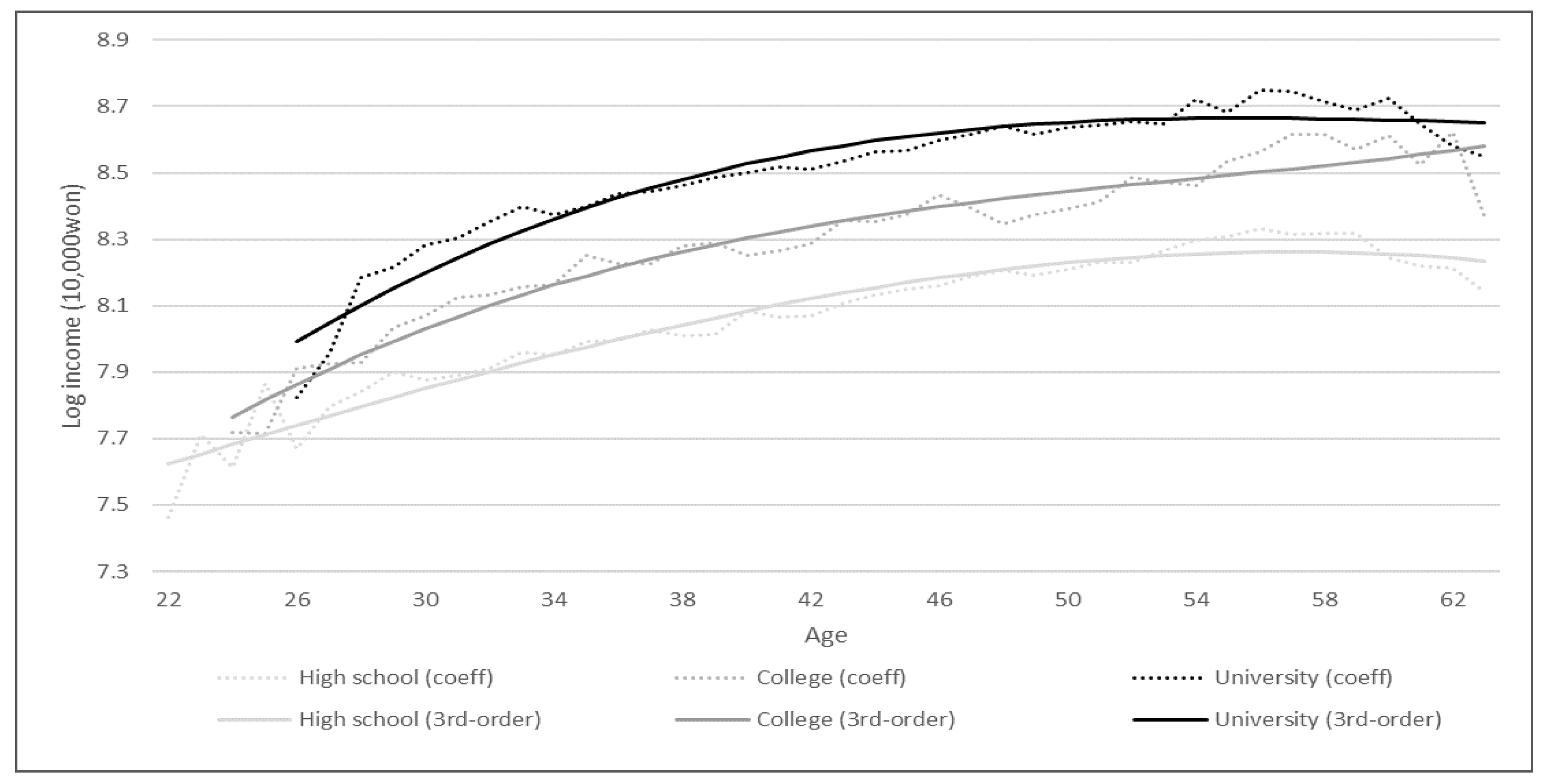
3.2.1. Fixed Effects Regression by Education

We begin by analyzing the effects of education because the importance of higher education is widely acknowledged in Korea [22,23]. In our analysis, education level is divided into three groups: individuals with highest degree in high school, college (or community college), and university (including graduate programs). Lower education levels are not considered because the number of data are too small for performing regression analysis.

For each education group, fixed effects regression model as shown in (9) is performed,

$$\begin{array}{c}\log \left(Y_{i,t}\right)={\beta }_0+{\beta }_1{X}_{i,t}+{\beta }_2{Z}_i+{\epsilon }_{i,t}\\ \mathrm{for}t=1,\cdots ,T \mathrm{and}i=1,\cdots ,N\end{array}$$

(9)

where the dependent variable is the logarithm of income, vector $X_{i,t}$ contains the dummy variables for age, vector $Z_i$ includes fixed effects variables representing marriage status and family size, $\beta$’s are the coefficients, and ${\epsilon }_{i,t}$ is the error term. The results from the fixed effects regression are presented in

Table 2. Fixed effects regression analysis on income.

		High School	College	University
Coeff.	Intercept	7.507 ***	7.802 ***	7.872 ***
	Family size	0.059 ***	0.051 ***	0.044 ***
	Marital status	0.320 ***	0.255 ***	0.384 ***
Sample size		23,510	7388	16,218
R2		0.122	0.171	0.146
Adj. R2		0.121	0.167	0.143
F-statistic		74.24	36.17	68.88

*** p < 0.01.

. We present results when using marital status and family size as fixed effects because these are the key variables describing life-cycle details, in addition to age, and other variables contain too much missing data for performing statistical analysis.

Based on the age dummy variables from regression analysis, the relationship between age and income is shown in Figure 1. The separation among the three education groups is apparent. Income generally increases gradually but may slightly reduce near retirement age. Moreover, based on these results, the age dummy variables can be used to fit a polynomial model for the income process as shown in Figure 1. A polynomial reduces spikes in the estimation of income and a third-order polynomial is used because higher orders do not add much value. Spikes in the estimations for young age from regression are due to limited sample size for this age group but polynomial fitting makes it more appropriate for use in portfolio models. The coefficients of the age polynomials are shown in

Table 3. Third-order polynomial estimation on income.

	High School	College	University
Intercept	−1.177	−3.003	−3.253
Age	0.029	0.148	0.170
Age2/10	0.002	−0.026	−0.027
Age3/100	−0.001	0.002	0.001
R2	0.937	0.939	0.923
Adj. R2	0.932	0.934	0.917

for the three education groups. Variables for age² and age³ are scaled for ease of interpretation.

Finally, variance decomposition of income risk as described in Equation (5) as well as correlation between income and stock returns are estimated as shown in

Table 4. Estimation on income risk and correlation with stocks.

	High School	College	University
${\sigma }_{\epsilon }^2$	0.175 ***	0.146 ***	0.141 ***
${\sigma }_u^2$	0.005 ***	0.010 ***	0.005 ***
ρ	0.633 **	0.335	−0.011 **

*** p < 0.01, ** p < 0.05.

. It shows that individuals with high school degrees have the highest income risk and highest correlation with stocks, whereas individuals with university (or graduate level) degrees have the lowest risk and lowest correlation with stocks. Specifically, the higher risk for high school degree holders is due to high temporary shock ${\sigma }_{\epsilon }^2$. Overall, the low correlation between income of university degree holders and stock returns reflects how having a higher degree leads to jobs that are less affected by the stock market or economic cycles. We later show how this is directly reflected in optimal portfolio allocations.

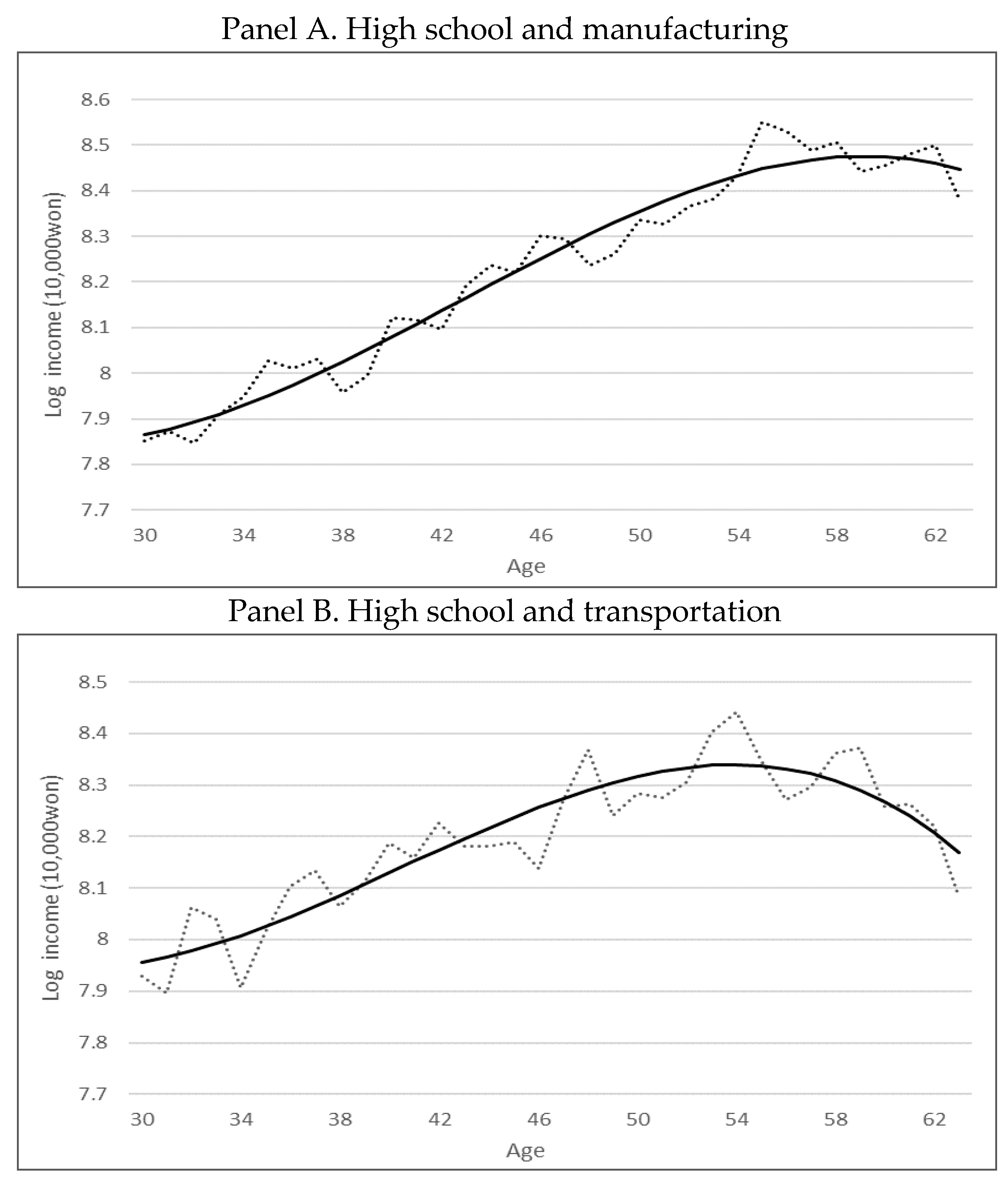
3.2.2. Fixed Effects Regression by Education and Industry

Next, we further personalize individuals by grouping data based on working industry in addition to education levels. It is known that human capital could differ based on industry [24]. Therefore, we categorize individuals into 15 industries and further to three education levels within each industry group. Then, we perform the fixed effects regression analysis presented in Section 3.2.1.

Among the 15 industries, income processes for manufacturing and transportation are further discussed. In

Table 5. Estimation on income risk and correlation with stocks.

	Manufacturing			Transportation
	High School	College	University	High School	College	University
Intercept	8.167 ***	7.996 ***	8.243 ***	7.623 ***	7.707 ***	7.815 ***
Family size	0.068 ***	0.082 ***	0.007	0.053 ***	0.043	0.039
Marital status	0.225 ***	0.210 ***	0.351 ***	0.416 ***	0.556 ***	0.232 **
Age poly. intercept	1.320	2.238	−1.942	1.558	−5.920***	5.703
Age	−0.171 **	−0.205	0.079	−0.167 *	0.353 ***	−0.425 *
Age2/10	0.047 ***	0.054	−0.008	0.046 **	−0.069 **	0.106 *
Age3/100	−0.004 ***	−0.004 *	0.000	−0.004 **	0.005 **	−0.008 **

*** p < 0.01, ** p < 0.05, * p < 0.1.

and

Table 6. Variance decomposition of income for manufacturing and transportation.

	Manufacturing			Transportation
	High School	College	University	High School	College	University
${\sigma }_{\epsilon }^2$	0.129 ***	0.132 ***	0.099 ***	0.110 ***	0.105 ***	0.103 ***
${\sigma }_u^2$	0.006 ***	0.004	0.004 ***	0.004 ***	0.001	0.000

*** p < 0.01.

, results for a total of six groups are shown. Even though some results are not statistically significant because dividing the data into more groups reduces the sample size in each group, it can be clearly realized that the industry has a more noticeable effect on regression and risk decomposition than when only considering education level. For example, marital status is highly significant in all cases and the values show clear difference. As for risk, results for the transportation industry show a steady increase from highest to lowest education level. For the manufacturing industry, the risk between high school and college groups appear to be similar.

The age polynomials presented in Figure 2 also display a difference between the two industries. While both results are for high school degree holders, the transportation industry has lower maximum income level and a steeper decrease near retirement age. The third-order polynomial estimation becomes more valuable in this case because the reduced sample size creates more spikes in the age coefficients from the regression. These distinctions between different industries support the benefit in incorporating background information of individuals in modeling human capital.

4. Life-Cycle Asset Allocation

Glide paths in lifetime financial planning typically refer to reduced allocation in risky assets as retirement approaches [9,25]. Therefore, we also investigate this glide path proportion invested in risky and risk-free assets, but focus on how the personalized glide paths differ for individuals with different human capital, due to varying background characteristics. The annualized mean and standard deviation of the two assets, as shown in

Table 7. Risky and risk-free assets.

	Risky Asset	Risk-Free Asset
Annualized mean	11%	4%
Annualized std. dev.	24%	-

, are computed from historical monthly returns of KOSPI index (Korea Composite Stock Price Index) and the Korea Treasury Bond index during the same period as the KLIPS survey, from 1998 to 2018. While the change in the value of bond indices is perceived as investment risk, we assume that the risk-free asset has zero volatility, which represents cash holdings or long-term treasury holdings in practice.

The optimal lifetime asset allocation is computed by solving the formulation given by (6) for each year starting at the current age. Thus, the optimal allocation in risky and risk-free assets are optimized for each year by modeling the changes in value of financial assets and human capital, which are performed using Monte Carlo simulation. The average portfolio return from the scenarios are used for optimizing the allocation in the following year.

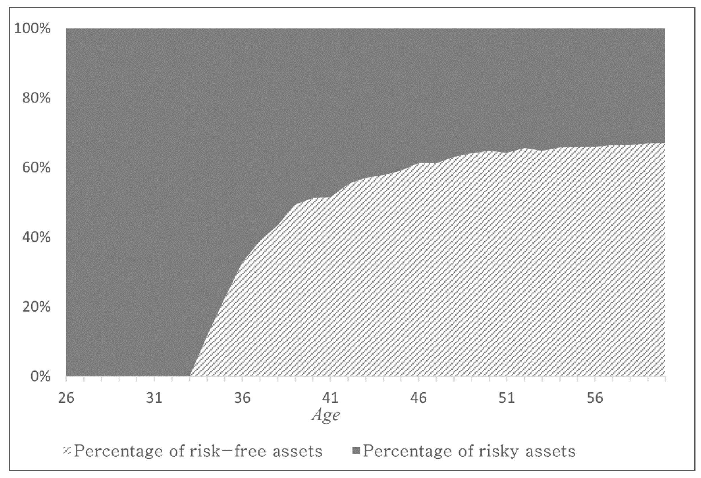
4.1. Asset Allocation Based on Education Level

Figure 3 shows the lifetime asset allocation for individuals with high school degrees. This represents a general glide path where large allocations in the risky asset in early years are followed by a gradual decrease during their lifetime. Even though Figure 3 is the case for a moderate risk level (γ = 4), it shows that full allocation in the risky asset is optimal for the first few years. Investment in risky assets for young investors is generally recommended because there is still enough time to recover from early risky investments, but these results show full exposure in risky assets in the beginning. This is due to the fact that the model is considering human capital as part of total wealth, so there actually is allocation in safer human capital. It is worth recalling that the risk aversion level can be reflected through the utility function as given by (8).

A comparison among the three education groups are summarized in

Table 8. Optimal weights by education level.

	High School		College		University
Age	Risky Asset	Risk-Free Asset	Risky Asset	Risk-Free Asset	Risky Asset	Risk-Free Asset
26	100%	-	100%	-	100%	-
30	100%	-	100%	-	100%	-
34	88.34%	11.66%	97.04%	2.96%	100%	-
35	77.44%	22.56%	83.81%	16.19%	89.29%	10.71%
40	48.75%	51.53%	50.50%	49.50%	51.89%	48.11%
45	40.80%	59.20%	41.53%	58.47%	41.98%	58.02%
50	35.13%	64.87%	35.51%	64.49%	35.73%	64.27%
55	34.16%	65.84%	34.37%	65.63%	34.48%	65.52%
60	33.01%	66.99%	32.99%	67.01%	32.99%	67.01%

. First, it is easily noticeable that large allocation in the risky asset is common for all education levels and decreases with age. More importantly, the difference in correlation between human capital and the risky asset is reflected in the optimal allocation. Human capital for high school graduates has the highest correlation with the returns of stocks, and Table 8 shows that the allocation in the risk-free asset first occurs the earliest for the high school group. The high correlation makes the optimizer consider human capital to be similar to the risky asset, and, thus, increasing the portion invested in the risk-free asset.

On the other hand, it is optimal for individuals with university degrees to be fully invested in the risky asset until aged 35 because large human capital in early years is considered to behave more like the risk-free asset. The allocation for the college group appears to fall between the other two groups as the correlation with stocks was also in the middle.

The portfolio model as given by (6) can also be solved for various risk levels where the risk aversion level is entered through the utility function. Figure 4 shows the optimal lifetime asset allocation for four levels of risk. When γ = 2, which is the least risk-averse case in Figure 4, large investment in the risky asset throughout the entire horizon is shown. In contrast, for the most risk-averse case when γ = 8, it is optimal to start investing earlier in the risk-free asset. The maximum allocation in the risk-free asset reaches 80%, which is the highest among the four cases.

Normally, optimal allocation from portfolio models differ due to varying levels of the investors‘ risk aversion. Nonetheless, the portfolio model based on human capital analysis used in this study not only incorporates personal preference on risk appetite but also adds another level of personalization based on human capital that can capture risk capacity of individuals based on their situation. This personalization through human capital analysis is the key contribution of the model. Next, we observe the case when adding one more layer of personal information.

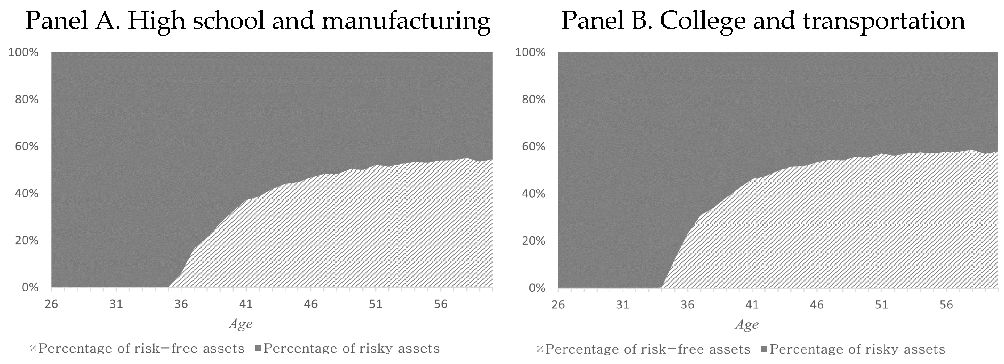
4.2. Asset Allocation Based on Education and Industry

In addition to categorizing individuals based on education levels, we demonstrate further personalization based on two dimensions: education level and job industry. An individual’s job sector is another key factor in optimizing a lifetime financial plan because it has been shown that human capital is affected by industry [24,26]. Moreover, an individual’s labor income may be correlated with the stock market sector of the same industry and less correlated with other sectors, which will have an effect on the optimal portfolio. As shown in

Table 9. Correlation between stocks and various industries.

	High School	College	University
Construction	0.653	0.283	0.030
Educational service	0.495	0.331	0.057
Agriculture, forestry and fisheries	0.600	0.516	0.086
Real estate and rental	0.109	0.041	0.084
Accommodation and restaurant business	0.216	0.273	−0.321
Transportation	0.576	0.238	0.071
Manufacturing	0.086	0.011	0.110

for seven industries as an example, the correlation between stock market returns and various industries can differ widely.

We use transportation and manufacturing to illustrate how the job industry can affect optimal lifetime asset allocation. The Panel A of Figure 5 shows the glide path for an individual with a high school degree that works in the manufacturing industry. Manufacturing is one of the major industries in Korea, so this case would be a relatively common one. Since manufacturing shows a low correlation of less than 0.1 in Table 9, the optimal portfolio contains heavy investment in the risky asset. Full allocation in the risky asset is recommended until the mid-30s and above 40% is optimal even in the 40s. Notably, the correlation for this case is less than the correlation for the entire high school group, so allocation in the risky asset for high school degree holders in manufacturing is much greater than that of Figure 3. This is especially meaningful because we were able to find a financial plan that is more suitable with additional information on human capital. Even though we only include analysis with two dimensions, education level and industry, further customization would be possible if more dimensions (features) are considered.

The case for college graduates working in transportation is shown in Panel B of Figure 5. The correlation for this case is 0.238, which is higher than the case for high school and manufacturing, so the optimal asset allocation contains more investment in the risk-free asset. Larger allocation in the risky asset is optimal compared to the allocation for the college group in Table 8. This is a result of lower correlation for college and transportation group compared to the overall college group. The actual weights are summarized in

Table 10. Optimal weights for two education and industry groups.

	High School & Manufacturing		College & Transportation
Age	Risky Asset	Risk-Free Asset	Risky Asset	Risk-Free Asset
26	100%	-	100%	-
30	100%	-	100%	-
34	100%	-	99.77%	0.23%
35	100%	-	87.98%	12.02%
36	94.10%	5.90%	77.07%	22.93%
40	67.65%	32.35%	57.56%	42.44%
45	55.29%	44.71%	48.25%	51.75%
50	49.96%	50.04%	44.62%	55.38%
55	46.93%	53.07%	42.82%	57.18%
60	45.47%	54.53%	42.03%	57.97%

where a moderate risk level of γ = 4 is assumed.

5. Conclusions

This study addresses the growing concern of personal financial stability due to increased life expectancy by discussing models for life-cycle financial planning. Generally, models for individual lifetime investments such as pensions incorporate investors’ age because investment horizon affects the optimal proportion invested in risky assets (risky assets such as stocks have less risk in the long term and longer investment horizon allows time to recovery from early risky investments). However, as individuals come from various financial and personal backgrounds, further personalization becomes important for constructing an effective lifetime financial plan.

In this study, more dimensions of personal characteristics, in addition to age, are considered for improving human capital estimation. We use the panel survey data of Korea in order to perform a practical analysis on how actual panel data can be used for recommending life-cycle financial plans. In particular, our results from fixed effects regression show that personalized human capital can be modeled by categorizing individuals based on education level and working industry. Moreover, segmentation based on such variables allows for more detailed estimation of correlation with financial assets. For example, individuals with high school degrees tend to have the highest income risk and highest correlation with stocks but the magnitude of difference compared to higher education levels is also dependent on the industry. More importantly, estimated human capital and asset correlation are shown to have a direct effect on optimal life-cycle asset allocation when solving a portfolio model that maximizes the expected total wealth. Individuals with human capital that are more correlated with stocks can reduce the portion of financial wealth invested in stocks, whereas individuals with human capital that show similarity with safe assets can increase investment in stocks. We also show that an individual’s risk aversion can be incorporated in the portfolio model that provides further customization in addition to human capital. These findings clearly show that human capital should be modeled by considering personal situations, which can be modeled from survey data.

We believe that further customization could be possible with a larger dataset. We focused on categorizing individuals based on education level and industry because testing with additional features did not show any statistically significant improvement due to limited responses. The KLIPS data are a nation-wide panel study and one of the largest studies on labor details, but it is a survey-based study that by nature contains missing data. For practical purposes, we believe data preprocessing could resolve some missing data issues by applying basic assumption on lifestyle and family status.

Finally, we note that further studies using other labor-related data could reveal interesting results based on features such as gender, health, and cultural components. It will also be interesting to apply the analysis to countries such as Italy, Portugal, Greece, and Japan, which are OECD countries along with Korea, with expected proportion of population aged 65 and over exceeding one-third by 2050 [1].

References

1. OECD. Health at a Glance 2019: OECD Indicators; OECD Publishing: Paris, France, 2019. [Google Scholar] [CrossRef]
2. Han, J.; Ko, D.; Choe, H. Classifying retirement preparation planners and doers: A multi-country study. Sustainability 2019, 11, 2815. [Google Scholar] [CrossRef] [Green Version]
3. Markowitz, H.M. Portfolio selection. J. Financ. 1952, 7, 77–91. [Google Scholar]
4. Fabozzi, F.J.; Gupta, F.; Markowitz, H.M. The legacy of modern portfolio theory. J. Investig. 2002, 11, 7–22. [Google Scholar] [CrossRef] [Green Version]
5. Kolm, P.N.; Tütüncü, R.; Fabozzi, F.J. 60 Years of portfolio optimization: Practical challenges and current trends. Eur. J. Oper. Res. 2014, 234, 356–371. [Google Scholar] [CrossRef]
6. Kim, W.C.; Kim, J.H.; Fabozzi, F.J. Robust Equity Portfolio Management + Website: Formulations, Implementations, and Properties Using MATLAB; John Wiley & Sons: Hoboken, NJ, USA, 2015. [Google Scholar]
7. Lee, Y.; Kim, W.C.; Kim, J.H. Achieving portfolio diversification for individuals with low financial sustainability. Sustainability 2020, 12, 7073. [Google Scholar] [CrossRef]
8. Modigliani, F. The life cycle hypothesis of saving, the demand for wealth and the supply of capital. Soc. Res. 1966, 33, 160–217. [Google Scholar]
9. Kritzman, M. Target-date funds: A regime-based approach. J. Retire. 2017, 5, 96–105. [Google Scholar] [CrossRef]
10. Mincer, J. Investment in human capital and personal income distribution. J. Political Econ. 1958, 66, 281–302. [Google Scholar] [CrossRef]
11. Merton, R.C. Optimum consumption and portfolio rules in a continuous-time model. J. Econ. Theory 1971, 3, 373–413. [Google Scholar] [CrossRef] [Green Version]
12. Zanella, N. Risk Capacity over the Life Cycle: The Role of Human Capital, High Priority Goals, and Discretionary Wealth. J. Wealth Manag. 2015, 18, 27. [Google Scholar] [CrossRef]
13. Bodie, Z.; Merton, R.C.; Samuelson, W.F. Labor supply flexibility and portfolio choice in a life cycle model. J. Econ. Dyn. Control 1992, 16, 427–449. [Google Scholar] [CrossRef] [Green Version]
14. Heaton, J.; Lucas, D. Market frictions, savings behavior, and portfolio choice. Macroecon. Dyn. 1997, 1, 76–101. [Google Scholar] [CrossRef]
15. Viceira, L.M. Optimal portfolio choice for long-horizon investors with nontradable labor income. J. Financ. 2001, 56, 433–470. [Google Scholar] [CrossRef]
16. Benzoni, L.; Collin-Dufresne, P.; Goldstein, R.S. Portfolio choice over the life-cycle when the stock and labor markets are cointegrated. J. Financ. 2007, 62, 2123–2167. [Google Scholar] [CrossRef]
17. Kim, K.; Yoo, K. Impact of Aging on Household Finance Behavior: Analysis Using the OECD National Panel; KIF Working Paper; Korea Institute of Finance: Seoul, Korea, 2014; pp. 1–57. [Google Scholar]
18. Jeong, W.; Kim, M. Activation of Lifetime Asset Management Service in response to aging population. Korea Insur. Res. Inst. 2015, 2015, 1–91. [Google Scholar]
19. Ibbotson, R.G.; Milevsky, M.A.; Chen, P.; Zhu, K.X. Lifetime Financial Advice: Human Capital, Asset Allocation, and Insurance; The Research Foundation of CFA Institute: Charlottesville, VA, USA, 2007; pp. 1–103. [Google Scholar]
20. Cocco, J.F.; Gomes, F.J.; Maenhout, P.J. Consumption and portfolio choice over the life cycle. Rev. Financ. Stud. 2005, 18, 491–533. [Google Scholar] [CrossRef]
21. Carroll, C.D.; Samwick, A. The Nature of Precautionary Wealth. J. Monet. Econ. 1997, 40, 41–72. [Google Scholar] [CrossRef] [Green Version]
22. Chae, J.E.; Hong, H.K. The expansion of higher education led by private universities in Korea. Asia Pac. J. Educ. 2009, 29, 341–355. [Google Scholar] [CrossRef]
23. Yoon, J.; Park, S.; Kim, D.J. Assessing the Effects of Higher-Education Factors on the Job Satisfaction of Engineering Graduates in Korea. Sustainability 2020, 12, 3342. [Google Scholar] [CrossRef] [Green Version]
24. Weinberg, B.A. Long-term wage fluctuations with industry-specific human capital. J. Labor Econ. 2001, 19, 231–264. [Google Scholar] [CrossRef]
25. Estrada, J. The retirement Glidepath: An international perspective. J. Investig. 2016, 25, 28–54. [Google Scholar] [CrossRef]
26. Neal, D. Industry-specific human capital: Evidence from displaced workers. J. Labor Econ. 1995, 13, 653–677. [Google Scholar] [CrossRef] [Green Version]
Figure 1. Third-order polynomial estimation for income.
Sustainability 13 02700 g001
Figure 2. Age polynomial for high school and two industries.
Sustainability 13 02700 g002
Figure 3. Asset allocation for high school graduates.
Sustainability 13 02700 g003
Figure 4. Asset allocation for several levels of risk aversion.
Sustainability 13 02700 g004
Figure 5. Asset allocation for two education and industry groups.
Sustainability 13 02700 g005