Empirical Characterization Factors for Life Cycle Assessment of the Impacts of Reservoir Occupation on Macroinvertebrate Richness across the United States

Abstract

The transformation of a river into a reservoir and the subsequent occupation of the riverbed by a reservoir can impact freshwater ecosystems and their biodiversity. We used the National Lake Assessment (134 reservoirs) and the National Rivers and Streams Assessment (2062 rivers and streams) of the United States Environmental Protection Agency in order to develop empirical characterization factors (CFs; in Potentially Disappeared Fraction of species [PDF]) evaluating the impacts of reservoir occupation on macroinvertebrate richness (number of taxa) at the reservoir, ecoregion and country spatial scales, using a space-for-time substitution. We used analyses of variance, variation partitioning, and multiple regression analysis to explain the role of ecoregion (or regionalization; accounting for spatial variability) and other potentially influential variables (physical, chemical and human), on PDFs. At the United States scale, 28% of macroinvertebrate taxa disappeared during reservoir occupation and PDFs followed a longitudinal gradient across ecoregions, where PDFs were higher in the west. We also observed that high elevation, oligotrophic and large reservoirs had high PDF. This study provides the first empirical macroinvertebrate-based PDFs for reservoir occupation to be used as CFs by LCA practitioners. The results provide strong support for regionalization and a simple empirical model for LCA modelers.

1. Introduction

Water abstraction (withdrawal), regulation of water flow by dams (storage reservoirs for drinking water, flood control, and energy production), and water diversion by channels (irrigation and navigation) have benefited human populations worldwide [1,2,3]. However, despite clear societal benefits, the use of water is often accompanied by a myriad of environmental impacts [4,5,6,7,8].

The environmental impacts brought about by dams are well documented [9]. Geomorphology, water depth and hydrological regime are notably altered. Changes in water depth, temperature and total dissolved solids affect ecosystem productivity [10,11,12,13]. A change in the hydrological regime (lotic into a lentic ecosystem, upstream of the dam) affects several physical and biological processes, as well as organisms’ capacities to thrive and survive in these ecosystems. These changes can ultimately impact ecosystem biodiversity, productivity and the provision of ecosystem services [14,15,16]. To sustain these services and preserve the ecological integrity of our freshwater ecosystems, we must understand the impacts of dams and reservoirs on freshwater biodiversity. In this article, we are interested in macroinvertebrate richness (number of taxa).

Few studies have investigated the impacts of dams and reservoirs on macroinvertebrate taxa richness. Flow regulation and water level fluctuations (also known as drawdown) [17,18,19,20,21,22] can negatively impact macroinvertebrate richness [23,24,25,26]. However, Glowacki et al. [27] and Floss et al. [28] observed higher taxa richness downstream of a dam, or in regulated rivers, as opposed to natural ones [29]. Marchetti et al. [30] found little difference between richness in reduced flows versus higher “natural-like” flows. The literature highlights divergent macroinvertebrate responses to altered flows.

While the impact of dams and reservoirs on macroinvertebrate richness is an interesting subject on its own, in this article, we are interested in integrating these impacts into an engineering tool that helps decision making (Life Cycle Assessment; LCA). This work specifically aims to assess the potential loss of macroinvertebrates due to dams and reservoirs for multiple usages (hydropower, flood control, irrigation, drinking water, transportation or recreation). For example, in the case of hydropower, we would quantify how many macroinvertebrates would potentially be lost following the implementation of a dam and the creation of a reservoir (transformation from a river into a reservoir and the occupation of the former riverbed by a reservoir) compared to a natural reference and use this information to relate this loss to the kilowatt-hour produced.

LCA is an interdisciplinary and internationally used approach that evaluates the potential environmental impacts of a product, process or service throughout its entire life cycle from resource extraction to end of life [31]. LCA is often used to support the selection of environmentally preferable alternatives for eco-design purposes and to identify the largest potential environmental impacts and trade-offs in a product’s life cycle [32]. Emissions, resource extraction and change in land use (inventory flows) related to all activities involved in the life cycle of a product, process or service are first inventoried, and this is called the Life Cycle Inventory (LCI). Then, these inventory flows are translated into potential environmental impacts through characterization factors (CFs) [33]. In other words, CFs are used to translate inventory flows into impact indicators. Impact indicators are then attributed to Areas of Protection (AoP), which traditionally include ecosystem quality, human health, and resources and ecosystem services [34]. Life Cycle Impact Assessment (LCIA) is the characterization and attribution of the impact. For the ecosystem quality AoP, the use of Potentially Disappeared Fraction of species (PDF), which can also account for time and space, is recommended as a robust impact indicator [34].

The impacts of the transformation of a river into a reservoir (and its subsequent occupation by the reservoir, for a given amount of time) on ecosystem quality have received little attention in LCA. To our knowledge, only a few attempts have been made to evaluate changes in fish richness in relation to hydropower within a LCA framework (see Turgeon et al. [35] and Dorber et al. [36]). Moreover, this type of work has only been conducted on fish [35] and/or mostly relies on theoretical species richness curves, such as the Species–Discharge Relationship (SDR) [36] or the Species–Area Relationship (SAR). Because these curves are based on ecosystems that are in a state of equilibrium, they are not especially representative of the biological reality in a dam/reservoir impacted environment [4,37].

In this study, the objective is to assess the potential impacts of reservoir occupation (transforming a river into a reservoir and the subsequent occupation of the riverbed by the reservoir), upstream of the dam, on changes in macroinvertebrate richness using biological empirical data rather than theoretical curves. We used a dataset of 134 reservoirs (impacted sites) and 2062 rivers and streams (reference sites) across the United States and used a space-for-time substitution approach (reference versus impacted sites instead of Before–After assessment; [38]). We used PDF as a response variable, derived from reference and impacted macroinvertebrate richness, at three spatial scales: the scale of the United States, the scale of nine ecoregions, and the scale of singular reservoirs. We then used variation partitioning to examine which explanatory variables, from a set of 37, best explained the observed variation in reservoir PDFs. Finally, we developed an empirical explanatory model to be used by LCA modelers and practitioners, using reservoir-related explanatory variables to explain variation in PDFs. The originality of this study relies (1) on the choice of a new group of aquatic organisms (macroinvertebrates), which should be monitored together with other types of organisms (fish, aquatic vegetation), within a holistic perspective; and (2) the use of empirical values of richness instead of model predictions from theoretical curves to develop empirical PDFs for reservoir occupation in LCA studies. This is the first study providing PDFs for the impact of reservoir occupation on macroinvertebrate richness in LCA studies.

2. Material and Methods

2.1. Life Cycle Impact Assessment (LCIA) Framework

CFs are determined by characterization models based on one of two methods. The first method uses environmental mechanisms of a physical, chemical or biological nature, and links inventory flows (emissions of pollutant, the extraction/consumption of a resource or a change of land use) to impact indicators. The USEtox model [39], for example, builds mechanistic cause–effect chains to account for the environmental fate, exposure, and effects to potential ecotoxicity impacts from toxic emissions. Alternatively, the second method uses empirical observations of the state of the environment, assuming a causality between the observed impact and the inventory flows. For instance, de Baan et al. [40] calculated CFs for several types of land use relying on empirical species richness data from both human-modified and undisturbed land in the same region.

Two categories of impact indicators exist for the ecosystem quality AoP. The first quantifies the temporary loss of species in time and space, and is expressed in PDF·m²·yr (Potentially Disappeared Fraction of species over a given area and duration) [41] or in species·yr [42]. The second quantifies the permanent loss of species at the continental or global scale and is expressed in PDF [40,43]. Both categories of indicators are relevant and complementary to one another. The first allows the assessment of temporary degradation of an ecosystem that will ultimately recover, whereas the second allows the assessment of the absolute loss of species. In this study, we chose to use the first category of indicators (temporary loss of species in time and space) to quantify the temporary damage on freshwater ecosystems due to reservoir occupation in space and time, using macroinvertebrate richness.

The framework used in de Baan [40] and Chaudhary [43] for change in land occupation has been adapted to assess the occupation of a water body (with an inventory flow expressed in surface-time units; m²·yr). In de Baan [40] and Chaudhary’s [43] approaches, the impact indicator is developed from an empirical model assessing land use impacts on biodiversity, and is expressed in PDF·m²·yr, with a characterization factor expressed in PDF (implicitly PDF·m²·yr/m²·yr of land occupied). In our study, the CF is also expressed in PDF units, or implicitly PDF·m²·yr/m²·yr of water body occupied. This CF is the observed change in richness, with respect to a reference macroinvertebrate community, and is multiplied by the inventory flow (m²·yr of water body occupied during a given time) to obtain an impact score expressed in PDF·m²·yr. We did not measure the damage due to water body transformation (change of water body area, according to certain requirements of a new occupation process, measured in surface unit; [44,45]) but only the damage of water body occupation, although both impacts are complementary, due to the lack of available post-transformation, water body recovery data.

2.2. Data Collection

2.2.1. Macroinvertebrate Richness

To extract data on macroinvertebrate richness in reservoirs (impacted sites, after impoundment), we used the 2012 National Lake Assessment (NLA), a United States Environmental Protection Agency (USEPA) effort that surveys ponds, lakes and reservoirs in the United States, as well as their associated biological, chemical, physical and recreational characteristics [46]. From this dataset, we retrieved macroinvertebrate richness (RICHNESS; taxonomic resolution at the genus level, except for oligochaetes, mites, and polychaetes, which were identified to the family level, and ceratopogonids at the subfamily level; [47]), a unique identifier (UID) for each reservoir, latitude (LAT), longitude (LON), ecoregion (ECO), and a suite of environmental variables from 134 reservoirs across the United States (Figure 1; reservoirs shown in black;

Table 1. Table showing the explanatory variables from four matrices using the United State Environmental Protection Agency—National Lake Assessment (USEPA—NLA) dataset. The table shows the explanatory variables, a short definition of the variables, their respective units and the type of variable (N for numerical and F for categorical). Variables in bold are the most influential variables to explain variation in Potentially Disappeared Fraction of species (PDF) following variation partitioning.

Matrix	Variable	Definition	Units	Type
Spatial	Latitude	Latitude of reservoir	Decimal degrees	N
	Longitude	Longitude of reservoir	Decimal degrees	N
	Ecoregion	National Aquatic Resource Surveys (NARS) 9-level reporting regions, based on aggregated Omernik [52] level III ecoregions	-	F
	Temperature	Annual mean air temperature, specific to ecoregion	°C	N
	Precipitation	Annual mean precipitations, specific to ecoregion	mm	N
	Forested	Percentage of land cover in ecoregion that is forested	%	N
	Cultivated pasture	Percentage of land cover in ecoregion that is cultivated pastures	%	N
	Wetlands	Percentage of land cover in ecoregion that is wetlands	%	N
	Grassland and shrubs	Percentage of land cover in ecoregion that is grasslands and shrubs	%	N
	Developed	Percentage of land cover in ecoregion that is developed	%	N
	Water or barren	Percentage of land cover in ecoregion that is water or barren	%	N
Physical	Area	Surface area of reservoir	ha	N
	Elevation	Elevation reservoir coordinates	m	N
	Macrophytes	Index of total cover of aquatic macrophytes of reservoir	-	N
	Shallow water	Shallow water habitat condition indicator	-	N
	Riparian vegetation	Riparian vegetation condition indicator	-	N
Chemical	Trophic state	Trophic state of reservoir (oligotrophic and eutrophic)	-	F
	Secchi	Secchi depth	m	N
	DOC	Dissolved Organic Carbon level	mg/L	N
	PTL	Total Phosphorus Level	µg/L	N
	Color	Water color	PCU	N
	Conductivity	Water conductivity level	µs/cm	N
	NTL	Total Nitrogen Level	mg/L	N
	pH	pH level	pH scale	N
	Methylmercury	Top sediment methylmercury level	ng/L	N
	Chl-α	Chlorophyll-α measurement result of reservoir	µg/L	N
Human	Buildings	Human influence by buildings around reservoir shoreline	-	N
	Commercial	Human influence by commercial activities around reservoir shoreline	-	N
	Crops	Human influence by crops around reservoir shoreline	-	N
	Docks	Human influence by docks around reservoir shoreline	-	N
	Landfill	Human Influence by landfill around reservoir shoreline	-	N
	Lawn	Human influence by lawn around reservoir shoreline	-	N
	Park	Human influence by parks around reservoir shoreline	-	N
	Pasture	Human influence by pastures around reservoir shoreline	-	N
	Powerlines	Human influence by powerlines around reservoir shoreline	-	N
	Roads	Human influence by roads around reservoir shoreline	-	N
	Walls	Human influence by walls around reservoir shoreline	-	N
	Other	Human influence by other around reservoir shoreline	-	N

).

To extract data on macroinvertebrate richness in rivers and streams (reference sites, before impoundment), we used the 2008–2009 National Rivers and Streams Assessment (NRSA), a USEPA initiative to survey United States rivers and streams’ biological, chemical, physical, and recreational characteristics [48]. The same variables were collected (UID, LAT, LON, ECO and RICHNESS) for 2062 rivers and streams across the United States (Figure 1; rivers and streams shown in white). Environmental variables found in NLA reservoirs were not available for rivers (no elevation, no surface area and no trophic state, for example). Rivers and streams are referred to as natural reference sites and are not considered as unpolluted or pristine. They represent a wide range of conditions (probability-based design) of rivers that could have been transformed and occupied by reservoirs.

As no macroinvertebrate richness information was available for reservoirs pre-impoundment conditions, we applied a space-for-time substitution approach [38], that is substituting spatial data for unavailable temporal data, assuming that the temporal relationship can be substituted by the spatial relationship between an explanatory variable and a response variable [49]. We assumed that macroinvertebrate richness in rivers and streams in the surrounding area of a reservoir from the NLA dataset would be comparable to what would have been found in a river prior to its transformation and occupation by a reservoir and thus, could be used to derive PDFs. Both the USEPA-NLA and NRSA surveys used the same sampling procedure. Macroinvertebrates were collected using a semi-quantitative sampling of multiple habitats (in reservoirs or in rivers and streams) with a 500 µm mesh D-frame dip net (see USEPA [50] and USEPA [51] for more information).

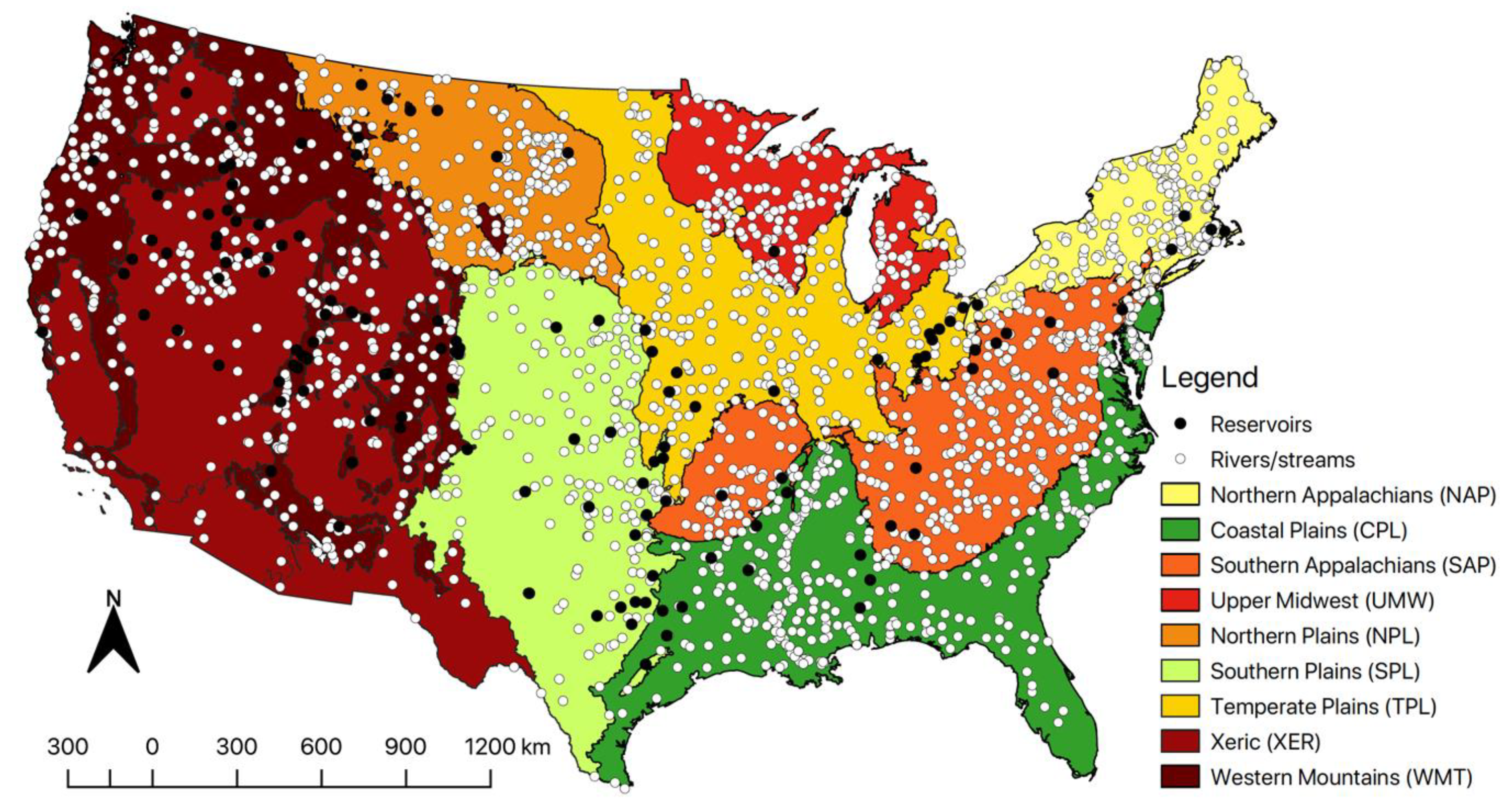
2.2.2. Ecoregions

Reservoirs and rivers were distributed across nine terrestrial ecoregions, a priori defined by Omernik [52] and Herlihy et al. [53]. Ecoregions are based on similar environmental characteristics (climate, vegetation, soil type and geology) and macroinvertebrate assemblages (Figure 1); Coastal Plains (CPL), Northern Appalachians (NAP), Northern Plains (NPL), Southern Appalachians (SAP), Southern Plains (SPL) Temperate Plains (TPL), Upper Midwest (UMW), Western Mountains (WMT) and Xeric (XER). This aggregation of ecoregion was adopted for both the NLA and NRSA surveys [54]. For each ecoregion, we also extracted land cover variables [54] (Table 1; spatial matrix) and variables related to human impacts (Table 1; human matrix).

2.2.3. Native Riverine Taxa Definition

The taxa pool observed in rivers and streams was used as a baseline to compare taxa richness before and after reservoir occupation (reference; native riverine taxa). We used only native riverine taxa and excluded all new taxa that would be encountered in a lake-like habitat (reservoir), since they would most likely not be present in a pre-reservoir occupation, river-like habitat. We considered using pairwise comparisons (impacted site paired with a single reference site) or reference sites found within a fixed radius or within the ecoregion. We decided to go with an ecoregion mean reference because there is neither literature to support the choice of a singular river when multiple rivers were surrounding a reservoir nor to support a fixed radius distance (25 km, 50 km). Comparing to a mean reference in each ecoregion, instead of a single river or stream close to the reservoir, ensures that we are measuring the impacts from a set of reference conditions and not a singular pristine, or impacted, river or stream. Moreover, as specified in Section 2.2.2, ecoregions were defined based on similar macroinvertebrate assemblages, which further reinforce the choice of this scale, at the ecological point of view, for our study.

2.2.4. PDFs Calculation

We calculated PDFs as the difference in richness between river (x) and reservoir richness (y), divided by the river richness (x). The PDF is a dimensionless proportion ranging between −1 and 1. At the United States scale ($\mathrm{P}\mathrm{D}{\mathrm{F}}_{\mathrm{u}\mathrm{s}\mathrm{a}}$), we compared the overall United States mean native riverine richness in rivers and streams (one observation of richness per river or stream averaged over the United States; ${\overline{x}}_{usa}$; n = 2062) to the overall United States mean richness in reservoirs (one observation of richness per reservoir averaged over the United States; ${\overline{y}}_{usa}$; n = 134) to obtain a United States-specific change in richness, as per Equation (1);

$$\mathrm{P}\mathrm{D}{\mathrm{F}}_{\mathrm{u}\mathrm{s}\mathrm{a}}=\frac{{\overline{x}}_{usa}- {\overline{y}}_{usa}}{{\overline{x}}_{usa}}$$

(1)

At the ecoregion scale ($\mathrm{P}\mathrm{D}{\mathrm{F}}_{\mathrm{e}\mathrm{c}\mathrm{o}}$), we compared ecoregion mean native riverine richness of all rivers and streams (one observation of richness per river or stream averaged over each ecoregion; ${\overline{x}}_{eco}$) to the ecoregion mean richness in reservoirs (one observation of richness per reservoir averaged over each ecoregion; ${\overline{y}}_{eco}$) to obtain an ecoregion-specific change in richness, as per Equation (2);

$$\mathrm{P}\mathrm{D}{\mathrm{F}}_{\mathrm{e}\mathrm{c}\mathrm{o}}=\frac{{\overline{x}}_{eco}- {\overline{y}}_{eco}}{{\overline{x}}_{eco}}$$

(2)

At the reservoir scale ($\mathrm{P}\mathrm{D}{\mathrm{F}}_{\mathrm{r}\mathrm{e}\mathrm{s}}$), we compared ecoregion mean native riverine richness of all rivers and streams (one observation of richness per river or stream averaged over each ecoregion; ${\overline{x}}_{eco}$) to the richness of a specific reservoir within the same ecoregion (one specific richness observation per reservoir, no averaging; $y_{res}$) to obtain a reservoir-specific change in richness, as per Equation (3);

$$\mathrm{P}\mathrm{D}{\mathrm{F}}_{\mathrm{r}\mathrm{e}\mathrm{s}}=\frac{{\overline{x}}_{eco}- y_{res}}{{\overline{x}}_{eco}}$$

(3)

2.3. Data Analysis and Empirical Modelling

2.3.1. Regionalization and ANOVA

Regionalization is a critical aspect in LCA [55,56]. It accounts for existing spatial variability to improve results’ representativeness and reduce spatial uncertainties [55]. CFs must be developed at an appropriate scale to capture the environmental impacts of a product, process or service, and inform decision makers. As a first step, we ran a one-way randomized-group analysis of variance (ANOVA) to determine whether PDF_eco differed across ecoregions (ecoregion scale) and thus test the relevance of this regionalization scale. We assessed the significance of regionalization at the ecoregion scale and identified which ecoregions were significantly different from each other based on the standardized mean difference and its confidence interval (CI). All statistical analyses were made using R version 3.0.2 [57]. We conducted the ANOVA with the ind.oneway.second function in the rpsychi R package version 0.8 [58].

2.3.2. Variation Partitioning to Explain the Variation Observed in Our PDF_res

As a second step, we were interested in understanding which variables explained the variation observed in PDF_res at the reservoir scale in the United States. To do so, we used variation partitioning [59], a statistical analysis that describes how a set of explanatory matrices explains the shared variation observed in a response variable (PDF). We built four explanatory matrices (spatial, physical, chemical and human matrices) based on the available descriptive variables from the NLA and NRSA datasets and selected a set of variables potentially influencing macroinvertebrate richness based on expert judgment. The spatial matrix included variables describing the location of the reservoirs; latitude, longitude, ecoregion, temperature, precipitation and types of land covers (forested, cultivated pastures, wetlands, grasslands and shrubs, developed and water or barren). The physical matrix included variables describing the reservoir; reservoir area, elevation, shallow water and riparian vegetation. The chemical matrix included variables that describe the biochemical state of the reservoir; trophic state, Secchi depth, dissolved organic carbon (DOC), total phosphorus level (TPL), water color, conductivity, total nitrogen level (TNL), pH, methylmercury and chlorophyll-α (Chl-α). The human matrix included variables describing the human activity, impact or influence around the reservoir shoreline; influence of buildings, commercial activities, crops, docks, landfills, lawns, parks, pastures, powerlines, roads, walls and others. See Table 1 for a complete description of the variables included in each matrix. To achieve the most parsimonious analysis, we performed a stepwise selection procedure on each explanatory matrix to identify which variable, or combination of variables, best-explained the variation in PDF_res (variables in bold; Table 1). Variable selection was performed with the function ordiR2step and variation partitioning was conducted with the varpart function in the vegan R package version 2.5-2 [60].

2.3.3. Empirical Modelling

As a third step, we used a multiple linear regression (lm function in the stat R package version 3.4.2; [57]) to develop an empirical model to be used by LCA modellers and practitioners. This empirical model can be used to assess PDF_res from known values of explanatory variables (related to the reservoir, not the rivers and streams) when we do not have information about empirical change in macroinvertebrate richness in impacted and/or reference sites, within a specific frame of application and range of environmental variables (also called interpolation). We used the variables identified by the variation partitioning analysis as the most influential variables to explain the variation in PDF_res. We checked whether assumptions associated with multiple linear regression were violated (the residuals are independent, normal, have a mean of 0 and are homoscedastic; Figure A1 and Figure A2), we deleted a few outliers, and performed a model selection procedure. We applied a manual backward selection procedure, used the recommended information theoretic approach based on the Akaike information criterion (AIC; [61]) and the Bayesian information criterion (BIC; [62]) to compare the seven candidate models, and selected the model with the highest support (

Table 2. Summary of statistical candidate models (Akaike information criterion; ΔAIC, and Bayesian information criterion; BIC), where PDF stands for Potentially Disappeared Fraction of species, ELE for elevation, AREA for surface area, T.S. for trophic state, PH for pH level, LAWN for influence of lawns and ROAD for influence of roads. For each candidate model, the estimate for the intercept is labelled b_int and all other bs (b_ELE, b_AREA, b_T.S., b_PH, b_LAWN, and b_ROAD) estimate for the slope of their respective variable. See Table 1 for full description of the variables used. ^§ Marginally significant.

Models	Non-Significant Variables	ΔAIC	BIC
(A) PDF~bint + bELE*sqrt(ELE) + bAREA*log10(AREA) + bT.S.*T.S. + bPH*PH + bLAWN*log10(LAWN) + bROAD*log10(ROAD)	PH §, LAWN and ROAD	2	27
(B) PDF~bint + bELE*sqrt(ELE) + bAREA*log10(AREA) + bT.S.*T.S. + bPH*PH + bLAWN*log10(LAWN)	PH § and LAWN	1	24
(C) PDF~bint + bELE*sqrt(ELE) + bAREA*log10(AREA) + bT.S.*T.S. + bPH*PH	PH §	0	20
(D) PDF~bint + bELE*sqrt(ELE) + bAREA*log10(AREA) + bT.S.*T.S.	None	2	20
(E) PDF~bint + bELE*sqrt(ELE) + bAREA*log10(AREA)	None	8	23
(F) PDF~bint + bELE*sqrt(ELE)	None	19	32
(G) PDF~bint	-	52	63

). For each explanatory variable selected in the final model, we extracted estimates and standard error (SE), where the estimates represent the direction and magnitude of PDF_res.

3. Results

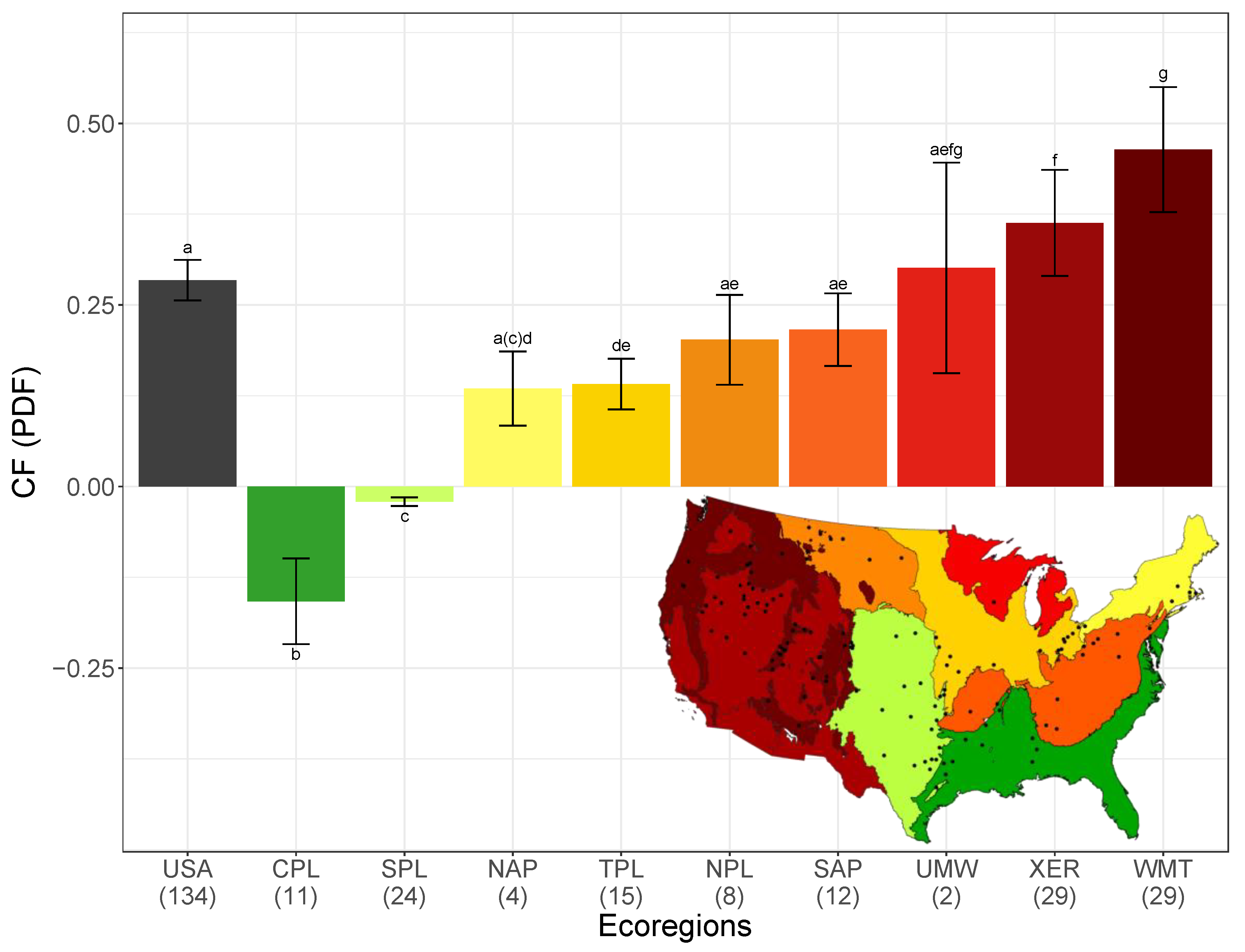
3.1. PDF_usa and Variation in PDF_eco across Ecoregions

A total of 973 native riverine macroinvertebrate taxa were inventoried throughout the United States. The mean native riverine richness per ecoregion varied from 26.1 ± 13.1 to 46.0 ± 13.8 (mean ± standard deviation [SD];

Table 3. Table showing the mean native riverine richness for each ecoregion (± standard deviation; SD), sample number from which mean native riverine richness was computed (n.riv), mean impacted reservoir richness for each ecoregion (±SD), Potentially Disappeared Fraction of Species (PDF ± SD and ±95% confidence interval [CI]) values and the sample number (n.res) from which mean reservoir richness and PDF was calculated is also shown for the United States and the nine ecoregions. A positive PDF represents a loss of taxa, whereas a negative PDF represents a gain of taxa.

Ecoregion or Country	Mean Nat. Riv. Richness	±SD	n.riv	Mean Imp. Res. Richness	±SD	PDF · m2·yr/m2·yr	±SD	±95% CI	n.res
USA	35.9	15.5	2062	25.7	10.4	0.284	0.168	0.028	134
CPL	28.4	16.6	327	32.9	7.9	−0.158	−0.100	−0.059	11
SPL	26.1	13.1	176	26.7	11.8	−0.021	−0.014	−0.006	24
NAP	46.0	13.8	225	39.8	9.4	0.135	0.052	0.051	4
TPL	32.0	12.9	209	27.5	7.7	0.141	0.069	0.035	15
NPL	29.4	10.1	179	23.5	6.6	0.202	0.090	0.062	8
SAP	45.8	15.1	344	35.9	8.8	0.216	0.089	0.050	12
UMW	39.3	12.7	167	27.5	3.5	0.301	0.105	0.145	2
XER	31.0	11.6	213	19.7	7.9	0.363	0.199	0.073	29
WMT	39.8	12.0	222	21.3	8.6	0.464	0.235	0.086	29

and

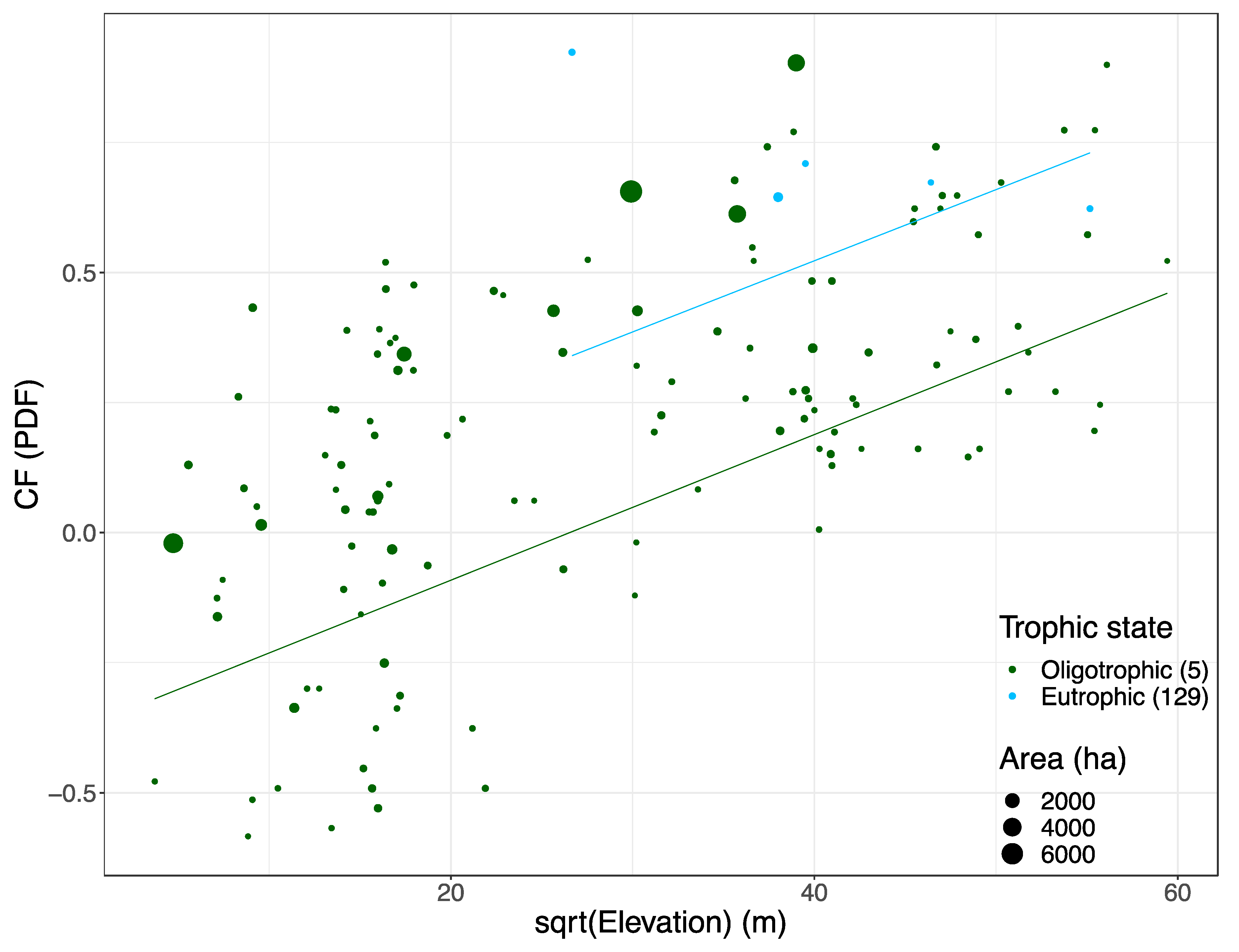
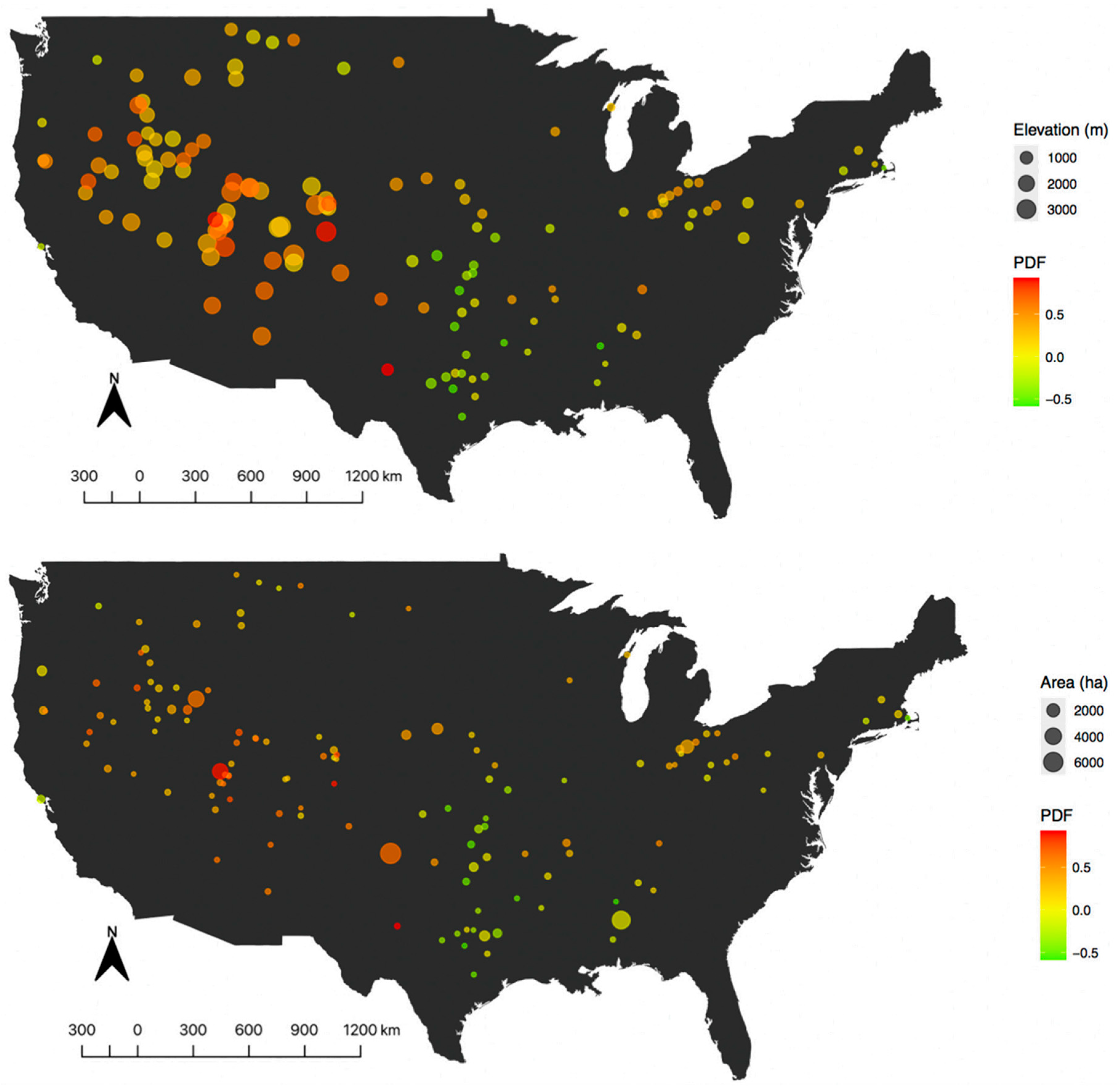
Table A1. Raw data table for our study of reservoir richness in the United States including variables such as the unique identifier (UID) for each reservoir, latitude (LAT), longitude (LON), ecoregion (ECO), elevation (ELE; in meters), area (AREA; in hectares), trophic state (TS), number of river and stream samples in the ecoregion (N.REF), mean native riverine richness per ecoregion (MEAN.REF.S), standard deviation of the mean native riverine richness per ecoregion (SD.REF.S), number of reservoir samples (N.IMP; at the reservoir level hence always one), reservoir richness (IMP.S; specific to each reservoir, not a mean), standard deviation of the reservoir richness (SD.IMP.S; one reservoir, thus standard deviation always zero), Potentially Disappeared Fraction of species (PDF), standard deviation associated to the Potentially Disappeared Fraction of species (SD.PDF), lower confidence interval (LOW.CI) and higher confidence interval (UP.CI).

UID	LAT	LON	ECO	ELE	AREA	TS	N.REF	MEAN.REF.S	SD.REF.S	N.IMP	IMP.S	SD.IMP.S	PDF	SD.PDF	LOW.CI	UP.CI
6243	38.507965	−94.673265	TPL	295.8	110.0	EUT	209	32.0	12.9	1	42	0	−0.314	0.126	−0.562	−0.066
6252	40.111767	−75.861530	SAP	186.7	63.2	EUT	344	45.8	15.1	1	35	0	0.236	0.078	0.083	0.388
6267	31.621546	−88.353739	CPL	50.8	32.6	EUT	327	28.4	16.6	1	32	0	−0.126	0.074	−0.271	0.019
6270	35.174388	−99.077489	SPL	499.9	141.5	EUT	176	26.1	13.1	1	14	0	0.465	0.233	0.007	0.922
6281	35.285013	−112.154163	WMT	2072.1	24.8	EUT	222	39.8	12.0	1	15	0	0.623	0.188	0.254	0.992
6319	36.831633	−104.226303	WMT	2066.2	44.2	EUT	222	39.8	12.0	1	16	0	0.598	0.181	0.243	0.952
6342	39.994962	−105.112227	SPL	1620.9	18.2	EUT	176	26.1	13.1	1	26	0	0.006	0.003	0.000	0.011
6404	39.638354	−95.456811	TPL	321.7	26.9	EUT	209	32.0	12.9	1	22	0	0.312	0.126	0.066	0.558
6437	39.000154	−95.779648	TPL	350.6	101.9	EUT	209	32.0	12.9	1	34	0	−0.064	0.026	−0.114	−0.013
6451	40.161787	−79.052384	SAP	551.9	18.2	EUT	344	45.8	15.1	1	43	0	0.061	0.020	0.022	0.101
6481	39.484355	−118.723571	XER	1202.0	164.1	EUT	213	31.0	11.6	1	19	0	0.387	0.144	0.104	0.670
6482	41.928985	−119.179002	XER	1678.2	100.3	EUT	213	31.0	11.6	1	16	0	0.484	0.181	0.129	0.838
6501	35.980828	−108.931643	WMT	2290.2	15.4	EUT	222	39.8	12.0	1	14	0	0.648	0.196	0.264	1.032
6525	35.992932	−96.873677	SPL	255.6	177.7	EUT	176	26.1	13.1	1	40	0	−0.530	0.266	−1.051	−0.009
6550	34.953616	−96.718159	SPL	281.1	533.1	EUT	176	26.1	13.1	1	27	0	−0.033	0.016	−0.065	−0.001
6556	35.412203	−95.929276	SPL	201.3	204.3	EUT	176	26.1	13.1	1	25	0	0.044	0.022	0.001	0.087
6570	37.655565	−98.260986	SPL	479.3	56.8	EUT	176	26.1	13.1	1	39	0	−0.492	0.247	−0.975	−0.008
6575	40.723819	−109.183908	XER	2184.0	43.3	EUT	213	31.0	11.6	1	21	0	0.322	0.120	0.086	0.558
6586	31.787274	−96.064492	CPL	91.4	852.5	EUT	327	28.4	16.6	1	28	0	0.015	0.009	−0.002	0.031
6599	46.543922	−104.028258	NPL	907.4	3.8	EUT	179	29.4	10.1	1	33	0	−0.121	0.042	−0.203	−0.040
6606	37.390887	−99.784838	SPL	685.8	127.3	EUT	176	26.1	13.1	1	28	0	−0.071	0.036	−0.141	−0.001
6617	41.757410	−115.722027	XER	2089.2	23.6	EUT	213	31.0	11.6	1	26	0	0.161	0.060	0.043	0.279
6618	41.198060	−115.892296	XER	1814.2	5.0	EUT	213	31.0	11.6	1	26	0	0.161	0.060	0.043	0.279
6622	31.889172	−97.702492	SPL	290.0	20.7	EUT	176	26.1	13.1	1	35	0	−0.339	0.170	−0.672	−0.005
6668	36.823001	−96.047588	SPL	230.6	103.5	EUT	176	26.1	13.1	1	38	0	−0.453	0.228	−0.899	−0.007
6695	36.705443	−96.419109	TPL	266.8	325.4	EUT	209	32.0	12.9	1	40	0	−0.251	0.101	−0.450	−0.053
6719	38.398162	−115.117053	XER	1574.3	72.3	EUT	213	31.0	11.6	1	23	0	0.258	0.096	0.069	0.446
6731	41.701690	−113.959671	XER	1622.6	10.3	EUT	213	31.0	11.6	1	26	0	0.161	0.060	0.043	0.279
6735	32.944430	−96.453752	SPL	146.0	13.8	EUT	176	26.1	13.1	1	34	0	−0.300	0.151	−0.596	−0.005
6742	47.761716	−108.432829	NPL	912.2	4.3	EUT	179	29.4	10.1	1	30	0	−0.019	0.007	−0.032	−0.006
6753	39.931042	−104.973296	SPL	1600.5	9.2	EUT	176	26.1	13.1	1	20	0	0.235	0.118	0.004	0.466
6762	33.516175	−94.125132	CPL	82.4	17.1	EUT	327	28.4	16.6	1	43	0	−0.513	0.301	−1.103	0.076
6774	46.826042	−100.634208	NPL	523.4	3.9	EUT	179	29.4	10.1	1	16	0	0.456	0.157	0.149	0.764
6795	38.997241	−108.051180	WMT	3070.9	15.0	EUT	222	39.8	12.0	1	32	0	0.195	0.059	0.080	0.311
6796	37.193346	−95.988976	SPL	252.1	13.5	EUT	176	26.1	13.1	1	36	0	−0.377	0.189	−0.748	−0.006
6806	38.491412	−79.314781	SAP	604.1	3.8	EUT	344	45.8	15.1	1	43	0	0.061	0.020	0.022	0.101
6823	43.165878	−115.652476	XER	997.2	163.9	EUT	213	31.0	11.6	1	24	0	0.225	0.084	0.060	0.390
6868	38.235087	−112.463009	WMT	2680.7	9.6	EUT	222	39.8	12.0	1	26	0	0.346	0.105	0.141	0.551
6869	38.847537	−111.961390	XER	1589.5	93.2	EUT	213	31.0	11.6	1	16	0	0.484	0.181	0.129	0.838
6874	39.036703	−107.911131	WMT	3105.2	5.7	EUT	222	39.8	12.0	1	30	0	0.246	0.074	0.100	0.391
6875	40.944919	−106.011968	XER	2410.4	17.4	EUT	213	31.0	11.6	1	26	0	0.161	0.060	0.043	0.279
6923	40.039991	−81.013888	SAP	322.7	43.0	EUT	344	45.8	15.1	1	24	0	0.476	0.157	0.168	0.784
6940	44.329096	−116.184107	WMT	1507.0	71.6	EUT	222	39.8	12.0	1	29	0	0.271	0.082	0.110	0.431
6944	39.169507	−111.450721	WMT	2837.7	18.8	EUT	222	39.8	12.0	1	29	0	0.271	0.082	0.110	0.431
6959	44.964115	−116.463019	WMT	1453.0	211.4	EUT	222	39.8	12.0	1	32	0	0.195	0.059	0.080	0.311
6966	39.142411	−111.452546	WMT	2889.5	27.9	EUT	222	39.8	12.0	1	9	0	0.774	0.234	0.315	1.232
6970	44.796705	−116.732688	WMT	2154.4	12.4	OLI	222	39.8	12.0	1	13	0	0.673	0.204	0.274	1.072
6971	43.191413	−116.959804	XER	1399.8	73.0	EUT	213	31.0	11.6	1	8	0	0.742	0.277	0.199	1.285
6976	38.791149	−105.106361	WMT	3147.0	10.2	EUT	222	39.8	12.0	1	4	0	0.899	0.272	0.366	1.433
7020	38.078326	−122.743359	XER	51.1	335.3	EUT	213	31.0	11.6	1	36	0	−0.162	0.061	−0.281	−0.043
7057	39.204737	−111.668912	WMT	1789.8	24.8	EUT	222	39.8	12.0	1	30	0	0.246	0.074	0.100	0.391
7097	38.788187	−111.774878	WMT	2203.2	6.7	EUT	222	39.8	12.0	1	15	0	0.623	0.188	0.254	0.992
7100	43.965218	−122.683968	WMT	255.3	709.5	EUT	222	39.8	12.0	1	37	0	0.070	0.021	0.028	0.111
7105	41.110516	−82.083872	NAP	258.0	21.0	EUT	225	46.0	13.8	1	28	0	0.391	0.118	0.160	0.622
7108	30.963438	−95.903504	CPL	86.9	27.3	EUT	327	28.4	16.6	1	27	0	0.050	0.029	−0.007	0.107
7109	32.072696	−97.129773	SPL	186.9	12.6	EUT	176	26.1	13.1	1	24	0	0.082	0.041	0.001	0.163
7136	41.633291	−118.389357	XER	1311.6	15.4	EUT	213	31.0	11.6	1	23	0	0.258	0.096	0.069	0.446
7205	32.240254	−101.313303	SPL	711.1	56.8	OLI	176	26.1	13.1	1	2	0	0.924	0.464	0.015	1.832
7207	42.157825	−122.607634	WMT	684.2	256.5	EUT	222	39.8	12.0	1	26	0	0.346	0.105	0.141	0.551
7226	42.130013	−122.478277	WMT	1344.3	4.4	EUT	222	39.8	12.0	1	19	0	0.522	0.158	0.213	0.832
7228	34.227816	−86.843449	SAP	247.0	73.0	EUT	344	45.8	15.1	1	44	0	0.039	0.013	0.014	0.065
7229	40.631585	−120.002870	XER	1329.5	37.1	EUT	213	31.0	11.6	1	20	0	0.354	0.132	0.095	0.614
7232	40.703407	−83.378745	TPL	269.7	102.7	EUT	209	32.0	12.9	1	17	0	0.468	0.189	0.099	0.838
7276	41.168583	−119.817451	XER	1560.8	28.9	OLI	213	31.0	11.6	1	9	0	0.710	0.265	0.190	1.229
7294	39.056042	−82.690673	SAP	211.5	65.1	EUT	344	45.8	15.1	1	47	0	−0.026	0.009	−0.043	−0.009
7304	31.587497	−98.622503	SPL	448.8	27.8	EUT	176	26.1	13.1	1	36	0	−0.377	0.189	−0.748	−0.006
7306	39.241149	−117.165818	XER	2255.5	5.8	EUT	213	31.0	11.6	1	19	0	0.387	0.144	0.104	0.670
7325	40.337080	−105.126694	SPL	1562.4	189.8	EUT	176	26.1	13.1	1	19	0	0.273	0.137	0.004	0.542
7368	32.515869	−87.861085	CPL	22.3	4731.5	EUT	327	28.4	16.6	1	29	0	−0.021	0.012	−0.044	0.003
7369	41.035420	−96.837727	TPL	391.7	29.2	EUT	209	32.0	12.9	1	26	0	0.187	0.075	0.039	0.334
7375	33.364862	−88.166880	CPL	78.1	5.6	EUT	327	28.4	16.6	1	45	0	−0.584	0.342	−1.254	0.086
7392	34.534351	−92.268826	CPL	74.1	105.8	EUT	327	28.4	16.6	1	26	0	0.085	0.050	−0.013	0.182
7402	34.284778	−97.170972	SPL	245.4	160.7	EUT	176	26.1	13.1	1	39	0	−0.492	0.247	−0.975	−0.008
7405	40.328099	−96.532001	TPL	425.9	32.1	EUT	209	32.0	12.9	1	25	0	0.218	0.088	0.046	0.390
7409	33.075563	−92.660596	CPL	55.4	7.3	EUT	327	28.4	16.6	1	31	0	−0.091	0.053	−0.196	0.013
7459	33.882010	−85.931618	SAP	171.0	18.1	EUT	344	45.8	15.1	1	39	0	0.148	0.049	0.052	0.244
7471	46.040623	−110.692175	NPL	1556.2	96.7	EUT	179	29.4	10.1	1	23	0	0.219	0.075	0.071	0.366
7472	46.624624	−110.738336	NPL	1672.9	150.7	EUT	179	29.4	10.1	1	25	0	0.151	0.052	0.049	0.252
7533	43.078399	−112.693659	XER	1338.8	21.3	EUT	213	31.0	11.6	1	14	0	0.548	0.205	0.147	0.949
7572	40.372482	−84.340110	TPL	291.8	327.1	EUT	209	32.0	12.9	1	22	0	0.312	0.126	0.066	0.558
7579	39.608156	−84.971507	TPL	254.8	72.8	EUT	209	32.0	12.9	1	21	0	0.343	0.138	0.072	0.614
7643	39.706824	−111.293369	WMT	2569.0	31.5	EUT	222	39.8	12.0	1	29	0	0.271	0.082	0.110	0.431
7652	40.176639	−84.265220	TPL	275.4	15.3	EUT	209	32.0	12.9	1	29	0	0.093	0.037	0.020	0.166
7684	37.673281	−107.112778	WMT	3530.5	2.1	EUT	222	39.8	12.0	1	19	0	0.522	0.158	0.213	0.832
7686	37.316232	−107.112994	WMT	2348.4	35.2	EUT	222	39.8	12.0	1	34	0	0.145	0.044	0.059	0.231
7698	41.152339	−110.824953	XER	2180.1	90.9	EUT	213	31.0	11.6	1	8	0	0.742	0.277	0.199	1.285
7713	46.118216	−113.374640	WMT	1847.6	152.3	EUT	222	39.8	12.0	1	26	0	0.346	0.105	0.141	0.551
7800	41.677573	−73.144698	NAP	198.8	56.2	EUT	225	46.0	13.8	1	51	0	−0.109	0.033	−0.174	−0.045
7810	43.413998	−119.410472	XER	1268.6	107.8	EUT	213	31.0	11.6	1	10	0	0.677	0.253	0.181	1.173
7812	35.562459	−93.637568	SAP	203.7	44.7	EUT	344	45.8	15.1	1	28	0	0.389	0.128	0.137	0.640
8016	33.829304	−109.090421	WMT	2403.4	48.4	EUT	222	39.8	12.0	1	17	0	0.573	0.173	0.233	0.912
8121	36.067203	−91.142428	SAP	82.7	222.6	EUT	344	45.8	15.1	1	26	0	0.432	0.143	0.153	0.712
8144	35.583189	−90.962941	CPL	69.0	95.9	EUT	327	28.4	16.6	1	21	0	0.261	0.153	−0.038	0.560
8151	41.088461	−82.729015	TPL	249.8	80.7	EUT	209	32.0	12.9	1	26	0	0.187	0.075	0.039	0.334
8184	40.055586	−105.747080	WMT	3029.0	51.0	EUT	222	39.8	12.0	1	17	0	0.573	0.173	0.233	0.912
8207	39.653475	−82.473781	SAP	240.2	47.7	EUT	344	45.8	15.1	1	44	0	0.039	0.013	0.014	0.065
8250	48.380621	−110.985266	NPL	913.5	9.5	EUT	179	29.4	10.1	1	20	0	0.321	0.110	0.105	0.537
8256	39.775971	−81.522472	SAP	241.9	24.2	EUT	344	45.8	15.1	1	36	0	0.214	0.071	0.076	0.352
8278	48.026569	−109.623760	NPL	1128.8	9.8	EUT	179	29.4	10.1	1	27	0	0.083	0.028	0.027	0.138
8325	37.416782	−108.405651	WMT	2213.0	65.4	EUT	222	39.8	12.0	1	14	0	0.648	0.196	0.264	1.032
8342	32.056309	−96.731783	SPL	162.6	5.5	EUT	176	26.1	13.1	1	34	0	−0.300	0.151	−0.596	−0.005
8360	40.674602	−110.970699	WMT	3043.5	39.4	OLI	222	39.8	12.0	1	15	0	0.623	0.188	0.254	0.992
8395	40.889268	−109.846108	WMT	2622.7	32.5	EUT	222	39.8	12.0	1	24	0	0.397	0.120	0.161	0.632
8409	39.720767	−86.720223	TPL	255.2	124.2	EUT	209	32.0	12.9	1	30	0	0.062	0.025	0.013	0.110
8413	31.910344	−95.301856	CPL	129.5	481.4	EUT	327	28.4	16.6	1	38	0	−0.337	0.198	−0.725	0.050
8414	40.121695	−104.945911	SPL	1509.8	24.7	EUT	176	26.1	13.1	1	6	0	0.771	0.387	0.012	1.529
8416	38.939348	−91.282857	TPL	226.5	4.3	EUT	209	32.0	12.9	1	37	0	−0.157	0.063	−0.282	−0.033
8427	44.698479	−87.499926	UMW	179.8	35.5	EUT	167	39.3	12.7	1	30	0	0.237	0.077	0.087	0.388
8435	47.876688	−107.125232	NPL	758.1	13.8	EUT	179	29.4	10.1	1	14	0	0.524	0.180	0.171	0.878
8437	42.646907	−72.218497	NAP	195.1	138.4	EUT	225	46.0	13.8	1	40	0	0.130	0.039	0.053	0.206
8443	41.812487	−70.638227	CPL	13.7	10.8	EUT	327	28.4	16.6	1	42	0	−0.478	0.280	−1.027	0.071
8480	30.006973	−96.709810	SPL	109.8	21.4	EUT	176	26.1	13.1	1	39	0	−0.492	0.247	−0.975	−0.008
8487	39.661693	−84.646207	TPL	287.3	7.1	EUT	209	32.0	12.9	1	20	0	0.374	0.151	0.079	0.670
8494	41.989559	−71.205066	NAP	30.9	202.4	EUT	225	46.0	13.8	1	40	0	0.130	0.039	0.053	0.206
8495	46.941268	−119.278530	XER	263.5	53.1	EUT	213	31.0	11.6	1	34	0	−0.097	0.036	−0.169	−0.026
8504	38.070619	−111.375127	WMT	3074.1	11.2	EUT	222	39.8	12.0	1	9	0	0.774	0.234	0.315	1.232
8614	36.044443	−85.586295	SAP	269.0	30.2	EUT	344	45.8	15.1	1	22	0	0.520	0.171	0.184	0.856
8635	40.495536	−83.899880	TPL	303.7	2018.9	EUT	209	32.0	12.9	1	21	0	0.343	0.138	0.072	0.614
8765	37.595562	−112.254669	WMT	2389.9	70.2	EUT	222	39.8	12.0	1	25	0	0.371	0.112	0.151	0.592
8766	40.863781	−109.811815	WMT	2528.1	18.1	EUT	222	39.8	12.0	1	13	0	0.673	0.204	0.274	1.072
8777	39.360351	−111.963708	XER	1521.4	3220.7	EUT	213	31.0	11.6	1	3	0	0.903	0.337	0.242	1.565
8811	31.331826	−97.268438	SPL	180.5	14.8	EUT	176	26.1	13.1	1	41	0	−0.568	0.285	−1.127	−0.009
1000019	43.460190	−116.141301	XER	973.1	33.4	EUT	213	31.0	11.6	1	25	0	0.193	0.072	0.052	0.334
1000025	43.198407	−114.599726	XER	1678.7	44.6	EUT	213	31.0	11.6	1	27	0	0.129	0.048	0.034	0.223
1000029	42.677045	−113.407296	XER	1278.7	3395.5	EUT	213	31.0	11.6	1	12	0	0.613	0.229	0.164	1.061
1000030	42.206372	−114.878852	XER	1593.0	393.0	EUT	213	31.0	11.6	1	20	0	0.354	0.132	0.095	0.614
1000068	46.206071	−116.834367	XER	1034.1	38.1	EUT	213	31.0	11.6	1	22	0	0.290	0.108	0.078	0.502
1000073	35.582330	−101.717139	SPL	894.9	6559.4	EUT	176	26.1	13.1	1	9	0	0.656	0.329	0.011	1.301
1000084	41.037407	−100.775775	SPL	916.0	641.0	EUT	176	26.1	13.1	1	15	0	0.426	0.214	0.007	0.846
1000086	41.321987	−98.900675	SPL	657.7	1117.9	EUT	176	26.1	13.1	1	15	0	0.426	0.214	0.007	0.846
1000122	42.264258	−116.310496	XER	1690.0	35.5	EUT	213	31.0	11.6	1	25	0	0.193	0.072	0.052	0.334
1000126	42.531475	−116.364513	XER	1773.6	29.4	EUT	213	31.0	11.6	1	23	0	0.258	0.096	0.069	0.446
1000137	42.187306	−113.924080	XER	1444.7	407.4	OLI	213	31.0	11.6	1	11	0	0.645	0.241	0.173	1.117
1000223	43.537123	−90.959353	UMW	277.4	14.8	EUT	167	39.3	12.7	1	25	0	0.364	0.118	0.133	0.595

). The mean reservoir richness per ecoregion varied from 19.7 ± 7.9 to 39.8 ± 9.4 (mean ± SD; Table 3). Our empirically derived PDF_usa and PDF_eco showed a loss in macroinvertebrate richness due to reservoir occupation in the United States and this loss followed a longitudinal gradient associated with the ecoregions (Figure 2). At the United States scale, 28% of macroinvertebrate taxa disappeared in response to river impoundment (PDF_usa = 0.284 ± 0.168 [mean ± SD]; Table 3 and Figure 2). At the ecoregion scale, seven out of nine ecoregions (78%) showed a statistically significant loss of macroinvertebrate taxa, with PDF_eco varying from 0.135 ± 0.052 to 0.464 ± 0.235. Two ecoregions (CPL and SPL), showed a significant increase in macroinvertebrate taxa (PDF_CPL = −0.158 ± 0.100 and PDF_SPL = −0.021 ± 0.014; Table 3 and Figure 2). PDF_CPL, PDF_SPL, PDF_XER and PDF_WMT significantly differed from most ecoregions, whereas PDF_NAP, PDF_TPL, PDF_NPL, PDF_SAP and PDF_UMW, showed much less significant differences (Figure 2). Those PDF_eco were mostly all characterized by smaller sample sizes (respectively, n = 4, 15, 8, 12 or 2). Results from the ANOVA suggest a longitudinal gradient of impact, where PDF_eco are higher in the western part of the country and lower in the eastern part of the country (Figure 2). At the reservoir scale, PDF_res varied from −0.584 ± 0.342 (observation ± pooled SD) to 0.924 ± 0.464, and 74% of the reservoirs showed a significant loss of macroinvertebrate taxa (Table A1).

3.2. Variables Explaining the Variation in PDF_res

At the reservoir scale, the four matrices (spatial, physical, chemical, and human) explained approximately 51% of the total variation in PDF_res (variation partitioning; Figure 3;

Table A2. Variation partitioning fractions (percentages) explained. [a] to [d] represent the fractions of variation explained uniquely by each of the four matrices, [a] being the spatial matrix, [b] the physical matrix, [c] the chemical matrix and [d] the human matrix. [e] to [j] are the joint fractions between two matrices ([e] is spatial and physical, [f] is physical and chemical, [g] is spatial and chemical, [h] is spatial and human, [i] is physical and human, [j] is chemical and human) and [k] to [n] the joint fractions between three matrices ([k] is spatial, physical and human, [l] is spatial, physical and chemical, [m] is physical, chemical and human, and [n] is spatial, chemical and human). Finally, [o] is the joint fraction between all four matrices.

%	[a]	[b]	[c]	[d]	[e]	[f]	[g]	[h]	[i]	[j]	[k]	[l]	[m]	[n]	[o]	Value
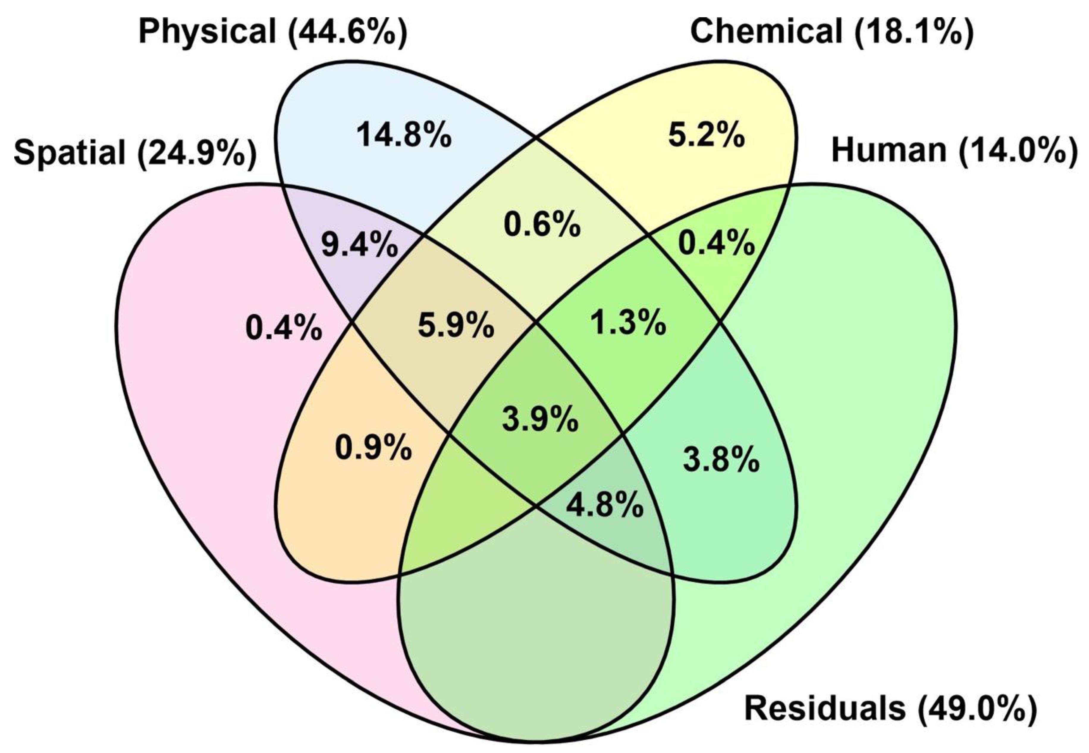
51	0.2	14.8	5.2	0.0	9.4	0.6	0.9	−0.2	3.8	0.4	4.8	5.9	1.3	−0.1	3.9	51.0
45	0.2	14.8			9.4	0.6	0.9	−0.2	3.8		4.8	5.9	1.3	−0.1	3.9	45.4
25	0.2				9.4		0.9	−0.2			4.8	5.9		−0.1	3.9	24.9
24					9.4						4.8	5.9			3.9	24.1
11							0.9					5.9		−0.1	3.9	10.7
8								−0.2			4.8			−0.1	3.9	8.4
45		14.8			9.4	0.6			3.8		4.8	5.9	1.3		3.9	44.6
15		14.8														14.8
18			5.2			0.6	0.9			0.4		5.9	1.3	−0.1	3.9	18.1
14				0.0				−0.2	3.8	0.4	4.8		1.3	−0.1	3.9	14.0

). Approximately 46% of the variation was explained by the combined effects of the spatial (ecoregion) and physical (elevation and surface area) matrices. Spatial matrix (ecoregion) explained 25% of the variation, over which 24% of this variation was shared with the physical matrix (elevation and surface area), 11% was shared with the chemical matrix (pH and trophic state), and 8% was shared with the human matrix (presence of lawn and road adjacent to the reservoir shoreline; Figure 3). The physical matrix explained 45% of the variation. Elevation and surface area alone (variation not shared with the other matrices) explained 15% of the variation. The chemical and human matrices explained, respectively, 18% and 14% of the variation.

3.3. PDF_res Empirical Model

According to the empirical model (Equations (4) and (5); Figure 4), almost 50% of the observed variation in PDF_res (partial R²_adj = 0.49; p < 0.001; n = 134) was explained by elevation (35%), trophic state (either oligotrophic or eutrophic; 4%), and reservoir surface area (10%). No more than 50% of the variation explained is acceptable in ecology disciplines, since there is substantial environmental variation that cannot be accounted for, unless specifically sampled for. PDF_res was positively related to reservoir elevation, where higher elevation was associated to higher PDF_res (Figure 4). PDF_res was negatively related to eutrophication status. Oligotrophic reservoirs (<10 μg/L total phosphorus) had higher PDF_res than eutrophic reservoirs (>10 μg/L total phosphorus). As for reservoir surface area, there was a positive relationship between reservoir surface area and PDF_res, where bigger reservoirs had a higher PDF_res than smaller ones (Figure 4). To summarize, large oligotrophic reservoirs located at higher elevation were most likely to have higher macroinvertebrate PDF_res.

$${\mathrm{PDF}}_{\mathrm{res}\left[\mathrm{OLIGOTROPHIC}\right]}= -0.129\left(\pm 0.109\right)+ 0.013\left(\pm 0.002\right)·\mathrm{sqrt}\left(\mathrm{ELE}\right)+0.170\left(\pm 0.043\right)·{\log }_{10}\left(\mathrm{AREA}\right)$$

(4)

Values in parentheses are SE of the estimate.

$${\mathrm{PDF}}_{\mathrm{res}\left[\mathrm{EUTROPHIC}\right]}= -0.454\left(\pm 0.102\right)+ 0.013\left(\pm 0.002\right)·\mathrm{sqrt}\left(\mathrm{ELE}\right)+0.170\left(\pm 0.043\right)·{\log }_{10}\left(\mathrm{AREA}\right)$$

(5)

4. Discussion

From the examination of 134 reservoirs of varied usages (flood control [n = 6], hydropower [n = 2], recreational [n = 23], soil erosion prevention [n = 5], transport [n = 2], water supply [n = 49] and unknown [n = 47]) and 2062 rivers and streams across the continental United States, our results showed a general loss of approximately 28% (PDF_usa) of macroinvertebrate taxa following reservoir occupation at the scale of the United States. PDF_eco also varied across ecoregions. Almost 25% of the total variation observed in PDF_res was explained by the nine ecoregions, pressing the need for regionalized CFs. We provided evidence that the empirical PDFs for macroinvertebrates were consistent and uniform across the three spatial scales (macroinvertebrate taxa loss at the scale of the country; PDF_usa, the majority of ecoregions; PDF_eco, and most reservoirs; PDF_res). Overall, the empirical PDFs derived in this study can be used as CFs in the LCA framework to evaluate the potential impact of reservoir occupation on the ecosystem quality AoP for a specific reservoir (PDF_res), within a given ecoregion (PDF_eco) or over the United States (PDF_usa). Potential impact scores expressed in PDF·m²·yr can be calculated multiplying PDF by the area-time occupied by the reservoir for a given product or service. We also provided a simple empirical model based on three explanatory variables (elevation, trophic state and reservoir surface area) that explained 49% of the variation in macroinvertebrate PDF_res. Reservoirs at higher elevation, with lower levels of eutrophication and bigger surface area had higher PDF_res. This empirical model could be used by LCA practitioners to interpolate CFs based on few explanatory variables. However, we did not test the transferability of our model to other countries, or to reservoirs outside of the ranges of application of this model (elevation between 13 and 3531 meters [m] and area between 2 and 6560 hectares [ha] for eutrophic reservoirs, and elevation between 711 and 3044 m and area between 12 and 408 ha for oligotrophic reservoirs; specific regression lines in Figure 4).

4.1. United States Taxa Loss and Regionalization

At the scale of the United States, 28% of macroinvertebrate taxa disappeared following reservoir occupation. This result suggests that reservoir occupation does affect the rate of change in macroinvertebrate richness, and this is consistent with the literature estimates of the impacts of hydropower on macroinvertebrate richness across the world [17,18,19,20,21,22,23,24,25,26]. Presently, there is still no macroinvertebrate CF (PDF) available to assess potential impacts of reservoir occupation on ecosystems biodiversity associated to a product or service in LCA. Our research provides the first empirically derived multi-scale macroinvertebrate-based PDF values to the LCA community and fills in an important gap in this field of research. Our PDFs, in complement to fish-based PDFs (see Turgeon et al., [35] and Dorber et al. [36]), could also allow for a more holistic approach, the generation of a multi-phyla CF, which would be more robust and representative of the ecosystem impacts. The PDF_usa covers a large geographical range across the United States, with substantial ecoregion variability. For this reason, we suggest using PDF_eco (at the ecoregion level). This study also showed that there was a significant difference between PDF_eco and the presence of a longitudinal gradient of impact with higher PDF_eco in the west. According to these results, reservoir occupation, regardless of its purpose, would have higher impacts in the western ecoregions of the United States. The WMT ecoregion is characterized by its mountains and valleys landscapes and a sub-arid to arid climate, where it gets rather humid and cold at higher elevation [54]. The XER ecoregion has lots of ephemeral rivers, relatively limited surface water supply and its climate varies widely from a xeric warm and dry environment to temperate conditions [54]. These types of conditions usually favor specialist taxa, which are highly adapted to their environment, and are known to be particularly sensitive to human impacts [63,64,65]. Our results support these observations because PDF_eco are higher in those ecoregions, meaning that reservoir occupation has higher impacts on ecosystem quality and biodiversity. The observed spatial differentiation and longitudinal gradient of impact justify the need for regionalized CFs, which would improve the accuracy and robustness of LCA.

4.2. Elevation, Trophic State and Reservoir Surface Area

In our empirical model, a combination of elevation, trophic state and reservoir surface area explained most the variation in PDF_res. As reservoirs increase in elevation, their PDF_res also increase. High elevation ecosystems support smaller, isolated, prone-to-extinction populations, as well as a higher proportion of more vulnerable taxa, which makes these alpine ecosystems more sensitive to biodiversity loss following human impacts [66]. Oligotrophic reservoirs, because of their low productivity [67], host relatively lower richness compared to mesotrophic/eutrophic reservoirs [68]. Thus, they are more sensitive to taxa loss (loss of one taxon over a few taxa is relatively more important than over multiple taxa). This is reflected in our results, oligotrophic reservoirs have higher PDF_res than eutrophic ones. PDF_res were also shown to be higher in reservoirs with a larger surface area. This result is not clearly supported by the literature. Lake size is one of multiple key factors affecting reservoir biodiversity [69,70,71], bigger reservoirs are more productive and more heterogeneous in terms of potential habitats and thus support more richness (biodiversity; SAR) [72,73,74]. One could then imagine that high biodiversity ecosystems would be less vulnerable to taxa loss proportionally speaking, which is not the case here. It is not clear to us as to why our larger reservoirs showed higher PDF_res because they did not share similar water usage, neither were they specifically located at high elevation, nor clustered in a specific ecoregion (Figure 5). This pattern could be biased by the unbalanced sample size.

Regarding the remaining 49% of unexplained variation in the variation partitioning, it would have been useful to have data related to flow regime dynamics in each reservoir as they are known to influence macroinvertebrates. It would have also been useful to have habitat-specific characteristics related to each sample, such as granulometry and macrophyte coverage, two variables known to strongly influence the abundance and biodiversity of macroinvertebrate communities. From an ecological point of view, our observations were mostly supported by the literature. The empirical model was built with a specific purpose in mind: to provide LCA practitioners with a simple model, based on a few explanatory variables. Collecting macroinvertebrate richness data is time consuming and expensive, as well as demanding in terms of expertise for identification. The empirical model allows to interpolate robust PDF_res (± quantified error) for a specific reservoir using readily available information such as elevation, reservoir surface area, and trophic state.

4.3. Limitations

Five limitations can influence the strength of our results. First, we defined richness as the number of native riverine taxa. We did not account for the potential gain of lentic-specific taxa following reservoir occupation, therefore our PDFs are considered conservative. When a river is transformed and occupied by a reservoir, some native riverine taxa are lost, and some lentic taxa can be gained. Thus, one should be careful when interpreting these gain in taxa (lentic, exotic or non-native invasive taxa) as they might not necessarily represent an ecosystem improvement [75]. Based on the Habitat Diversity Hypothesis (HDH) [76], where diversity of taxa is directly related to the diversity of habitats, lotic environments should be more diversified than lentic environments (reservoirs). Because of their narrowness and longitude, rivers run through a greater range of geological formations, as well as geographical regions, per unit of surface area and vary more in terms of substrate, water temperature and flow dynamics than lentic environment of comparable depth and size [77,78,79]. Thus, the higher environmental variability and productivity, as well as the presence of microhabitat heterogeneity in rivers likely support more taxa per surface area [79,80,81]. We could then assume that even after a lotic environment is transformed into and a lentic one, there would still be less taxa in the lentic environment. Moreover, gain of lentic taxa after reservoir occupation is often considered a misleading argument because the littoral zone in reservoirs is less complex, differs in physico-chemical conditions [82] and is generally negatively affected by varying water levels. These characteristics can affect the productivity of littoral areas, which are crucial to reservoir productivity, and can, in turn, affect its biodiversity. This further reinforces the potential overestimation of our PDFs. A second limitation of this study is that our CF is not independent from other impact categories, namely eutrophication. Because trophic state was defined as a significant variable to explain PDF, we had to incorporate this information in our model. In the LCA framework, eutrophication is already taken into account and thus, using it in our model could cause some bias in the overall compilation of impacts (double counting). A third limitation from this study is the use of space-for-time substitution approach. We do not have a Before–After Control–Impact study design (BACI). Data on river and stream richness before reservoir occupation are not available so our results, and suggested PDFs, must be interpreted with caution. A fourth limitation of this study is the use of taxa richness (number of taxa) only to evaluate the impacts of reservoir occupation on biodiversity. It would be optimal to also assess changes in community composition (number of taxa and their respective abundance). However, given that the current LCA framework (for example, IMPACT World+) [83] uses PDF (based on changes in taxa richness) and does not yet include impacts on community composition, it is not yet possible to include the impacts on community composition in the LCA framework. Doing so would also face important challenges regarding data availability to compute such a metric. Finally, the fifth limitation is that the performance of the empirical model has not been evaluated outside the USEPA-NLA dataset. Such evaluation through case studies and independent datasets should be performed to test the robustness of its predictive power.

5. Conclusions

Using a space-for-time substitution approach, we showed that the transformation and occupation of a riverbed by a reservoir resulted in a loss of 28% of macroinvertebrate taxa in the United States. This loss of richness also varied across ecoregions, pressing the need for regionalized PDFs. Patterns were consistent across scales (the United States, nine ecoregions and 134 reservoirs), where we observed a general loss of macroinvertebrate richness. These PDFs fill in an important gap in LCA, enabling the assessment of reservoir occupation impacts (involved in several common activities in the LCA of a product or service, such as hydropower, irrigation, drinking water, transportation or recreation) onto ecosystem quality. We also derived an empirical model to explain and interpolate PDFs as a function of three explanatory variables: reservoir elevation, trophic state and surface area. Our study generated PDFs using robust empirical richness data, rather than theoretical curves (SARs or SDRs), which is a novel approach in this specific branch of LCA. Our PDF also considered a new type of organism, macroinvertebrates, that can be used to complement the information already generated for fish, thus improving the robustness and representation of biodiversity impacts characterization in the LCA framework. Despite some highlighted limitations, the empirical CFs developed through this study constitute a strong contribution to assess the impacts of reservoir occupation on the ecosystem quality AoP. Natural follow ups to this study would be to integrate macroinvertebrate-based CFs with fish-based CFs from Turgeon et al. [35] to improve the characterization of impacts on ecosystem quality and to evaluate the accuracy of the empirical model to other geographical contexts.

References

- Richter, B.D.; Mathews, R.; Harrison, D.L.; Wigington, R. Ecologically sustainable water management: Managing river flows for ecological integrity. Ecol. Appl. 2003, 13, 206–224. [Google Scholar] [CrossRef]
- Lehner, B.; Liermann, C.R.; Revenga, C.; Vörösmarty, C.J.; Fekete, B.M.; Crouzet, P.; Döll, P.; Endejan, M.; Frenken, K.; Magome, J.; et al. High-resolution mapping of the world’s reservoirs and dams for sustainable river-flow management. Front. Ecol. Environ. 2011, 9, 494–502. [Google Scholar] [CrossRef] [Green Version]
- Chen, J.; Shi, H.; Sivakumar, B.; Peart, M.R. Population, water, food, energy and dams. Renew. Sustain. Energy Rev. 2016, 56, 18–28. [Google Scholar] [CrossRef]
- Rosenberg, D.M.; McCully, P.; Pringle, C.M. Global-scale environmental effects of hydrological alterations: Introduction. Bioscience 2000, 50, 746–751. [Google Scholar] [CrossRef] [Green Version]
- Vörösmarty, C.J. Chapter 7: Fresh Water. In Millennium Ecosystem Assessment, Volume 1: Conditions and Trends Working Group Report; Island Press: Washington, DC, USA, 2005. [Google Scholar]
- Abell, R.; Thieme, M.L.; Revenga, C.; Bryer, M.; Kottelat, M.; Bogutskaya, N.; Coad, B.; Mandrak, N.; Balderas, S.C.; Bussing, W.; et al. Freshwater ecoregions of the world: A new map of biogeographic units for freshwater biodiversity conservation. Bioscience 2008, 58, 403–414. [Google Scholar] [CrossRef] [Green Version]
- Renöfält, B.M.; Jansson, R.; Nilsson, C. Effects of hydropower generation and opportunities for environmental flow management in Swedish riverine ecosystems. Freshw. Biol. 2010, 55, 49–67. [Google Scholar] [CrossRef]
- Gracey, E.O.; Verones, F. Impacts from hydropower production on biodiversity in an LCA framework—review and recommendations. Int. J. Life Cycle Assess. 2016, 21, 412–428. [Google Scholar] [CrossRef]
- Agostinho, A.; Pelicice, F.; Gomes, L. Dams and the fish fauna of the Neotropical region: Impacts and management related to diversity and fisheries. Braz. J. Biol. 2008, 68, 1119–1132. [Google Scholar] [CrossRef] [PubMed] [Green Version]
- Ryder, R.A. The morphoedaphic index—use, abuse, and fundamental concepts. Trans. Am. Fish. Soc. 1982, 111, 154–164. [Google Scholar] [CrossRef]
- Youngs, W.D.; Heimbuch, D.G. Another consideration of the morphoedaphic index. Trans. Am. Fish. Soc. 1982, 111, 151–153. [Google Scholar] [CrossRef]
- Jackson, D.A.; Harvey, H.H.; Somers, K.M. Ratios in aquatic sciences: Statistical shortcomings with mean depth and the morphoedaphic index. Can. J. Fish. Aquat. Sci. 1990, 47, 1788–1795. [Google Scholar] [CrossRef]
- Rempel, R.S.; Colby, P.J. A statistically valid model of the morphoedaphic index. Can. J. Fish. Aquat. Sci. 1991, 48, 1937–1943. [Google Scholar] [CrossRef]
- Poff, N.L.; Allan, J.D.; Bain, M.B.; Karr, J.R.; Prestegaard, K.L.; Richter, B.D.; Sparks, R.E.; Stromberg, J.C. The natural flow regime. Bioscience 1997, 47, 769–784. [Google Scholar] [CrossRef]
- Bunn, S.E.; Arthington, A.H. Basic principles and ecological consequences of altered flow regimes for aquatic biodiversity. Environ. Manag. 2002, 30, 492–507. [Google Scholar] [CrossRef] [PubMed] [Green Version]
- Dudgeon, D.; Arthington, A.H.; Gessner, M.O.; Kawabata, Z.-I.; Knowler, D.J.; Lévêque, C.; Naiman, R.J.; Prieur-Richard, A.-H.; Soto, D.; Stiassny, M.L.J.; et al. Freshwater biodiversity: Importance, threats, status and conservation challenges. Biol. Rev. 2006, 81, 163–182. [Google Scholar] [CrossRef]
- Kraft, K.J. Effect of Increased Winter Drawdown on Benthic Macroinvertebrates in Namakan Reservoir, Voyeurs National Park; Michigan Techonological University: Houghton, MI, USA, 1988; p. 86. [Google Scholar]
- Englund, G.; Malmqvist, B. Effects of flow regulation, habitat area and isolation on the macroinvertebrate fauna of rapids in North Swedish rivers. Regul. Rivers Res. Manag. 1996, 12, 433–445. [Google Scholar] [CrossRef]
- Malmqvist, B.; Englund, G. Effects of hydropower-induced flow perturbations on mayfly (Ephemeroptera) richness and abundance in north Swedish river rapids. Hydrobiology 1996, 341, 145–158. [Google Scholar] [CrossRef]
- Valdovinos, C.; Moya, C.; Olmos, V.; Parra, O.; Karrasch, B.; Buettner, O. The importance of water-level fluctuation for the conservation of shallow water benthic macroinvertebrates: An example in the Andean zone of Chile. Biodivers. Conserv. 2007, 16, 3095–3109. [Google Scholar] [CrossRef]
- Aroviita, J.; Hämäläinen, H. The impact of water-level regulation on littoral macroinvertebrate assemblages in boreal lakes. Hydrobiol. 2008, 613, 45–56. [Google Scholar] [CrossRef]
- White, M.S.; Xenopoulos, M.A.; Metcalfe, R.A.; Somers, K.M. Water level thresholds of benthic macroinvertebrate richness, structure, and function of boreal lake stony littoral habitats. Can. J. Fish. Aquat. Sci. 2011, 68, 1695–1704. [Google Scholar] [CrossRef]
- Behrend, R.D.L.; Takeda, A.; Gomes, L.; Fernandes, S.E.P. Using oligochaeta assemblages as an indicator of environmental changes. Braz. J. Biol. 2012, 72, 873–884. [Google Scholar] [CrossRef] [Green Version]
- Jackson, H.M.; Gibbins, C.N.; Soulsby, C. Role of discharge and temperature variation in determining invertebrate community structure in a regulated river. River Res. Appl. 2007, 23, 651–669. [Google Scholar] [CrossRef]
- Kullasoot, S.; Intrarasattayapong, P.; Phalaraksh, C. Use of benthic macroinvertebrates as bioindicators of anthropogenic impacts on water quality of Mae Klong River, Western Thailand. Chiang Mai J. Sci. 2017, 44, 1356–1366. [Google Scholar]
- Takao, A.; Kawaguchi, Y.; Minagawa, T.; Kayaba, Y.; Morimoto, Y. The relationships between benthic macroinvertebrates and biotic and abiotic environmental characteristics downstream of the Yahagi Dam, Central Japan, and the State Change Caused by inflow from a Tributary. River Res. Appl. 2008, 24, 580–597. [Google Scholar] [CrossRef]
- Głowacki, Ł.; Grzybkowska, M.; Dukowska, M.; Penczak, T. Effects of damming a large lowland river on chironomids and fish assessed with the (multiplicative partitioning of) true/Hill biodiversity measure. River Res. Appl. 2010, 27, 612–629. [Google Scholar] [CrossRef]
- Floss, E.C.S.; Secretti, E.; Kotzian, C.B.; Spies, M.R.; Pires, M.M. Spatial and temporal distribution of non-biting midge larvae assemblages in streams in a mountainous region in Southern Brazil. J. Insect Sci. 2013, 13, 1–27. [Google Scholar] [CrossRef] [Green Version]
- Smokorowski, K.E.; Metcalfe, R.A.; Finucan, S.D.; Jones, N.; Marty, J.; Power, M.; Pyrce, R.S.; Steele, R. Ecosystem level assessment of environmentally based flow restrictions for maintaining ecosystem integrity: A comparison of a modified peaking versus unaltered river. Ecohydrology 2010, 4, 791–806. [Google Scholar] [CrossRef]
- Marchetti, M.P.; Esteban, E.; Smith, A.N.; Pickard, D.; Richards, A.B.; Slusark, J. Measuring the ecological impact of long-term flow disturbance on the macroinvertebrate community in a large Mediterranean climate river. J. Freshw. Ecol. 2011, 26, 1–22. [Google Scholar] [CrossRef]
- ISO. ISO 14040: Environmental Management—Life Cycle Assessment; BSI: London, UK, 2006. [Google Scholar]
- Hellweg, S.; Milà I Canals, L. Emerging approaches, challenges and opportunities in life cycle assessment. Science 2014, 344, 1109–1113. [Google Scholar] [CrossRef] [PubMed]
- Curran, M.; De Baan, L.; De Schryver, A.M.; Van Zelm, R.; Hellweg, S.; Koellner, T.; Sonnemann, G.; Huijbregts, M.A.J. Toward meaningful end points of biodiversity in life cycle assessment. Environ. Sci. Technol. 2011, 45, 70–79. [Google Scholar] [CrossRef] [PubMed]
- Verones, F.; Bare, J.; Bulle, C.; Frischknecht, R.; Hauschild, M.; Hellweg, S.; Henderson, A.; Jolliet, O.; Laurent, A.; Liao, X.; et al. LCIA framework and cross-cutting issues guidance within the UNEP-SETAC Life Cycle Initiative. J. Clean. Prod. 2017, 161, 957–967. [Google Scholar] [CrossRef] [Green Version]
- Turgeon, K.; Trottier, G.; Turpin, C.; Bulle, C.; Margni, M. Empirical characterization factors to be used in LCA and assessing the effects of hydropower on fish richness. Ecol. Indic. 2021, 121, 107047. [Google Scholar] [CrossRef]
- Dorber, M.; Mattson, K.R.; Sandlund, O.T.; May, R.; Verones, F. Quantifying net water consumption of Norwegian hydropower reservoirs and related aquatic biodiversity impacts in Life Cycle Assessment. Environ. Impact Assess. Rev. 2019, 76, 36–46. [Google Scholar] [CrossRef]
- Xenopoulos, M.A.; Lodge, D.M. Going with the flow: Using species–discharge relationships to forecast losses in fish biodiversity. Ecology 2006, 87, 1907–1914. [Google Scholar] [CrossRef]
- Pickett, S.T.A. Space-for-time substitution as an alternative to long-term studies. In Long-Term Studies in Ecology; Likens, G.E., Ed.; Springer: New York, NY, USA, 1989; pp. 110–135. ISBN 978-1-4615-7360-9. [Google Scholar]
- Rosenbaum, R.K.; Bachmann, T.M.; Gold, L.S.; Huijbregts, M.A.J.; Jolliet, O.; Juraske, R.; Koehler, A.; Larsen, H.F.; MacLeod, M.; Margni, M.; et al. USEtox—the UNEP-SETAC toxicity model: Recommended characterisation factors for human toxicity and freshwater ecotoxicity in life cycle impact assessment. Int. J. Life Cycle Assess. 2008, 13, 532–546. [Google Scholar] [CrossRef] [Green Version]
- De Baan, L.; Mutel, C.L.; Curran, M.; Hellweg, S.; Koellner, T. Land use in life cycle assessment: Global characterization factors based on regional and global potential species extinction. Environ. Sci. Technol. 2013, 47, 9281–9290. [Google Scholar] [CrossRef]
- Jolliet, O.; Margni, M.; Charles, R.; Humbert, S.; Payet, J.; Rebitzer, G.; Rosenbaum, R. IMPACT 2002+: A new life cycle impact assessment methodology. Int. J. Life Cycle Assess. 2003, 8, 324–330. [Google Scholar] [CrossRef] [Green Version]
- Goedkoop, M.; Heijungs, R.; Huijbregts, M.; De Schryver, A.; Struijs, J.; van Zelm, R. ReCiPe 2008—Life Cycle Impact Assessment Which Comprises Harmonized Category Indicators at the Midpoint and Endpoint Level. 2009. Available online: https://www.researchgate.net/profile/Mark_Goedkoop/publication/230770853_Recipe_2008/links/09e4150dc068ff22e9000000.pdf (accessed on 2 March 2021).
- Chaudhary, A.; Verones, F.; De Baan, L.; Hellweg, S. Quantifying Land Use Impacts on Biodiversity: Combining Species–Area Models and Vulnerability Indicators. Environ. Sci. Technol. 2015, 49, 9987–9995. [Google Scholar] [CrossRef]
- Lindeijer, E.; Müller-Wenk, R.; Steen, B. Impact assessment of resources and land use. In Life Cycle Impact Assessment: Striving towards Best Practice; SETAC: Pensacola, FL, USA, 2002; pp. 11–64. [Google Scholar]
- Milà i Canals, L.M.I.; Bauer, C.; Depestele, J.; Dubreuil, A.; Freiermuth Knuchel, R.; Gaillard, G.; Michelsen, O.; Müller-Wenk, R.; Rydgren, B. Key elements in a framework for land use impact assessment within LCA (11 pp). Int. J. Life Cycle Assess. 2007, 12, 5–15. [Google Scholar] [CrossRef] [Green Version]
- USEPA. National Lakes Assessment. Available online: https://www.epa.gov/national-aquatic-resource-surveys/nla (accessed on 16 January 2019).
- USEPA. National Lake Assessment 2012: Technical Report; U.S. Environmental Protection Agency: Washington, DC, USA, 2017.
- USEPA. National Rivers and Streams Assessment. Available online: https://www.epa.gov/national-aquatic-resource-surveys/nrsa (accessed on 16 January 2019).
- Banet, A.I.; Trexler, J.C. Space-for-time substitution works in everglades ecological forecasting models. PLoS ONE 2013, 8, e81025. [Google Scholar] [CrossRef]
- USEPA. 2012 National Lakes Assessment. Field Operations Manual; U.S. Environmental Protection Agency: Washington, DC, USA, 2011; p. 234.
- USEPA. National Rivers and Streams Assessment: Field Operations Manual; U.S. Environmental Protection Agency: Washington, DC, USA, 2007.
- Omernik, J.M. Ecoregions of the conterminous United States. Ann. Assoc. Am. Geogr. 1987, 77, 118–125. [Google Scholar] [CrossRef]
- Herlihy, A.T.; Paulsen, S.G.; Van Sickle, J.; Stoddard, J.L.; Hawkins, C.P.; Yuan, L.L. Striving for consistency in a national assessment: The challenges of applying a reference-condition approach at a continental scale. J. N. Am. Benthol. Soc. 2008, 27, 860–877. [Google Scholar] [CrossRef]
- USEPA. Ecoregions Used in the National Aquatic Resource Surveys. Available online: https://www.epa.gov/national-aquatic-resource-surveys/ecoregions-used-national-aquatic-resource-surveys (accessed on 16 January 2019).
- Patouillard, L.; Bulle, C.; Margni, M. Ready-to-use and advanced methodologies to prioritise the regionalisation effort in LCA. Matériaux Tech. 2016, 104, 105. [Google Scholar] [CrossRef] [Green Version]
- Yang, Y. Two sides of the same coin: Consequential life cycle assessment based on the attributional framework. J. Clean. Prod. 2016, 127, 274–281. [Google Scholar] [CrossRef]
- R Core Team. R: A Language and Environment for Statistical Computing; R Foundation for Statistical Computing: Vienna, Austria, 2017. [Google Scholar]
- Okumura, Y. Rpsychi: Statistics for Psychiatric Research; 2012. [Google Scholar]
- Legendre, P. Studying beta diversity: Ecological variation partitioning by multiple regression and canonical analysis. J. Plant Ecol. 2007, 1, 3–8. [Google Scholar] [CrossRef] [Green Version]
- Oksanen, J.; Blanchet, F.G.; Friendly, M.; Kindt, R.; Legendre, P.; McGlinn, D.; O’Hara, R.B.; Simpson, G.L.; Solymos, P.; Stevens, M.H.H.; et al. Vegan: Community Ecology Package; 2019. [Google Scholar]
- Burnham, K.P.; Anderson, D.R. Model Selection and Multimodel Inference; Springer: New York, NY, USA, 2004; ISBN 978-0-387-95364-9. [Google Scholar]
- Schwarz, G. Estimating the dimension of a model. Ann. Stat. 1978, 6, 461–464. [Google Scholar] [CrossRef]
- García-Vega, D.; Newbold, T. Assessing the effects of land use on biodiversity in the world’s drylands and Mediterranean environments. Biodivers. Conserv. 2019, 29, 393–408. [Google Scholar] [CrossRef] [Green Version]
- Harrison, S.; Noss, R. Endemism hotspots are linked to stable climatic refugia. Ann. Bot. 2017, 119, 207–214. [Google Scholar] [CrossRef] [PubMed]
- Mykrä, H.; Heino, J. Decreased habitat specialization in macroinvertebrate assemblages in anthropogenically disturbed streams. Ecol. Complex. 2017, 31, 181–188. [Google Scholar] [CrossRef]
- Viterbi, R.; Cerrato, C.; Bassano, B.; Bionda, R.; Von Hardenberg, A.; Provenzale, A.; Bogliani, G. Patterns of biodiversity in the northwestern Italian Alps: A multi-taxa approach. Community Ecol. 2013, 14, 18–30. [Google Scholar] [CrossRef]
- Wetzel, R.G. Limnology: Lake and River Ecosystems; Academic Press: San Diego, CA, USA, 2001; ISBN 978-0-12-744760-5. [Google Scholar]
- Dodson, S.I.; Arnott, S.E.; Cottingham, K.L. The relationship in lake communities between primary productivity and species richness. Ecology 2000, 81, 2662–2679. [Google Scholar] [CrossRef]
- Heino, J.; Tolonen, K.T. Ecological drivers of multiple facets of beta diversity in a lentic macroinvertebrate metacommunity. Limnol. Oceanogr. 2017, 62, 2431–2444. [Google Scholar] [CrossRef]
- Jackson, D.A.; Peres-Neto, P.R.; Olden, J.D. What controls who is where in freshwater fish communities—the roles of biotic, abiotic, and spatial factors. Can. J. Fish. Aquat. Sci. 2001, 58, 157–170. [Google Scholar] [CrossRef]
- Tonn, W.M.; Magnuson, J.J. Patterns in the species composition and richness of fish assemblages in Northern Wisconsin Lakes. Ecology 1982, 63, 1149–1166. [Google Scholar] [CrossRef]
- Heino, J. Lentic macroinvertebrate assemblage structure along gradients in spatial heterogeneity, habitat size and water chemistry. Hydrobiologia 2000, 418, 229–242. [Google Scholar] [CrossRef]
- Connor, E.F.; McCoy, E.D. The statistics and biology of the species-area relationship. Am. Nat. 1979, 113, 791–833. [Google Scholar] [CrossRef]
- MacArthur, R.H.; Wilson, E.O. The Theory of Island Biogeography; Princeton University Press: Princeton, NJ, USA, 2001; ISBN 978-0-691-08836-5. [Google Scholar]
- Verones, F.; Hanafiah, M.M.; Pfister, S.; Huijbregts, M.A.J.; Pelletier, G.J.; Koehler, A. Characterization factors for thermal pollution in freshwater aquatic environments. Environ. Sci. Technol. 2010, 44, 9364–9369. [Google Scholar] [CrossRef]
- Williams, C.B. Patterns in the Balance of Nature and Related Problems in Quantitative Ecology; Academic Press: Cambridge, MA, USA, 1964. [Google Scholar]
- Horwitz, R.J. Temporal variability patterns and the distributional patterns of stream fishes. Ecol. Monogr. 1978, 48, 307–321. [Google Scholar] [CrossRef]
- Moyle, P.B.; Li, H.W. Community ecology and predator-prey relations in warmwater streams. In Predator-Prey Systems in Fisheries Management; Clepper, H., Ed.; Sport Fishing Institute: Washington, DC, USA, 1979; pp. 171–180. [Google Scholar]
- Eadie, J.M.; Hurly, T.A.; Montgomerie, R.D.; Teather, K.L. Lakes and rivers as islands: Species-area relationships in the fish faunas of Ontario. Environ. Biol. Fishes 1986, 15, 81–89. [Google Scholar] [CrossRef]
- Gorman, O.T.; Karr, J.R. Habitat structure and stream fish communities. Ecology 1978, 59, 507–515. [Google Scholar] [CrossRef]
- Matthews, W.J. Small fish community structure in Ozark streams: Structured assembly patterns or random abundance of species? Am. Midl. Nat. 1982, 107, 42. [Google Scholar] [CrossRef]
- Walker, K.F.; Thoms, M.C.; Sheldon, F. Effects of weirs on the littoral environment of the River Murray, South Australia. In River Conservation and Management; Boon, P.J., Calow, P., Petts, G.E., Eds.; John Wiley & Sons: Chichester, UK, 1992; pp. 271–292. [Google Scholar]
- Bulle, C.; Margni, M.; Patouillard, L.; Boulay, A.-M.; Bourgault, G.; De Bruille, V.; Cao, V.; Hauschild, M.; Henderson, A.; Humbert, S.; et al. IMPACT World+: A globally regionalized life cycle impact assessment method. Int. J. Life Cycle Assess. 2019, 24, 1653–1674. [Google Scholar] [CrossRef] [Green Version]