Abstract
In recent years, both mapping and assessing urban Ecosystem Services (ESs) to support urban planning has been a topic of great debate. This work aims at contributing to this discussion by developing and testing a methodological approach to first assess and map supply and demand of ESs, and then identify areas of priority of intervention. Starting from the existing models, the work develops a tailored approach to map and assess three ESs (water retention and runoff, PM10 removal, and carbon sequestration and storage) that are tested in the city of Bologna and tailored according to available open data. All data are processed in a GIS environment to allow for spatial distribution and visualization of ESs. These maps facilitate defining supply and demands and, consequently, the presence and distribution of ESs deficiencies. Building on mismatches, this paper proposes four clusters by grouping the city’s districts based on predominant land use (built-up, green urban areas) and tree canopy cover. This classification enabled the identification of intervention priority areas and suggestions of relevant nature-based solutions (NBS) to be implemented. The proposed method can serve other urban areas to perform a rapid assessment of their current needs and challenges in terms of ES provision.
1. Introduction
The world is facing a constant phenomenon of urbanization, as reported by the United Nations through the last few decades. It is predicted that 68% of the global population will live in urban context by 2050, while in Italy this percentage reaches 81% [1]. Because overpopulation is one of the driving factors of climate change and degradation of ecosystems [2,3], attention to environmental pressure has become an even more critical instance. In order to achieve more sustainable and livable cities, the integration of the ecosystem services framework in urban policies and planning is thought to be a promising and necessary path to explore [4,5,6]. Specifically, the ecosystem services (ES) framework support the definition of human and nature interactions as benefits or tradeoffs that people obtain from ecosystems.
Since the Millennium Ecosystem Assessment (MEA) was published, including assessment methods to evaluate, map, and assess ecosystem services (i.e., benefits people obtain from ecosystems) [6], research on the topic grew exponentially [7] and related initiatives raised (e.g., TEEB—The Economics of Ecosystems and Biodiversity, CICES—Common International Classification of Ecosystem Services, MAES—Mapping and Assessment of Ecosystems and their Services). While the concept of ecosystem services initially spread widely among ecological, biodiversity, and natural sciences related studies [8], attention paid to urban areas was initially modest. This vision changed through the years, however, as cities started to be seen not only as beneficiaries of urban ES, but also as producers [9]. Since the pivotal paper by Bolund and Hunhammar [10], a growing body of literature has advanced our understanding of urban ES in their various dimensions [11,12] and their integration into the urban discourse also raised, underlying the crucial role of urban ecosystems and related benefits into cities’ path towards sustainability and resilience [4,11,13].
Gómez-Baggethun and Barton [12] summarized knowledge and methods to classify, assess, and value urban ES for planning, management, and decision making. Urban ES such as air purification, noise reduction, urban temperature regulation, or runoff mitigation, previously not explicitly considered in MEA [8] and TEEB [13] classifications, were highlighted in their work [12] due to their expected relevance for the quality-of-life, health, and wellbeing of the urban population. In addition, regulating ES was found to be the most relevant for urban contexts. Regulating ES refers to the capacity of ecosystems to mediate or moderate the environment, including climate regulation, moderation of extreme events, erosion prevention, gas regulation, and biological control. Such services can contribute to climate mitigation and adaptation supporting water management and carbon storage, and can improve air quality through the removal of particulate matter with an aerodynamic diameter less than or equal to 10 micrometers (PM10).
In addition, urban planning and environmental disciplines have gradually started to recognize the crucial role that ESs [14,15,16] undertake in transition towards urban sustainability and climate resilience, and push for their integration into urban policies, strategies, and plans. The integration of such a framework into the urban sustainability discourse is constantly rising [4,11,13], which is also attributable to the definition of the UN Sustainable Development Goals, introducing for the first time a sustainability goal entirely connected with urban settlements and community sustainability. Incorporating ESs into urban plans and strategies would support achieving sustainability and climate related goals, boosting security, life conditions, health, and social relations [6,17]. To implement this integration, functional methodologies and tools need to be tested and verified in urban contexts.
Building on existing literature [18,19], this paper presents a methodological approach for assessing and mapping three regulating ESs—water retention and runoff, PM10 removal, and carbon storage and sequestration—mostly relevant for climate adaptation and mitigation measures and related plans of urban areas. This study aims to provide a supporting method for the development of ecosystem services based on sustainable urban planning policies. The methodological approach proposed to map and assess supply and demand mismatches builds on existing literature on the topic, and the adaptation proposed is developed and adapted to the case study of the city of Bologna, which can then be easily replicable in dense European mid- and large-sized cities. Through the assessment of ES supply, demand, and related mismatches, this study highlights priority areas in the city and suggests specific nature-based interventions accordingly.
2. Materials and Methods
2.1. Case Study
The city of Bologna, located in Emilia-Romagna (northeastern Italy), has a humid subtropical climate. The population of about 390,000 is distributed over 140.86 km2 has increased with an average annual variation of +0.32% from 2003 to 2018 [20]. Specifically, the city of Bologna is located in the Po Valley; the city’s single geomorphological configuration, due to the presence of two mountain ranges (Apennines and Alps), make it an homogeneous basin in which PM10 tends to accumulate during conditions of atmospheric stability [21]. Through the adoption of the Climate Adaptation Plan in 2015 [22], explicit references to ESs were introduced into urban policies. However, the proposed goals are not fully implemented into planning, and initiatives to promote ES supply and demand assessment in Bologna are still missing [23]. Bologna’s profile, included in the city structural plan (PSC) [24], is characterized by:
- The historic city center—located 54 m a.s.l. with high population density and imperviousness [25];
- The hills (280 m a.s.l.) and woodlands (hill city, according to the objectives of Bologna PSC [26])—account for most of the urban forest area, lie south of the city;
- The rest of the city—location of the main transport infrastructure (railroad city and ring road city, according to the objectives of Bologna PSC [26]) and some periurban agricultural areas.
The land use dataset and the district boundaries (Figure 1) are the common basis for all of the evaluations presented in this study, and were retrieved from the regional portal of Emilia-Romagna [27].
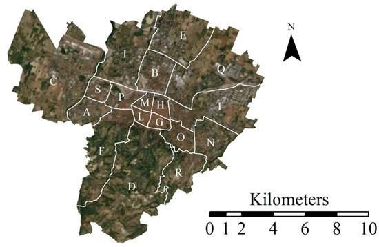
Figure 1.
Bologna case study with district boundaries and codes, assigned in alphabetical order.
2.2. Methodological Approach
The proposed methodological approach to map and assess supply and demand mismatches builds on existing literature on the topic [18,19,28,29]. The underlying idea is that cities not only benefit from ESs, but they also have a strong influence in their determination. Cities affect both ES supply (provision of the service that depends on the ecological structure of the city, on the presence of the ecosystem, its quality, and its location [9]) and demand, linked to social needs, according to the distribution, the demographic and the socioeconomic condition of the population, and current law requirement and standards of the investigated area, e.g., city’s air quality condition [9].
By tailoring and building upon existing methods, we propose a comprehensive approach to map and assess the supply and demand of three ESs—water retention and runoff, PM10 removal, and carbon storage and sequestration—in cities, with the aim of highlighting matches and mismatches between the assessed supply and demand. The methods chosen to map and assess regulating ecosystem services mostly follow a spatial proxy approach [30], using land use categories and derived data to assess ES supply and associating ES demand variables.
Based on the results of the supply and demand assessment, this work proposes a method to cluster urban areas into four categories by identifying for each a level of priority of policy intervention (high, medium, and low) and the possible nature-based solutions to be implemented to improve the sustainability of those areas.
2.2.1. Water Retention Supply and Demand Mapping and Assessment
Water retention is the regulating service based on the water cycle. Water resources, which are already under severe pressure in several regions of the world, are facing the worsening of their condition due to climate change. For this reason droughts, floods, storms, and related catastrophes will become even more critical [31,32]. The Local Climate Profile of Bologna [33], showing the current situation of the city and the future scenarios for climate, demonstrates that future precipitation will decrease during spring and winter, and during summer the number of days without rain will increase, as will the frequency of days with intense events. Therefore, water scarcity and hydrogeological instability are identified as critical issues. For this reason, the assessment of water retention supply is crucial.
Few methods exist based on detailed city water bulletins [19] that are not available in Bologna. For the purpose of this study, the supply of water retention is assessed as the change of water in storage or infiltration [19,28] within the city boundaries, and is computed as a percentage of total precipitation [29]. Infiltration rates related to land use categories (Winf—Table 2 of [29]) are applied to total annual precipitation (P) [34] in the city (Equation (1)).
S [mm] = P [mm] · Winf [%],
Subsequently, the supply computed for each land use is distributed over the districts’ areas; the supply of water per district was evaluated as the weighted average of infiltrated water per land use over the district (Equation (2)).
The demand for water (Equation (3)) is considered as the total amount of water consumed for different purposes within the city [19].
D [mm] = Dres + Dagr + Dair + Dind,ter,
Specifically:
- Residential demand (Equation (4)): water for domestic use. Population per district (Pop) [35] is multiplied by domestic water consumption per inhabitant (Wres) [36] and then distributed over the residential areas of each district (our computation based on [27]).
- Agricultural demand (Equation (5)): water needed to irrigate cultivated fields. The percentage of the cultivated area in need of irrigation (Acrop · %irrig) [37] is multiplied by the volume of water needed for the specific crop (Wcrop). Subsequently, agricultural demand is distributed over the agricultural areas (Acrop) (our computation based on [27]).
- Airport demand (Equation (6)): the airport’s total consumption of water (Waitport) [38] is distributed over its area (Aairport) (our computation based on [27]).
- Ecological demand (Equation (7)): all the resources used to water public parks, more generally, herbaceous green areas. The volume of water (Weco) [22] is distributed over parks, villas, and green areas associated with the road network (Apark) (our computation based on [27]).
- Industrial and tertiary demand (Equation (8)): computed as the difference between the volume of water consumed for nondomestic use (Dnon-dom) [36] and the abovementioned demands (Equations (5)–(7)).
The demand is subsequently distributed over the districts’ areas; demand of water per district (Equation (9)) is evaluated as the weighted average of different demands per land use over the district.
2.2.2. PM10 Removal Supply and Demand Mapping and Assessment
Air pollution can lead to negative effects in numerous sectors, as human health, economy, ecosystems, climate change, buildings, and artworks [39]. Specifically, PM10 is a “complex mixture of solid and liquid particles of organic and inorganic substances suspended in the air” [40] and is the pollutant that mostly affects human health, causing from asthma to lung cancer, and increases predisposition to respiratory diseases [40]. During 2016, it was estimated that 4.2 million premature deaths per year can be imputed to ambient air pollution [41,42]. Furthermore, numerous recent studies are investigating the influence of pollutants over COVID-19 spread and mortality rates, demonstrating the existence of a connection and thus identifying a new risk caused by air pollution [43,44,45,46,47]. Trees and herbaceous areas can contribute to the reduction of PM10 in air, thus improving overall air quality in the city [48,49,50,51].
Specifically, the supply of PM10 removal from urban ecosystems (Equation (10)) can be computed applying PM10 removal rates (RRPM10) to tree canopy cover (ATCC) and grass cover (AGC) [9,43,47]. Within this study, tree canopy cover (ATCC) and grass cover (AGC) were obtained through the i-Tree canopy tool [52,53].
The demand (Equation (11)) was considered as the current PM10 concentration (PM10,conc) [54], multiplied by the mixing height (MH) of 200 m [28,49]. This method was preferred to the possibility of considering PM10 concentration law limits as demand [18], since the main purpose of this study is to deepen the contribution of ESs in achieving the existent situation in Bologna.
For PM10 removal, air quality improvement (AQI) was also computed to identify an immediately understandable indication of trees and grass effectiveness and for comparison with other studies [18,49]. AQI (Equation (12)) was quantified as the PM10 removed (which in this analysis coincides with the supply) divided by the sum of the present PM10 (which in this analysis coincides with the demand) and PM10 removed (based on [49]).
2.2.3. Carbon Sequestration Supply and Demand Mapping and Assessment
Carbon dioxide (CO2) has always been present in atmosphere as a trace gas and necessary for the development of life, enabling photosynthesis and being a greenhouse gas (GHG) that traps infrared radiation. However, the excessive increase of GHG due to human activities brought dramatic changes in the carbon cycle and in the terrestrial balance, drastically contributing to climate change [55,56]. The latter already has observable and measurable effects on the environment—in 2018 the temperature had risen 0.99 ± 0.13 °C compared to the preindustrial years (1850–1900) [57], causing decrease of Arctic Sea ice, decrease of land ice sheets, increase of sea level, and more intense heat waves [58]. Currently, mitigating actions are a topic of great debate [59] and solutions should also be found within urban contexts, since cities are responsible for 75% of global CO2 emissions [60].
Carbon sequestration can be defined as the direct removal of CO2 over a period of time [55], while carbon storage is the overall CO2 that an ecosystem can store. Therefore, carbon storage values are absolute (i.e., not distributed over a period of time) and not comparable to other values of ESs supply and demand. Carbon storage was therefore excluded from this assessment.
Carbon sequestration supply (Equation (13)) is computed by applying carbon removal rates (RRCO2) [28,61] to tree canopy cover (ATCC). For this assessment, only the supply provided by trees was accounted, since there are no values in literature that confirm carbon sequestration by grass or bare soils [48].
The demand (Equation (14)) was estimated by considering the CO2 emissions per m2 produced in Bologna in 2018 [62]. As for PM10, emissions law limits could have been used as demand [18], but the study’s main purpose was to analyze the city’s current situation; factual emissions were considered.
2.2.4. ESDR and Districts’ Clusters: Identifying and Highlighting Mismatches for ESs
Within this study, we refer to the operational framework developed by Li et al. [63] and Chen et al. [19] to evaluate mismatches between ES supply and demand, and to further inform planning and management decisions on the basis of the relationships and the spatial distribution of ES supply and demand. ES mismatches reveal unsustainable uptake of ES expressed though unsatisfied demand for ES [64]. Therefore, an ES mismatch can be defined as the differences in quality or quantity occurring between the capacity, flow, and demand of ES [65]. Operationally, after having mapped and assessed supply and demand of the selected ESs, the ecosystem supply–demand ratio (ESDR, dimensionless parameter) [19] was evaluated for each ES assessed for the 18 city districts considered (Equation (15)).
This parameter has two main functions:
- It enables evaluation of the ratio between supply and demand within selected districts. If ESDR is greater than zero, an ecosystem service surplus is observed, and the demand is matched by the current supply; otherwise, if ESDR is negative, the supply cannot meet the demand, highlighting the shortage in the distribution of such service.
- It enables the comparison of different districts [63] through the creation of a scale composed by comparable dimensionless values.
The ESDR values obtained through the calculation described in (Equation (15)) are indicators of ES mismatches and can be used to cluster the districts into different classes presenting similar ES mismatches or performances. In order to define the priority of intervention by contemplating the ESs considered, ESDR classes referring to the three different mapped parameters per district were summed to obtain a representation of their overall condition.
According to the values obtained, we propose to group districts into four different classes to define priority (very high, high, medium, and low) and types of interventions (nature based solutionsNBS needed to improve current situation) within urban area. In addition, we propose to associate the ESDR classes with the proportion of land use within those districts (built-up and sealed, or green urban areas) and relevant tree canopy cover identified with i-Tree, thus relating priority and types of intervention with easy to assess characteristics of land use.
2.3. Data Collected
2.3.1. Water Retention
The supply computation is based on a similar study implemented in Munich [29] in which infiltration rates (Winf) were estimated per type of land cover as percentages of total annual precipitation (Table 2 of [29]). In this study, the total annual precipitation in Bologna was acquired from the metropolitan city web portal, through the statistical data section [36]. The precipitation value used refers to 2018, since more recent data were not available. In the city, two weather stations with rain gauges are available: one in Borgo Panigale district (646.6 mm) and one in Saffi district (772.0 mm). The mean value (709.3 mm) was assigned as constant precipitation for all the districts. As noted in Section 2.2.1, water retention demand was related to residential, agricultural, ecological, airport, and industrial utilization:
- Residential demand. The total population per district was acquired from the metropolitan city of Bologna web portal (population section) [35]. In addition, water for domestic use was retrieved from the open data website of the municipality, through an HERA-developed analysis [36]. The total consumption of water for domestic use in Bologna was observed to be of 21,710 · 103 m3/year during 2018. The data were then divided by the number of inhabitants of the city to determine the domestic water use per capita (m3/(year⋅inhabitant).
- Agricultural demand. All of the data noted were retrieved from a study developed by ISTAT (Italian National Institute of Statistics) [37] that provides irrigation volumes used by type of cultivation in cubic meters per hectare of irrigated area, and the area of irrigated surface as a percentage of the total agricultural area.
- Airport demand. The airport contribution to the overall request for water in Bologna comes from the sustainability report of the airport [38] and is referred to 2014. The proposed value is considered to be higher than more recent ones, since measures to contain water consumption at the airport were activated in the last few years [66] and is therefore considered an acceptable appraisal.
- Ecological demand. The ecological requested water for green urban areas (Weco) was retrieved from the Bologna Adaptation Plan [22] and are assumed to be stable for 2018.
- Industrial demand. Since no data were available for industrial consumption, the approach described in Section 2.2.1 was followed, and the total water for nondomestic use was retrieved from the previous HERA-developed analysis [36].
Even though the airport and the ecological water demand refer to 2014 and 2015, we assume that variation in the consumption of these two sectors would not affect the overall results.
2.3.2. PM10 Removal
In this assessment, both tree canopy cover and herbaceous cover were considered in order to calculate particulate matter reduction. The PM10 removal rate used for tree canopy cover (2.73 g/m2 per year) is proposed by Geneletti et al. [9] as assessed by Nowak and Crane [61]. On the other hand, the removal rate for grass cover was estimated to be 1.09 g/m2 per year, gained by dividing tree canopy removal rate by 2.5, as explained in Escobedo et al. [67,68]. Concerning PM10 demand, data concerning PM10 concentrations are openly accessible through the web portal of the metropolitan city—air quality section [54] and are collected by ARPAE, the Emilia-Romagna regional agency for prevention, environment, and energy. There are three air quality monitoring stations in Bologna (Figure 2) that gather data on PM10 concentration, which reported a daily mean value of 24 μg/m3 for 2018.
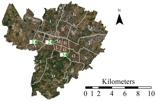
Figure 2.
Air quality monitoring network of Bologna.
2.3.3. Carbon Sequestration
Supply computation was developed by considering a CO2 removal rate of 1100 μg/m3 provided by tree canopy cover [28,61]. For the demand, no data on emissions in the atmosphere are available at the city level. Therefore, CO2 emissions in the metropolitan area of Bologna were considered, as developed by ARPAE and Regione Emilia-Romagna in the project INEMAR-ER [62].
3. Results
3.1. Water Retention Results
Annual values of infiltration (water retention supply) related to land use (Figure 3) vary from 5 mm in totally sealed areas (such as roads and compact residential fabric) to 380,894 mm in pervious areas (such as railways).
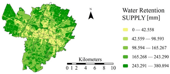
Figure 3.
Water retention supply per land use.
As clearly shown already in Figure 3 and then represented in an aggregated manner in Figure 4, the historical districts located in the center of the urban area of Bologna are reporting the lowest supply in terms of runoff control and water retention, as they represent the most sealed areas of the city. This could lead to flash flood events in the city centers, due to the heavy rains from which the areas are currently suffer. In line with Pauleit et al. [29], most peripheral areas north, east, and south of the city center present much higher value of runoff control, because these areas are mostly covered by either agricultural land or urban forest and significantly contribute to groundwater recharge in the urban areas.
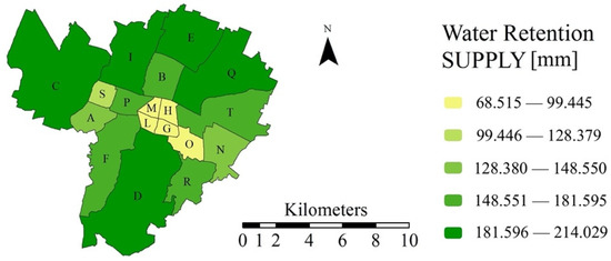
Figure 4.
Water retention supply per district.
The consumption of water (water retention demand) varies from a minimum of 0 mm (for wooded areas) to a maximum of almost 1350 mm (for domestic use in the most populated districts) (Figure 5 and Figure 6).
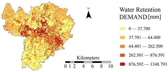
Figure 5.
Water retention demand per land use.
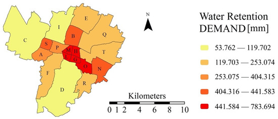
Figure 6.
Water retention demand per district.
Comparing supply and demand spatial values through ESDR (Figure 7), it can be observed that shortfalls (ESDR < 0) decrease and cease to exist when moving from the center towards the suburban areas. This is clearly related to the highest density of population and imperviousness in the most central neighborhoods [25]. The districts located in the city center, with the highest number of residents and thus densely inhabited and sealed land, are the ones requesting more water, mostly for domestic uses. These areas also account for the lowest water retention supply, thus presenting the highest supply–demand mismatch of the city. Districts around the city center heading east and west also present high ESDR values. These districts are predominately residential areas, thus requesting high amounts of water for domestic use and mostly sealed with residential houses and services. Areas at the north and south of the city that present low or no mismatches correspond to the wooded areas of the city (F and D) or include an high amount of pervious areas (i.e., agricultural areas, underused land, vacant land).
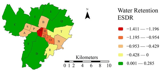
Figure 7.
Water retention ESDR.
3.2. PM10 Removal Results
During 2019, the annual average concentration of PM10 in Bologna was 26 μg/m3 [69], compliant with the annual limit value of 40 μg/m3 imposed by European directive 1999/30/EC [70], which was incorporated into Italian legislation via Legislative Decree 60/2002 [71]. However, the WHO air quality guidelines propose a limit of 20 μg/m3 [72]. In 2019, one of the meteorological stations of Bologna (Porta San Felice) registered 32 days exceeding the 24-h limit of 50 μg/m3 [73], close to the limit of 35 days per year [71]. Even if measures to reduce air pollution are in action in the city (implementation of green areas, strengthening of soft mobility, limitations to urban traffic, promotion of electric and hybrid vehicles, among others [74]), the situation is still critical. As shown in the methodological approach (Section 2.2.2), the current PM10 concentration was considered to represent the demand situation in Bologna, providing a spatially uniform demand of 42,048 g/(m2∙year).
PM10 removal supply results in Figure 8 present the same classification of districts as the one representing analyzed air quality improvement (Figure 9). However, through AQI computation it is possible to observe that trees in Bologna provide an air quality improvement that ranges from 0.5% and 2.5%, in line with previous studies [18].
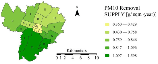
Figure 8.
PM10 removal supply.
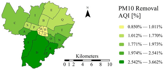
Figure 9.
Air quality improvement (AQI) for particulate matter.
According to both the computed values and the ones sourced in scientific literature, AQI by trees and grass has a limited impact on PM10 removal and presents modest effects on achieving compliance to limits and guidelines [18].
Concerning PM10 removal distribution around the city (Figure 10), as already described for runoff regulation, districts located in south areas of the city have a major positive impact over the air quality improvement, since they are mostly covered by urban forest—completely wooded areas with values up to 100% of tree canopy coverage (TCC). The historical city center (districts G, H, L, and M) shows the lowest supply, and thus the largest mismatches in terms of ESDR over the entire city. City center districts present both low values of TCC and of green areas. The northern areas of the city, which perform well in terms of water retention, present high mismatches in air quality regulation.
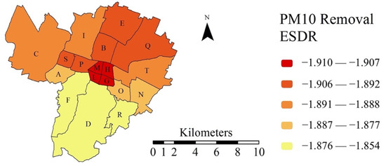
Figure 10.
PM10 removal ESDR.
3.3. Carbon Sequestration Results
As for PM10 removal, while carbon sequestration supply varies for each district (Figure 11), the demand is calculated with a spatially uniform value of emissions in the city (1559.816 g/(m2∙year)). As for carbon sequestration supply, Figure 11 shows carbon sequestration values in terms of g/(m2∙year) and presents some interesting differences with the previous PM10 supply assessment. Indeed, wider variation is presented in the different areas of the city, depending on the number of trees and related TCC. The historical city center, for instance, presents different values among its districts, since district H hosts the biggest and most historical park of the city (Parco della Montagnola), the University Botanical gardens, and many tree-lined avenues. On the other side, district C, located at the far west of the city belongs to the worst performing class since it is mostly an agriculturally based district, with limited TCC area.
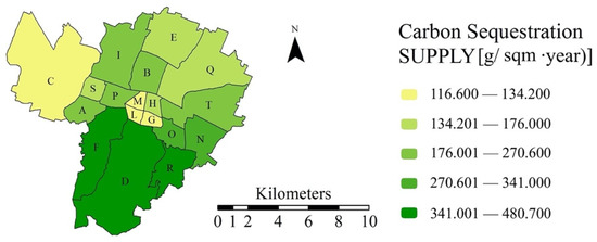
Figure 11.
Carbon sequestration supply.
As for PM10, the carbon sequestration ESDR mismatches map corresponds to the supply map, since demand data have been equally distributed around the city. Only three districts belonging to the city center show the lowest ESDR (Figure 12). In fact, district H presents a moderately better condition that is due to the presence of one of the largest urban parks of Bologna. In addition, district C is characterized by the lowest ESDR class, since it has a multitude of green and agricultural fields, but there are hardly any trees. Districts in the hill and woodland areas of the city still reveal the smallest mismatches because of their numerous wooded areas.
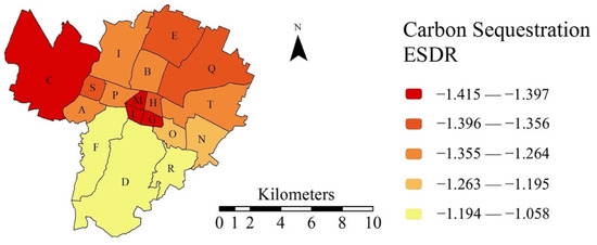
Figure 12.
Carbon sequestration ESDR
3.4. Clustering of Districts
For the three ES considered, a value from 1 (lowest ESDR, poorest condition) to 5 (highest ESDR, best condition) was assigned to each district using an ArcGIS normalization algorithm package. The values obtained, corresponding to the overall performance of each district in relation with the three ES considered, were used to classify the district in four classes, as illustrated in Figure 13.
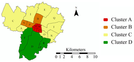
Figure 13.
Clustering of districts.
This characterization allows for the identification of four classes of districts with similar characteristics of land use and TCC, and related performance in relation with the three ES considered. As Table 1 summarizes, the ratio of predominant land use (Built-Up and Sealed - BUS, and Urban Green Areas - UGA) and TCC can be considered as a proxy for water retention, PM10 removal, and carbon sequestration in urban areas. The first class, cluster A (see Table 1 and Figure 13), within our case study corresponds to districts belonging to the city center with value of BUS land higher than 95% and TCC below 15%. Since these areas present the highest ESDR mismatches for the the ES assessed, the priority for intervention has been recognized here as very high. The second class still presents a high range of BUS land (not less than 80%) with a low percentage of TCC (ranging from 15% to 25%). This cluster still shows large mismatches in all the ES, thus the priority of intervention remains high. Cluster C includes the higher variability districts, including those with very different characteristics, as BUS ranges from 40% to 85% and UGA up to 60%, with still a limited value of TCC (up to 35%). This cluster presents the widest variation of performance of the three ES, thus priority of intervention is considered as medium and should refer to the main mismatches identified in the analysis of the individual ES. Last, the fourth group (cluster D) includes the districts with the lowest or no ESDR mismatches, corresponding to the hilly and wooded forest of the city. This cluster does not need any intervention concerning the three ES assessed in this work.

Table 1.
City districts and priority of intervention clustered according to percentage of built-up and sealed (BU), green urban areas (GUA) and tree canopy cover (TCC).
4. Discussion
Concerning water retention supply, and according to similar studies (see [20]), the peripheral districts had clearly higher supply performances than the city center, and, at the same time water demand was more clustered in the city center because of the higher population numbers and density. This led to high shortfalls and negative supply–demand and it could be associated with floods and flash floods taking place within the city center at an increasingly frequent rate due to climate change. Considering the high rate of population living in the city center, such floods can greatly affect the urban system, provoking economic, social, and environmental damages. Acknowledging difficulties in desealing historical and compact city centers, several solutions could be put in place: permeable paving systems could be promoted and incentivized for parking lots and nonhistorical squares [75,76], further soil sealing should be banned and green roofs and walls with high rates of water retention, where possible due to heritage constraints, should be implemented, and incentivized in public and private buildings [75]. In addition, initiatives to reduce the consumption of water and enhance wastewater reuse should be encouraged.
Looking at PM10 removal, results are in line with similar studies. Nowak et al. [49] found that AQI went from 0.2% to 1.0% in different cities of the United States during 1994 and Barò et al. [18] observed the range 0.5–1.89% in five European cities in 2011. Even though the results of this study are a slightly higher than the ones found in literature, we still recognized that air quality improvement by trees and grass has a limited impact on PM10 removal and presents modest effects on achieving compliance to limits and guidelines. Despite this, there is evidence that benefits in human health and wellbeing can be seen with almost any decrease in PM10 concentrations [40].
As for carbon sequestration, our study confirms that the contribution of urban forests to regulate CO2 emission is substantial in absolute terms, yet modest when compared to overall city levels of GHG emissions [50]. Nevertheless, urban green spaces can play an important role as carbon sinks (e.g., Nowak et al. [77]) and carbon sequestration rates are in some cases comparable to other local mitigation strategies based on energy savings [78]. At the same time, such nature-based solutions provide a wide range of cobenefits (i.e., water regulation and PM10) not treated in this study (noise reduction, recreational services, microclimate regulation), but still relevant in terms of land use and planning decision-making processes. Planting trees in dense sealed and built-up areas, or greening bare soil and abandoned areas should be promoted, and it should be wisely planned in terms of species that could increase current canopy cover and could adapt to future climate projections or a better selection of species and crown diameters [79,80,81]. In the case of a lack of available and unoccupied areas, the positive contribution of green roofs [76,77] and green walls [78,79] should be considered and incentivized.
In addition, the identification of four clusters of districts based on their predominant land use and TCC allows for the identification of a similar pattern of performances throughout the city. This information can be relevant for planners and decision makers in the development of the city master plans or local action plan for climate mitigation and adaptation.
Specifically, districts presenting more than 95% built-up and sealed land with less than 15% of TCC have been framed within the highest priority cluster area. These urban areas are densely built and inhabited, and lack available space. Therefore, hybrid nature-based solutions (NBS) should be considered as the intervention first proposed for improving the local situation. Specifically, even acknowledging the difficulties in desealing historical and compact city centers, permeable paving systems should be promoted and incentivized for parking lots and nonhistorical squares, further soil sealing should be avoided and green roofs and walls with high rate of water retention, where possible, should be implemented and incentivized in public and private buildings [75]. Additionally, initiatives to reduce the consumption of water and enhance wastewater reuse should be encouraged and incentives for private greening initiatives can be considered.
On the other side, districts that have a range of built-up and sealed areas from 85% to 95% and a TCC from 15% to 25% have been classified in cluster B, suggesting high priority of intervention. For districts falling in this cluster, the proposed strategy would be shortfall-oriented. Despite the high share of built-up areas, the overall condition of these areas is not as poor as for the ones in cluster A, thanks to the higher presence of trees. Nevertheless, actions and measures aimed at increasing water retention should be sought, to avoid water runoff and mitigating the risk of flood and flash floods. Hybrid interventions such as green roofs and walls are highly recommended in this area, which, at least in the case of Bologna, also present fewer heritage constraints and could undertake heavier regeneration interventions on private and public buildings.
Districts falling in cluster C present variable values of built-up and sealed land (ranging from 40% to 85%) and values of TCC ranging from 10% to 35%. Even though the overall ES performance in these districts can be generally acceptable, these districts, as in the case of Bologna, could present higher rates of vacant or underused land. For this reason, cluster C could undertake more drastic and decisive interventions contributing to improve the overall performance of the city. Districts belonging to this cluster provide the greatest opportunity for green urban regeneration projects. Indeed, the presence of vacant land, urban voids, building demolition and replacement projects, etc., raises the possibility to design new multifunctional NBSs (urban parks, watercourses to draw new ecological systems or creating new community gardens [80,81,82], and ecological corridors), based on the actual main challenges of the area (i.e., water retention, PM10 concentration, urban heat island, no open green public space available). These nature-based interventions would largely contribute to improved quality of life and health of citizens living in these districts. Even if not in the main purpose of this study, it must be highlighted that within this cluster there is a high potential for increasing recreational and cultural services. Finally, districts with TCC values over 35% and less than 50% of built-up and sealed areas have been clustered in cluster D, which present the lowest priority of intervention.
These districts present surpluses of water retention ES and show values of PM10 removal and carbon sequestration that are comparable to the highest found in literature for other cities (e.g., Salzburg and Stockholm) [19,44,46,81]. This consideration does not exclude further interventions, but aims at highlighting that operations in this area could have a lower priority in urban strategies and policy making.
Promoting the introduction of ESs into urban plans and strategies, this approach has some limitations that need to be considered: (1) Ecological coefficients were taken from studies conducted in other cities, but with characteristics similar to Bologna. Even if this does not significantly affect the final classification, more accurate evaluations should be considered for further investigation if specific coefficients are estimated for the city of Bologna. (2) The influence area of ecosystems was considered to be the district’s boundary. (3) The accuracy of the results can vary with the operator’s precision while interpreting the possible ambiguities of Google aerial images though i-Tree Canopy. In addition, the spatial proxy methods used to compute and map regulating ecosystem services in the city strictly depend on available data and the dataset, so careful attention should be devoted to the step of data acquisition and elaboration.
5. Conclusions
Even though more complex mathematical modeling, remote sensing data, and direct field observation and measurement can provide more reliable outcomes in terms of ES quantification, spatial proxy methods are considered adequate in the scope of this work since they contributed to:
- (i)
- Identifing “hotspot” areas with high mismatches of ES supply and demand;
- (ii)
- Enhancing engagement of stakeholders in the codevelopment and coimplementation of relevant measures to address mismatches;
- (iii)
- Supporting decision-makers in setting priorities by communicating the overall benefits and shortcomings through easy-to-read maps of the city;
- (iv)
- Classifying and clustering urban areas, i.e., districts, that present similar results in terms of mismatches for ES supply and demand, and further define priority and type of intervention;
- (v)
- Potentially enhancing citizens’ valuation of ecosystem services, providing them with a clear understanding of ES benefits derived and raising awareness among the population on the relevance of the urban green and blue infrastructures (GBI).
The degree of accurateness used to build ES maps and the selection of methods and indicators applied, lies in the need, within this work, not to advance in terms of modeling and quantification methods, but rather to propose a spatially based approach to evaluate ES deficit or surpluses within urban areas, thus supporting local planners and decision makers. Through the methodological approach for assessing and mapping the supply and demand of the three ecosystem services studied (water retention, PM10 removal, and carbon sequestration), this study identified four categories of city districts based on UESs mismatches and linked to different priority of intervention levels, which contributes to the current discussion on the use of ES in planning [82].
While the results presented in this study can already provide some useful insights to planners of urban areas similar to the case presented, further research should be focused on testing the proposed methodology in different cities, enhancing the integration of UESs in urban planning, and finding strategies to achieve better life conditions, health, and wellbeing.
Author Contributions
Conceptualization, C.d.L.; methodology, F.V. and C.d.L.; validation, S.T.; formal analysis, F.V.; investigation, F.V.; data curation, F.V.; writing—original draft preparation, F.V.; writing—review and editing, C.d.L.; visualization, F.V.; supervision, S.T. All authors have read and agreed to the published version of the manuscript.
Funding
This research received no external funding.
Data Availability Statement
The data presented in this study are available on request from the corresponding author. Some of the data are not publicly available due to the mixed origins and availability. Some of the database used are directly available from the list of references.
Conflicts of Interest
The authors declare no conflict of interest.
References
- United Nations: Department of Economic and Social Affairs. Population Division. World Urbanization Prospects 2018: Highlights; United Nations: New York, NY, USA, 2019; ISBN 978-92-1-148318-5. [Google Scholar]
- EEA. The European Environment—State and Outlook 2020. Knowledge for Transition to a Sustainable Europe; 2019; ISBN 978-92-9480-090-9. Available online: https://www.preventionweb.net/publications/view/69423 (accessed on 3 September 2020).
- Elmqvist, T.; Goodness, J.; Marcotullio, P.J.; Parnell, S.; Sendstad, M.; Wilkinson, C.; Fragkias, M.; Güneralp, B.; McDonald, R.I.; Schewenius, M.; et al. Urbanization, Biodiversity and Ecosystem Services: Challenges and Opportunities: A Global Assessment; Springer: Dordrecht, The Netherlands, 2013; ISBN 978-94-007-7088-1. [Google Scholar]
- Cortinovis, C.; Geneletti, D. Ecosystem Services in Urban Plans: What Is There, and What Is Still Needed for Better Decisions. Land Use Policy 2018, 70, 298–312. [Google Scholar] [CrossRef]
- McPhearson, T.; Andersson, E.; Elmqvist, T.; Frantzeskaki, N. Resilience of and through Urban Ecosystem Services. Ecosyst. Serv. 2015, 12, 152–156. [Google Scholar] [CrossRef]
- MEA. Millennium Ecosystem Assessment: Ecosystems and Human Well-Being—A Framework for Assessment; Island Press: Washington, DC, USA, 2003. [Google Scholar]
- Fisher, B.; Turner, R.K.; Morling, P. Defining and Classifying Ecosystem Services for Decision Making. Ecol. Econ. 2009. [Google Scholar] [CrossRef]
- Millennium Ecosystem Assessment. Ecosystems and Human Well-Being. Synthesis; Island Press: Washington, DC, USA, 2005; ISBN 1-59726-040-1. [Google Scholar]
- Geneletti, D.; Cortinovis, C.; Zardo, L.; Esmail, B.A. Planning for Ecosystem Services in Cities, 1st ed.; Springer International Publishing: Cham, Switzerland, 2020; ISBN 978-3-030-20023-7. [Google Scholar]
- Bolund, P.; Hunhammar, S. Ecosystem Services in Urban Areas. Ecol. Econ. 1999, 29, 293–301. [Google Scholar] [CrossRef]
- Haase, D.; Larondelle, N.; Andersson, E.; Artmann, M.; Borgström, S.; Breuste, J.; Gomez-Baggethun, E.; Gren, Å.; Hamstead, Z.; Hansen, R.; et al. A Quantitative Review of Urban Ecosystem Service Assessments: Concepts, Models, and Implementation. Ambio 2014, 43, 413–433. [Google Scholar] [CrossRef]
- Gómez-Baggethun, E.; Barton, D.N. Classifying and Valuing Ecosystem Services for Urban Planning. Ecol. Econ. 2013, 86, 235–245. [Google Scholar] [CrossRef]
- TEEB. The Economics of Ecosystems and Biodiversity Ecological and Economic Foundations; Earthscan: London, UK; Washington, DC, USA, 2010. [Google Scholar]
- Hansen, R.; Frantzeskaki, N.; McPhearson, T.; Rall, E.; Kabisch, N.; Kaczorowska, A.; Kain, J.-H.; Artmann, M.; Pauleit, S. The Uptake of the Ecosystem Services Concept in Planning Discourses of European and American Cities. Ecosyst. Serv. 2015, 12, 228–246. [Google Scholar] [CrossRef]
- Kaczorowska, A.; Kain, J.-H.; Kronenberg, J.; Haase, D. Ecosystem Services in Urban Land Use Planning: Integration Challenges in Complex Urban Settings—Case of Stockholm. Ecosyst. Serv. 2016, 22, 204–212. [Google Scholar] [CrossRef]
- Kabisch, N. Ecosystem Service Implementation and Governance Challenges in Urban Green Space Planning—The Case of Berlin, Germany. Land Use Policy 2015, 42, 557–567. [Google Scholar] [CrossRef]
- World Health Organization. Ecosystems and Human Well-Being—Health Synthesis. A report of the Millennium Ecosystem Assessment; WHO Press: Geneva, Switzerland, 2005. [Google Scholar]
- Baró, F.; Haase, D.; Gómez-Baggethun, E.; Frantzeskaki, N. Mismatches between Ecosystem Services Supply and Demand in Urban Areas: A Quantitative Assessment in Five European Cities. Ecol. Indic. 2015. [Google Scholar] [CrossRef]
- Chen, J.; Jiang, B.; Bai, Y.; Xu, X.; Alatalo, J.M. Quantifying Ecosystem Services Supply and Demand Shortfalls and Mismatches for Management Optimisation. Sci. Total Environ. 2019, 650, 1426–1439. [Google Scholar] [CrossRef] [PubMed]
- Atlante Statistico Metropolitano Studio Sul Movimento—Trend. Available online: http://inumeridibolognametropolitana.it/atlantemetropolitano/popolazione/movimento-della-popolazione/studio-sul-movimento (accessed on 8 May 2020).
- ARPA Lombardia Progetto Bacino Padano—Aria/Qualità Dell’Aria. Available online: https://www.arpalombardia.it:443/Pages/Aria/Aria-Progetti/Progetto-Bacino-Padano.aspx (accessed on 29 October 2020).
- Comune di Bologna Piano Di Adattamento Città Di Bologna. Available online: http://www.comune.bologna.it/media/files/piano_adattamento_bologna.pdf (accessed on 3 September 2020).
- De Luca, C.; Martin, J.; Tondelli, S. Ecosystem Services Integration into Local Policies and Strategies in the City of Bologna: Analysis of the State of the Art and Recommendations for Future Development. Ecosyst. Serv. Green Infrastruct. Cities Nat. 2021. [Google Scholar] [CrossRef]
- Comune di Bologna Iperbole—PSC. Available online: http://www.comune.bologna.it/psc/ (accessed on 20 October 2020).
- Copernicus Imperviousness Density. 2015. Available online: https://land.copernicus.eu/pan-european/high-resolution-layers/imperviousness/status-maps/2015 (accessed on 10 February 2020).
- Comune di Bologna PSC—Documenti di Piano—Figure Della Ristrutturazione. Available online: http://informa.comune.bologna.it/iperbole/psc/documenti/850 (accessed on 5 January 2020).
- Regione Emilia-Romagna Coperture Vettoriali Dell’uso Del Suolo—Edizione 2018. Available online: https://geoportale.regione.emilia-romagna.it/it/download/dati-e-prodotti-cartografici-preconfezionati/pianificazione-e-catasto/uso-del-suolo-1/2014-coperture-vettoriali-uso-del-suolo-di-dettaglio-edizione-2018/dati-preconfezionati (accessed on 11 November 2019).
- Larondelle, N.; Lauf, S. Balancing Demand and Supply of Multiple Urban Ecosystem Services on Different Spatial Scales. Ecosyst. Serv. 2016. [Google Scholar] [CrossRef]
- Pauleit, S.; Duhme, F. Assessing the Environmental Performance of Land Cover Types for Urban Planning. Landsc. Urban Plan. 2000. [Google Scholar] [CrossRef]
- Vihervaara, P.; Poikolainen, L.; Nedkov, S.; Viinikka, A.; Adamescu, C.; Arnell, A.; Balzan, M.; Bicking, S.; Broekx, S.; Burkhard, B.; et al. Biophysical Mapping and Assessment Methods for Ecosystem Services; Deliverable D3.3 EU Horizon 2020 ESMERALDA Project, Grant Agreement No. 642007, 2018. (EU Deliverable). Available online: https://www.researchgate.net/profile/Malgorzata_Stepniewska/publication/325217449_Biophysical_Mapping_and_Assessment_Methods_for_Ecosystem_Services/links/5afe971daca272b5d84ab65e/Biophysical-Mapping-and-Assessment-Methods-for-Ecosystem-Services.pdf (accessed on 3 September 2020).
- Water and Climate Change. Available online: https://www.iucn.org/resources/issues-briefs/water-and-climate-change (accessed on 20 October 2020).
- UNESCO; UN-Water. UN World Water Development Report 2020: Water and Climate Change; Water and Climate Change; UNESCO: Paris, France, 2020. [Google Scholar]
- Comune di Bologna; Kyoto Club; AmbienteItalia; ARPA BLUEAP. PROFILO CLIMATICO LOCALE: Analisi Delle Vulnerabilità All’impatto Dei Cambiamenti Climatici. Available online: https://docs.google.com/viewerng/viewer?url=http://www.blueap.eu/site/wp-content/uploads/2013/11/BLUEAP_PROFILO_CLIMATICO_LOCALE.pdf (accessed on 7 September 2020).
- Comune di Bologna Climatologia—Temperature e Precipitazioni. Available online: http://inumeridibolognametropolitana.it/dati-statistici/ambiente-e-territorio/climatologia (accessed on 20 January 2020).
- Comune di Bologna Popolazione Residente per Età, Quartiere e Zona al 31 Dicembre—Serie Storica. Available online: http://inumeridibolognametropolitana.it/dati-statistici/popolazione-residente-eta-quartiere-e-zona-al-31-dicembre-serie-storica (accessed on 20 January 2020).
- Comune di Bologna Acqua—Consumo Di Acqua per i Diversi Usi Nel Comune Di Bologna Dal 1996 al 2018. Available online: http://www.comune.bologna.it/iperbole/piancont/dati_statistici/Indici/Ambiente%20e%20territorio/index.htm (accessed on 11 September 2020).
- Istituto Nazionale di Statistica (ISTAT) Utilizzo e Qualità Della Risorsa Idrica in Italia. Available online: https://www.istat.it/it/files//2019/10/Utilizzo-e-qualit%C3%A0-della-risorsa-idrica-in-Italia.pdf (accessed on 11 September 2020).
- Aeroporto Guglielmo Marconi di Bologna S.p.A. Bilancio Di Sostenibilità. 2014. Available online: https://www.bologna-airport.it/System/files/Bilanciaziendali/bilancio_sostenibilita_2014.pdf (accessed on 19 December 2020).
- EEA; Guerreiro, C.; Ortiz, G.A.; de Leeuw, F. Air Quality in Europe—2017 Report; Publications Office of the European Union: Luxembourg, 2017; ISBN ISSN 1725-9177. [Google Scholar]
- WHO. Health Effects of Particulate Matter: Policy Implications for Countries in Eastern Europe, Caucasus and Central Asia. J. Korean Med Assoc. 2013. [Google Scholar] [CrossRef]
- World Health Organization Ambient (Outdoor) Air Pollution. Available online: https://www.who.int/news-room/fact-sheets/detail/ambient-(outdoor)-air-quality-and-health (accessed on 7 October 2020).
- World Health Organization. Air Pollution. Available online: https://www.who.int/westernpacific/health-topics/air-pollution (accessed on 7 October 2020).
- Hendryx, M.; Luo, J. COVID-19 Prevalence and Fatality Rates in Association with Air Pollution Emission Concentrations and Emission Sources. Environ. Pollut. 2020, 265, 115126. [Google Scholar] [CrossRef]
- Magazzino, C.; Mele, M.; Schneider, N. The Relationship between Air Pollution and COVID-19-Related Deaths: An Application to Three French Cities. Appl. Energy 2020, 279, 115835. [Google Scholar] [CrossRef]
- Yao, Y.; Pan, J.; Wang, W.; Liu, Z.; Kan, H.; Qiu, Y.; Meng, X.; Wang, W. Association of Particulate Matter Pollution and Case Fatality Rate of COVID-19 in 49 Chinese Cities. Sci. Total Environ. 2020, 741, 140396. [Google Scholar] [CrossRef]
- Zhang, Z.; Xue, T.; Jin, X. Effects of Meteorological Conditions and Air Pollution on COVID-19 Transmission: Evidence from 219 Chinese Cities. Sci. Total Environ. 2020, 741, 140244. [Google Scholar] [CrossRef] [PubMed]
- Zhu, Y.; Xie, J.; Huang, F.; Cao, L. Association between Short-Term Exposure to Air Pollution and COVID-19 Infection: Evidence from China. Sci. Total Environ. 2020, 727, 138704. [Google Scholar] [CrossRef]
- McPhearson, T.; Kremer, P.; Hamstead, Z.A. Mapping Ecosystem Services in New York City: Applying a Social-Ecological Approach in Urban Vacant Land. Ecosyst. Serv. 2013. [Google Scholar] [CrossRef]
- Nowak, D.J.; Crane, D.E.; Stevens, J.C. Air Pollution Removal by Urban Trees and Shrubs in the United States. Urban For. Urban Green. 2006. [Google Scholar] [CrossRef]
- Baró, F.; Chaparro, L.; Gómez-Baggethun, E.; Langemeyer, J.; Nowak, D.J.; Terradas, J. Contribution of Ecosystem Services to Air Quality and Climate Change Mitigation Policies: The Case of Urban Forests in Barcelona, Spain. Ambio 2014. [Google Scholar] [CrossRef]
- McPherson, G.E.; Nowak, D.J.; Rowntree, R.A. Chicago’s Urban Forest Ecosystem: Results of the Chicago Urban Forest Climate Project, 1st ed.; U.S. Department of Agriculture, Forest Service, Northeastern Forest Experiment Station: Radnor, PA, USA, 1994. [CrossRef]
- i-Tree Cooperative I-Tree Canopy. Available online: https://canopy.itreetools.org/ (accessed on 3 October 2020).
- Nowak, D.J.; Crane, D.E. The Urban Forest Effects (UFORE) Model: Quantifying Urban Forest Structure and Functions. In Integrated Tools for Natural Resources Inventories in the 21st Century; Gen. Tech. Rep. NC-212; Mark, H., Tom, T., Eds.; Dept. of Agriculture, Forest Service, North Central Forest Experiment Station: St. Paul, MN, USA, 2000; Volume 212, pp. 714–720. [Google Scholar]
- Comune di Bologna Qualità Dell’aria. Available online: http://inumeridibolognametropolitana.it/dati-statistici/ambiente-e-territorio/qualita-dellaria (accessed on 9 September 2020).
- IPCC. Climate Change 2013: The Physical Science Basis. Contribution of Working Group I to the Fifth Assessment Report of the Intergovernmental Panel on Climate Change; Cambridge University Press: Cambridge, UK, 2013; p. 1535. [Google Scholar]
- Lindsey, R. Climate Change: Atmospheric Carbon Dioxide. Available online: https://www.climate.gov/news-features/understanding-climate/climate-change-atmospheric-carbon-dioxide (accessed on 10 September 2020).
- World Meteorological Organization. WMO Statement on the State of the Global Climate in 2018; World Meteorological Organization (WMO): Geneva, Switzerland, 2019. [Google Scholar]
- NASA Global Climate Change Carbon Dioxide Concentration | NASA Global Climate Change. Available online: https://climate.nasa.gov/vital-signs/carbon-dioxide (accessed on 7 October 2020).
- Intergovernmental Panel on Climate Change (IPCC); Pachauri, R.K.; Allen, M.R.; Barros, V.R.; Broome, J.; Cramer, W.; Christ, R.; Church, J.A.; Clarke, L.; Dahe, Q.; et al. Climate Change 2014: Synthesis Report. Contribution of Working Groups I, II and III to the Fifth Assessment Report of the Intergovernmental Panel on Climate Change; Pachauri, R.K., Meyer, L.A., Eds.; IPCC: Geneva, Switzerland, 2014. [Google Scholar]
- Environment Programme, U.N. Cities and Climate Change. Available online: http://www.unenvironment.org/explore-topics/resource-efficiency/what-we-do/cities/cities-and-climate-change (accessed on 7 October 2020).
- Nowak, D.J.; Crane, D.E. Carbon Storage and Sequestration by Urban Trees in the USA. Environ. Pollut. 2002, 116, 381–389. [Google Scholar] [CrossRef]
- ARPAE; Regione Emilia-Romagna Aggiornamento Dell’inventario Regionale Delle Emissioni in Atmosfera Dell’Emilia-Romagna Relativo All’anno 2015 (INEMAR-ER 2015). Available online: https://www.google.com/url?sa=t&rct=j&q=&esrc=s&source=web&cd=&ved=2ahUKEwirzKK465TvAhUFOuwKHRMLCrsQFjABegQIAxAD&url=https%3A%2F%2Fwww.arpae.it%2Fit%2Ftemi-ambientali%2Faria%2Finventario-emissioni%2Finventario_emissioni_2017.pdf&usg=AOvVaw1eVBduuK69rCJHKvpjm00T (accessed on 10 September 2020).
- Li, J.; Jiang, H.; Bai, Y.; Alatalo, J.M.; Li, X.; Jiang, H.; Liu, G.; Xu, J. Indicators for Spatial-Temporal Comparisons of Ecosystem Service Status between Regions: A Case Study of the Taihu River Basin, China. Ecol. Indic. 2016. [Google Scholar] [CrossRef]
- Baró, F.; Palomo, I.; Zulian, G.; Vizcaino, P.; Haase, D.; Gómez-Baggethun, E. Mapping Ecosystem Service Capacity, Flow and Demand for Landscape and Urban Planning: A Case Study in the Barcelona Metropolitan Region. Land Use Policy 2016, 57, 405–417. [Google Scholar] [CrossRef]
- Geijzendorffer, I.R.; Martín-López, B.; Roche, P.K. Improving the Identification of Mismatches in Ecosystem Services Assessments. Ecol. Indic. 2015, 52, 320–331. [Google Scholar] [CrossRef]
- Ambiti Di Attività - Aeroporto G. Marconi Di Bologna BLQ. Available online: https://www.bologna-airport.it/la-societa/ambiente-qualita-e-sicurezza/ambiente-ed-energia/i-nostri-ambiti-di-attivita/?idC=62379 (accessed on 19 December 2020).
- Escobedo, F.J.; Wagner, J.E.; Nowak, D.J.; De la Maza, C.L.; Rodriguez, M.; Crane, D.E. Analyzing the Cost Effectiveness of Santiago, Chile’s Policy of Using Urban Forests to Improve Air Quality. J. Environ. Manag. 2008. [Google Scholar] [CrossRef] [PubMed]
- Shreffler, J.H. Factors Affecting Dry Deposition of SO2 on Forests and Grasslands. Atmos. Environ. (1967) 1978. [Google Scholar] [CrossRef]
- Comune di Bologna Concentrazione Di Alcuni Inquinanti Nell’aria Rilevata Dalle Centraline Di Bologna. Valori Medi Annui - Serie Storica | I Numeri Di Bologna. Available online: http://inumeridibolognametropolitana.it/dati-statistici/concentrazione-di-alcuni-inquinanti-nellaria-rilevata-dalle-centraline-di-bologna (accessed on 29 October 2020).
- Council of European Union. Council Directive 1999/30/EC of 22 April 1999 Relating to Limit Values for Sulphur Dioxide, Nitrogen Dioxide and Oxides of Nitrogen, Particulate Matter and Lead in Ambient Air; Office for Official Publications of the European Communities: Luxembourg, 1999; Volume L 163, pp. 0041–0060. [Google Scholar]
- Ministero dell’Ambiente e della Tutela del Territorio (law). Recepimento Della Direttiva 1999/30/CE Del Consiglio Del 22 Aprile 1999 Concernente i Valori Limite Di Qualita’ Dell’aria Ambiente per Il Biossido Di Zolfo, Il Biossido Di Azoto, Gli Ossidi Di Azoto, Le Particelle e Il Piombo e Della Direttiva 2000/69/CE Relativa Ai Valori Limite Di Qualita’ Dell’aria Ambiente per Il Benzene Ed Il Monossido Di Carbonio; Ministry of Justice - Directorate of the Official Gazette of the Italian Republic: Rome, Italy, 2002.
- World Health Organization. Air Quality Guidelines. Global Update 2005; WHO Press: Geneva, Switzerland, 2006; ISBN 92 890 1358 3. [Google Scholar]
- Comune di Bologna Numero Di Giorni Di Superamento Del Limite Giornaliero Di PM10 Nell’aria Rilevata Dalle Centraline Di Bologna - Serie Storica | I Numeri Di Bologna. Available online: http://inumeridibolognametropolitana.it/dati-statistici/numero-di-giorni-di-superamento-del-limite-giornaliero-di-pm10-nellaria-rilevata (accessed on 29 October 2020).
- Regione Emilia-Romagna (law). Misure per Il Miglioramento Della Qualità Dell’aria in Attuazione Del Piano Aria Integrato Regionale (Pair 2020) e Del Nuovo Accordo Di Bacino Padano 2017; Redazione del Bollettino Ufficiale: Bologna, Italy, 2017. [Google Scholar]
- Antunes, L.N.; Ghisi, E.; Severis, R.M. Environmental Assessment of a Permeable Pavement System Used to Harvest Stormwater for Non-Potable Water Uses in a Building. Sci. Total Environ. 2020, 746, 141087. [Google Scholar] [CrossRef] [PubMed]
- Ferrari, A.; Kubilay, A.; Derome, D.; Carmeliet, J. The Use of Permeable and Reflective Pavements as a Potential Strategy for Urban Heat Island Mitigation. Urban Clim. 2020, 31, 100534. [Google Scholar] [CrossRef]
- Nowak, D.J.; Greenfield, E.J.; Hoehn, R.E.; Lapoint, E. Carbon Storage and Sequestration by Trees in Urban and Community Areas of the United States. Environ. Pollut. 2013. [Google Scholar] [CrossRef] [PubMed]
- Escobedo, F.J.; Kroeger, T.; Wagner, J.E. Urban Forests and Pollution Mitigation: Analyzing Ecosystem Services and Disservices. Environ. Pollut. 2011, 159, 2078–2087. [Google Scholar] [CrossRef] [PubMed]
- Bodnaruk, E.W.; Kroll, C.N.; Yang, Y.; Hirabayashi, S.; Nowak, D.J.; Endreny, T.A. Where to Plant Urban Trees? A Spatially Explicit Methodology to Explore Ecosystem Service Tradeoffs. Landsc. Urban Plan. 2017. [Google Scholar] [CrossRef]
- Nowak, D.D.J. Strategic Tree Planting as an EPA Encouraged Pollutant Reduction Strategy: How Urban Trees Can Obtain Credit in State Implementation Plans. Sylvan Communities 25–27 2005. [Google Scholar]
- Young, R.F. Planting the Living City. J. Am. Plan. Assoc. 2011, 77, 368–381. [Google Scholar] [CrossRef]
- Cortinovis, C.; Geneletti, D. A Framework to Explore the Effects of Urban Planning Decisions on Regulating Ecosystem Services in Cities. Ecosyst. Serv. 2019. [Google Scholar] [CrossRef]


Publisher’s Note: MDPI stays neutral with regard to jurisdictional claims in published maps and institutional affiliations. |
© 2021 by the authors. Licensee MDPI, Basel, Switzerland. This article is an open access article distributed under the terms and conditions of the Creative Commons Attribution (CC BY) license (http://creativecommons.org/licenses/by/4.0/).