
Innovative Box-Wing Aircraft: Emissions and Climate Change


Abstract
:1. Introduction
“Human activities are estimated to have caused approximately 1.0 °C of global warming above pre-industrial levels, with a likely range of 0.8 °C to 1.2 °C. Global warming is likely to reach 1.5 °C between 2030 and 2052 if it continues to increase at the current rate (high confidence).”[1]
1.1. Available Strategies to Fight Climate Change
1.2. Climate Metrics
1.3. Aim and Scope of the Investigation
2. Materials and Methods
2.1. Goal and Scope of the Investigation
2.2. System Boundaries
2.3. Emission Inventory and Modelling
- 1.
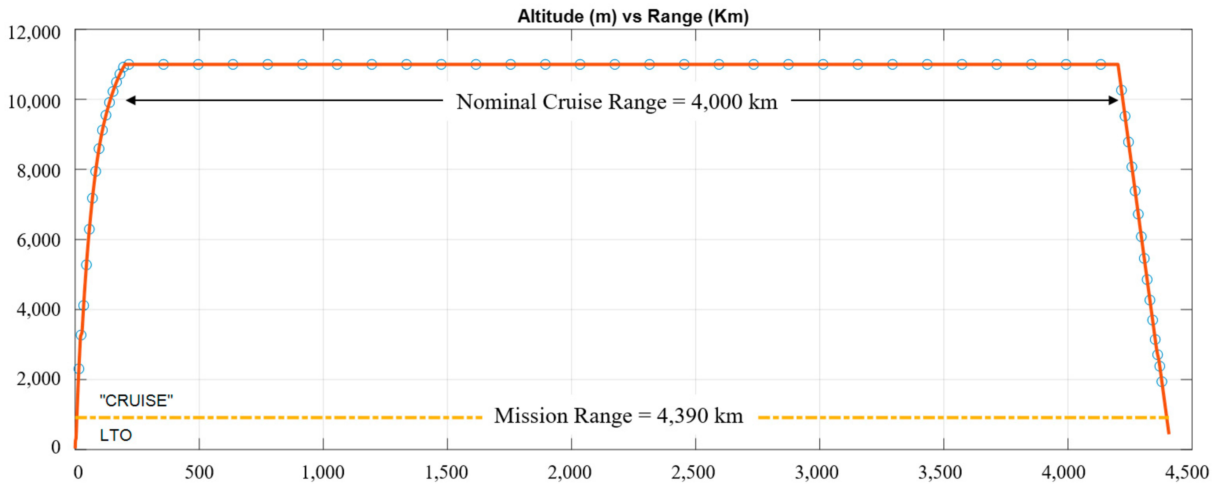
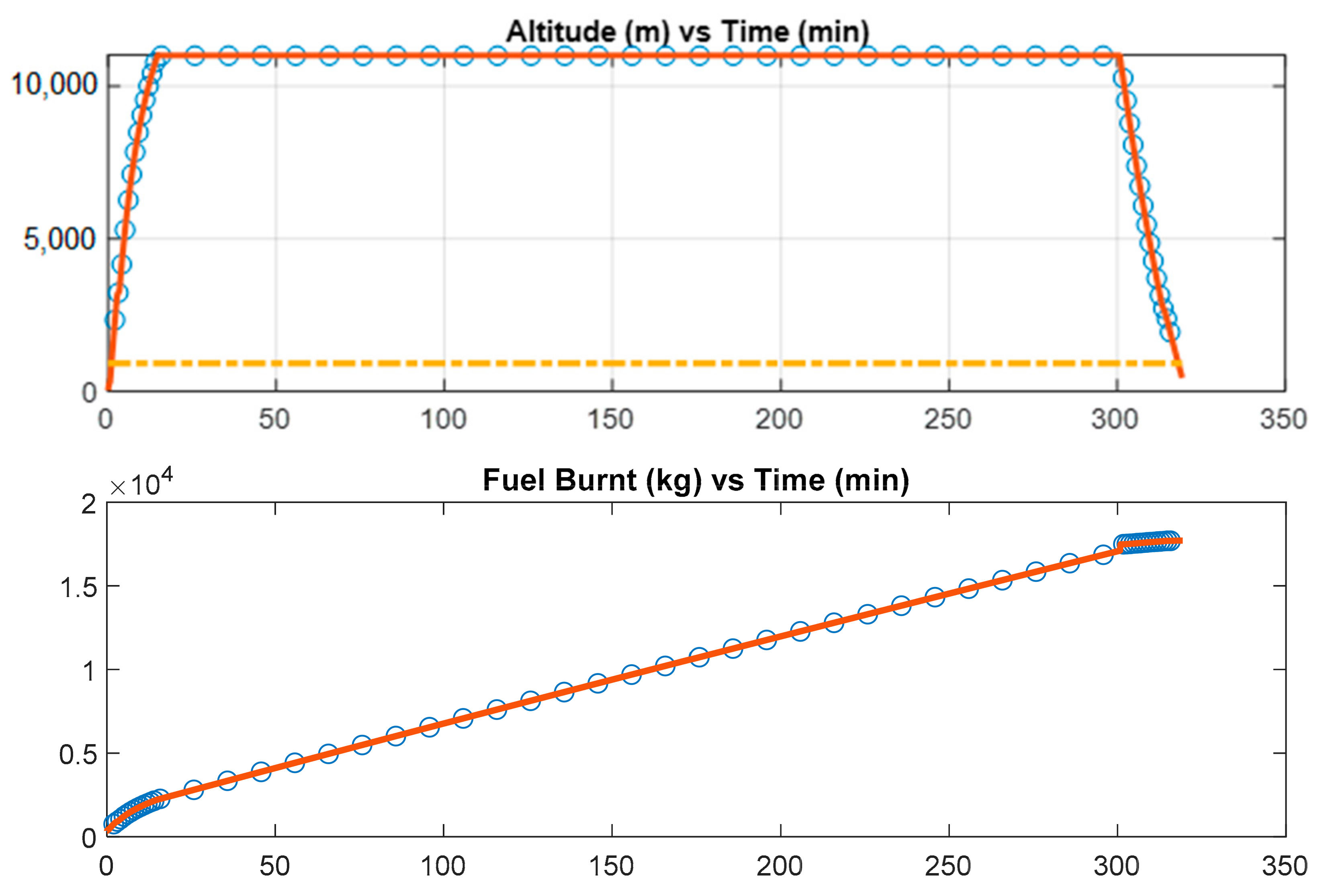
- Definition of the “CRUISE” mission profile as a set of pairs duration-altitude (t,h)i for an arbitrary number of flight phases indicated by the subscript i (see Figure 5);
- 2.
- Evaluation of required engine thrust and fuel flow values at defined flight phases.
- 3.
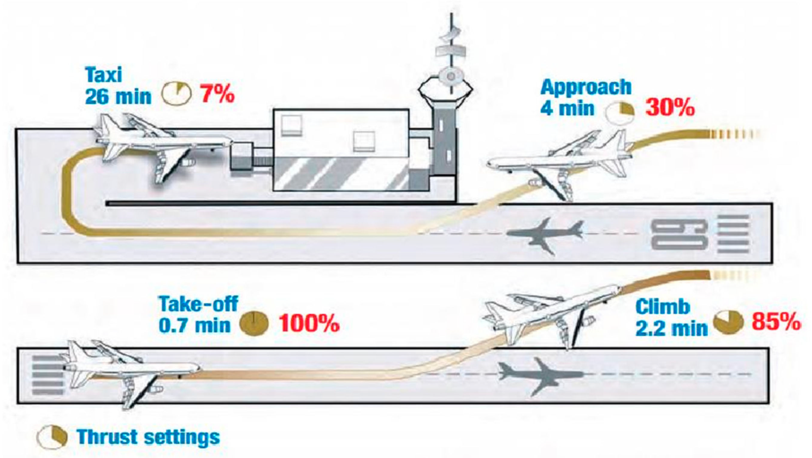
- Definition of LTO emission indices (EI) for aircraft engine, referring to datasets as those available from the ICAO Engine Emissions Databank [62].
- 4.
- Estimation of HC, CO, and NOx emission along the “CRUISE” phase. Since ICAO Engine Emissions data are obtained from certification tests performed at ground level, a correction procedure is needed to take into account altitude effects. The procedure adopted, developed by Boeing, is known as “Fuel Flow Method 2” (FFM2, [9] and aims to correct the emission on the basis of air pressure, temperature and humidity at the given altitude values. Once the corrected emission indices (EI) are evaluated, the emissions from “CRUISE” phase (S) are calculated as follows:where n is the number of segments in which “CRUISE” phase is divided.
- 5.
- Evaluation of hydrocarbons, carbon monoxide and nitrogen oxides emissions during LTO phases multiplying the quantities indicated in the ICAO dataset by the number of engines.
- 6.
- Estimation of total HC, CO, and NOx emissions as sum of “cruise” and LTO contributions.
- (1)
- Interpolating the data of a subset of engines of the ICAO databank, assuming the PrP required maximum thrust (or “rated output”) as input value.
- (2)
2.4. Impact Assessment Method
3. Results
3.1. Fuel Consumption and Emissions
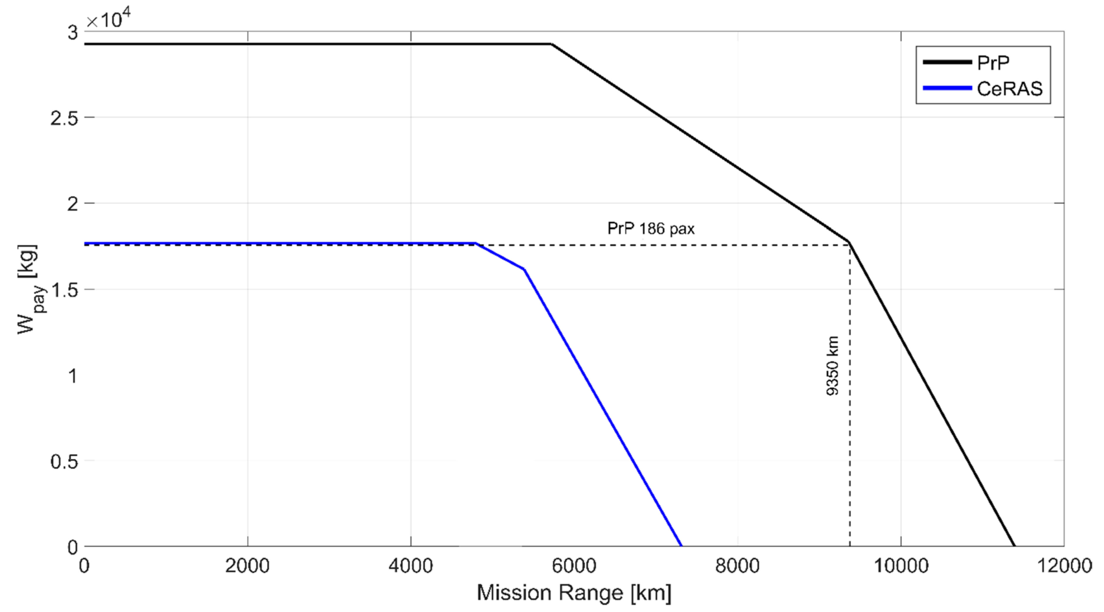
- The higher aerodynamic efficiency of the PrP combined with the higher payload capability, result in a reduction of fuel consumption per pax-km close to 20%, which does not depend on the engine EI estimation approach;
- CO2, H2O and SO2 emissions mainly depend on the “CRUISE” fuel demand. Hence, the fuel saving achievable by the higher aerodynamic performance of the PrP is reflected also on emissions, with small differences depending on the approach adopted to estimate engine EI approach;
- the PrP has lower HC and CO emissions compared to CERAS, although CO is significantly sensitive to engine EI estimation approach;
- NOx emissions variations are less significant and more affected by engine EI estimation approach, as shown by Table 4;
- BC emissions increase although sensitivity to engine EI approach is significant.
- In total, a ~20% reduction of fuel consumption, CO2 and SO2 per passenger-kilometre;
- More than 15% reduction in HC emitted per passenger-kilometre;
- Reduced CO emission per passenger-kilometre;
- Increased emission of Black Carbon (BC).
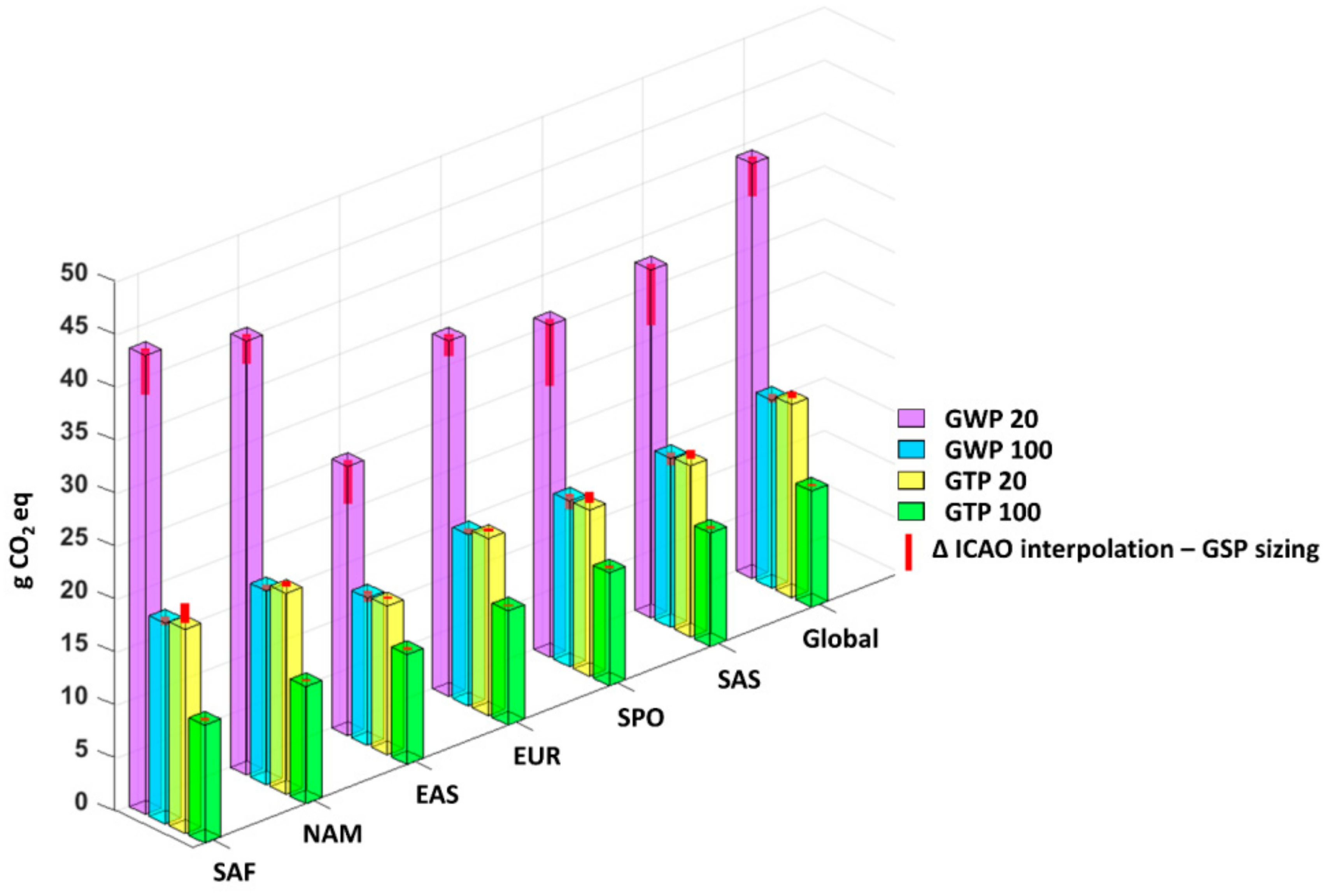
3.2. Impact Assessment of PrandtlPlane Emissions
4. Discussion and Recommendations
4.1. Emission Data and Estimation
4.2. Impact Assessment: Towards a Holistic Approach
4.3. Impact Reduction and Mitigation
4.4. Mass Production: Challenges
5. Conclusions
Supplementary Materials
Author Contributions
Funding
Institutional Review Board Statement
Informed Consent Statement
Data Availability Statement
Conflicts of Interest
Abbreviations
| AFR | air-to-fuel mass ratio |
| BC | black carbon |
| CFD | Computational Fluid Dynamics |
| EI | emission index |
| GTP | Global Temperature Potential |
| GWP | Global Warming Potential |
| HC | hydrocarbons |
| ICAO | International Civil Aviation Organization |
| LCA | Life Cycle Assessment |
| LTO | landing and takeoff |
| PRP | PrandtlPlane |
| RFI | Radiative Forcing Index |
References
- IPCC. Special Report: Global Warming of 1.5 °C. 2018. Available online: https://www.ipcc.ch/sr15/ (accessed on 16 May 2020).
- ICAO. 2019 Environmental Report. Available online: https://www.icao.int/environmental-protection/Pages/envrep2019.aspx (accessed on 16 May 2020).
- Lee, D.S.; Fahey, D.W.; Skowron, A.; Allen, M.R.; Burkhardt, U.; Chen, Q.; Doherty, S.J.; Freeman, S.; Forster, P.M.; Fuglestvedt, J.; et al. The contribution of global aviation to anthropogenic climate forcing for 2000 to 2018. Atmos. Environ. 2021, 244, 117834. [Google Scholar] [CrossRef]
- ICAO. Annual Report of the Council. 2018. Available online: https://www.icao.int/annual-report-2018/Pages/default.aspx (accessed on 16 May 2020).
- ICAO. Annual Report of the Council. 2014. Available online: https://www.icao.int/annual-report-2014/Pages/default.aspx (accessed on 16 May 2020).
- ICAO. Long Term Traffic Forecasts—Passengers and Cargo; ICAO: Quebec, QC, Canada, 2018. [Google Scholar]
- IPCC. Aviation and the Global Atmosphere; Cambridge University Press: Cambridge, UK, 1999. [Google Scholar]
- IPCC. Good Practice Guidance and Uncertainty Management in National Greenhouse Gas Inventories. 2000. Available online: https://www.ipcc-nggip.iges.or.jp/public/gp/english/ (accessed on 9 March 2020).
- Schaefer, M.; Bartosch, S. Overview on Fuel Flow Correlation Methods for the Calculation of NOx, CO and HC Emissions and Their Implementation into Aircraft Performance Software; Report Number: IB-325-11-13; Institut für Antriebstechnik: Köln, Germany, 2013. [Google Scholar]
- Penner, J. Carbonaceous Aerosols Influencing Atmospheric Radiation: Black and Organic Carbon; Lawrence Livermore National Lab.: Livermore, CA, USA, 1994.
- Dessens, O.; Köhler, M.O.; Rogers, H.L.; Jones, R.L.; Pyle, J.A. Aviation and climate change. Transp. Policy 2014, 34, 14–20. [Google Scholar] [CrossRef] [Green Version]
- Jungbluth, N.; Meili, C. Recommendations for calculation of the global warming potential of aviation including the radiative forcing index. Int. J. Life Cycle Assess. 2019, 24, 404–411. [Google Scholar] [CrossRef]
- Azar, C.; Johansson, D.J.A. Valuing the non-CO2 climate impacts of aviation. Clim. Chang. 2012, 111, 559–579. [Google Scholar] [CrossRef] [Green Version]
- Grewe, V.; Dahlmann, K.; Flink, J.; Frömming, C.; Ghosh, R.; Gierens, K.; Heller, R.; Hendricks, J.; Jöckel, P.; Kaufmann, S.; et al. Mitigating the Climate Impact from Aviation: Achievements and Results of the DLR WeCare Project. Aerospace 2017, 4, 34. [Google Scholar] [CrossRef]
- Scheelhaase, J.D.; Dahlmann, K.; Jung, M.; Keimel, H.; Nieße, H.; Sausen, R.; Schaefer, M.; Wolters, F. How to best address aviation’s full climate impact from an economic policy point of view?—Main results from AviClim research project. Transp. Res. Part D Transp. Environ. 2016, 45, 112–125. [Google Scholar] [CrossRef] [Green Version]
- Green, J.E. Air Travel—Greener by Design: Mitigating the Environmental Impact of Aviation: Opportunities and Priorities. Aeronaut. J. 2005, 109, 361–418. [Google Scholar]
- Creemers, W.; Slingerland, R. Impact of Intermediate Stops on Long-Range Jet-Transport Design. In Proceedings of the 7th AIAA ATIO Conf, 2nd CEIAT Int’l Conf on Innov and Integr in Aero Sciences, 17th LTA Systems Tech Conf; followed by 2nd TEOS Forum, Belfast, Northern Ireland, 18–20 September 2007. [Google Scholar]
- Poll, D.I.A. On the effect of stage length on the efficiency of air transport. Aeronaut. J. 2011, 115, 273–283. [Google Scholar] [CrossRef]
- Sausen, R.; Nodorp, D.; Land, C. Towards an optimal flight routing with respect to minimal environmental impact. In Impact of Emissions from Aircraft and Spacecraft upon the Atmosphere; Schumann, U., Wurzel, D., Eds.; DLR: Cologne, Germany, 1994; pp. 473–478. [Google Scholar]
- Mannstein, H.; Spichtinger, P.; Gierens, K. A note on how to avoid contrail cirrus. Transp. Res. Part D Transp. Environ. 2005, 10, 421–426. [Google Scholar] [CrossRef]
- Grewe, V.; Champougny, T.; Matthes, S.; Frömming, C.; Brinkop, S.; Søvde, O.A.; Irvine, E.A.; Halscheidt, L. Reduction of the air traffic’s contribution to climate change: A REACT4C case study. Atmos. Environ. 2014, 94, 616–625. [Google Scholar] [CrossRef] [Green Version]
- Lührs, B.; Linke, F.; Gollnick, V. Erweiterung eines Trajektorienrechners zur Nutzung Meteorologischer Daten für die Optimierung von Flugzeugtrajektorien; Deutsche Gesellschaft für Luft- und Raumfahrt (DGLR): Hamburg, Germany, 2014. [Google Scholar]
- Kyprianidis, K.G. Future Aero Engine Designs: An Evolving Vision. In Advances in Gas Turbine Technology; InTech: Vienna, Austria, 2011; pp. 3–24. [Google Scholar]
- Kyprianidis, K.G.; Dahlquist, E. On the trade-off between aviation NOx and energy efficiency. Appl. Energy 2017, 185, 1506–1516. [Google Scholar] [CrossRef]
- Papadopoulos, T.; Pilidis, P. Introduction of Intercooling in a High Bypass jet Engine; American Society of Mechanical Engineers: New York, NY, USA, 2000. [Google Scholar]
- Rolt, A.M.; Kyprianidis, K.G. Assessment of new aero engine core concepts and technologies in the EU framework 6 NEWAC programme. In Proceedings of the ICAS 2010 Congress Proceedings, Nice, France, 19–24 September 2010. [Google Scholar]
- Xu, L.; Grönstedt, T. Design and Analysis of an Intercooled Turbofan Engine. J. Eng. Gas Turbines Power 2010, 132. [Google Scholar] [CrossRef]
- Da Alves, M.A.; de Franca-Mendes-Carneiro, H.F.; Barbosa, J.R.; Travieso, L.E.; Pilidis, P.; Ramsden, K.W. An insight on intercooling and reheat gas turbine cycles. Proc. Inst. Mech. Eng. Part A J. Power Energy 2001, 215, 163–171. [Google Scholar] [CrossRef]
- Pellischek, G.; Kumpf, B. Compact heat exchanger technology for aero engines. In Proceedings of the 10th Symposium on Air Breathing Engines, Nottingham, UK, 1–6 September 1991. [Google Scholar]
- Xu, L.; Kyprianidis, K.G.; Grönstedt, T.U.J. Optimization Study of an Intercooled Recuperated Aero-Engine. J. Propuls. Power 2013, 29, 424–432. [Google Scholar] [CrossRef]
- McDonald, C.F.; Massardo, A.F.; Rodgers, C.; Stone, A. Recuperated gas turbine aeroengines. Part III: Engine concepts for reduced emissions, lower fuel consumption, and noise abatement. Aircr. Eng. Aerosp. Technol. 2008, 80, 408–426. [Google Scholar] [CrossRef]
- Rosskopf, M.; Lehner, S.; Gollnick, V. Economic–environmental trade-offs in long-term airline fleet planning. J. Air Transp. Manag. 2014, 34, 109–115. [Google Scholar] [CrossRef]
- European Commission. Flightpath 2050: Europe’s Vision for Aviation; European Commission: Brussels, Belgium, 2011. [Google Scholar]
- Apffelstaedt, A.; Langhans, S.; Gollnick, V. Identifying carbon dioxide reducing aircraft technologies and estimating their impact on global CO2 emissions. In Proceedings of the Deutscher Luft-und Raumfahrtkongress, Aachen, Germany, 8–10 September 2009. [Google Scholar]
- NACA. Induced Drag of Multiplanes; Technical Note 182, NACA: Washington, DC, USA, 1924. [Google Scholar]
- Frediani, A.; Montanari, G. Best wing system: An exact solution of the Prandtl’s problem. In Variational Analysis and Aerospace Engineering; Springer: New York, NY, USA, 2009; pp. 183–211. [Google Scholar]
- Frediani, A.; Cipolla, V.; Rizzo, E. The PrandtlPlane Configuration: Overview on Possible Applications to Civil Aviation. In Variational Analysis and Aerospace Engineering: Mathematical Challenges for Aerospace Design; Springer: New York, NY, USA, 2012; pp. 179–210. [Google Scholar]
- Frediani, A.; Cipolla, V.; Oliviero, F. Design of a prototype of light amphibious PrandtlPlane. In Proceedings of the 56th AIAA/ASCE/AHS/ASC Structures, Structural Dynamics, and Materials Conference, Kissimmee, FL, USA, 5–9 January 2015. [Google Scholar] [CrossRef]
- Dales, J.H. Pollution, Property & Prices: An Essay in Policy-Making and Economics; University of Toronto Press: Toronto, ON, Canada, 1968. [Google Scholar]
- Nordhaus, W. How fast should we graze the global commons. Am. Econ. Rev. 1982, 72, 242–246. [Google Scholar]
- Scheelhaase, J.D. How to regulate aviation’s full climate impact as intended by the EU council from 2020 onwards. J. Air Transp. Manag. 2019, 75, 68–74. [Google Scholar] [CrossRef]
- European Commission. EU Emissions Trading System (EU ETS). 2020. Available online: https://ec.europa.eu/clima/policies/ets_en (accessed on 5 May 2020).
- Anger, A.; Köhler, J. Including aviation emissions in the EU ETS: Much ado about nothing? A review. Transp. Policy 2010, 17, 38–46. [Google Scholar] [CrossRef]
- Council of the European Union. Directive EU 2008/101/EC; Council of the European Union: Brussels, Belgium, 2008.
- Council of the European Union. Directive 2009/29/EC; Council of the European Union: Brussels, Belgium, 2009.
- Council of the European Union. COM/2017/054 final; Council of the European Union: Brussels, Belgium, 2017.
- IPCC. Climate Change. The IPCC Impacts Assessment; IPCC: Paris, France, 1990. [Google Scholar]
- Shine, K.P.; Fuglestvedt, J.S.; Hailemariam, K.; Stuber, N. Alternatives to the Global Warming Potential for Comparing Climate Impacts of Emissions of Greenhouse Gases. Clim. Chang. 2005, 68, 281–302. [Google Scholar] [CrossRef] [Green Version]
- IPCC. Climate Change 2013: The Physical Science Basis. Contribution of Working Group I to the Fifth Assessment Report of the Intergovernmental Panel on Climate Change; Cambridge University Press: Cambridge, UK; New York, NY, USA, 2013. [Google Scholar]
- Solomon, S.; Manning, M.; Marquis, M.; Qin, D. Climate Change 2007: The Physical Science Basis. Contribution of Working Group I to the Fourth Assessment Report of the Intergovernmental Panel on Climate Change (IPCC); Cambridge University Press: Cambridge, UK; New York, NY, USA, 2007. [Google Scholar]
- Lee, D.S.; Fahey, D.W.; Forster, P.M.; Newton, P.J.; Wit, R.C.; Lim, L.L.; Owen, B.; Sausen, R. Aviation and global climate change in the 21st century. Atmos. Environ. 2009, 43, 3520–3537. [Google Scholar] [CrossRef] [Green Version]
- Lee, D.S.; Pitari, G.; Grewe, V.; Gierens, K.; Penner, J.E.; Petzold, A.; Prather, M.J.; Schumann, U.; Bais, A.; Berntsen, T.; et al. Transport impacts on atmosphere and climate: Aviation. Atmos. Environ. 2010, 44, 4678–4734. [Google Scholar] [CrossRef] [Green Version]
- Peters, G.P.; Aamaas, B.; Lund, M.T.; Solli, C.; Fuglestvedt, J.S. Alternative ‘Global Warming’ Metrics in Life Cycle Assessment: A Case Study with Existing Transportation Data. Environ. Sci. Technol. 2011, 45, 8633–8641. [Google Scholar] [CrossRef] [PubMed]
- Kollmuss, A.; Crimmins, A. Carbon Offsetting & Air Travel, Part 2: Non-CO2 Emissions Calculations, Stockholm. 2009. Available online: www.co2offsetresearch.org/PDF/SEI_Air_Travel_Emissions_Paper2_June_09.pdf (accessed on 2 March 2020).
- UBA. Klimawirksamkeit des Flugverkehrs: Aktueller Wissenschaftlicher Kenntnisstand Über Die Effekte des Flugverkehrs. Dessau, Germany. 2012. Available online: www.umweltbundesamt.de/klimaschutz/publikationen/klimawirksamkeit_des_flugverkehrs.pdf (accessed on 2 March 2020).
- Abrahamson, J.P.; Zelina, J.; Andac, M.G.; Wal, R.L.V. Predictive Model Development for Aviation Black Carbon Mass Emissions from Alternative and Conventional Fuels at Ground and Cruise. Environ. Sci. Technol. 2016, 50, 12048–12055. [Google Scholar] [CrossRef] [PubMed]
- Köhler, M.O.; Rädel, G.; Shine, K.P.; Rogers, H.L.; Pyle, J.A. Latitudinal variation of the effect of aviation NOx emissions on atmospheric ozone and methane and related climate metrics. Atmos. Environ. 2013, 64, 1–9. [Google Scholar] [CrossRef]
- Lund, M.T.; Aamaas, B.; Berntsen, T.; Bock, L.; Burkhardt, U.; Fuglestvedt, J.S.; Shine, K.P. Emission metrics for quantifying regional climate impacts of aviation. Earth Syst. Dyn. 2017, 8, 547–563. [Google Scholar] [CrossRef] [Green Version]
- PARSIFAL Project 2017–2020, Grant Agreement n. 723149. 2020. Available online: www.parsifalproject.eu (accessed on 4 July 2020).
- CERAS. CeRAS-CSR01: Short Range Reference Aircraft. 2015. Available online: http://ceras.ilr.rwth-aachen.de/trac/wiki/CeRAS/AircraftDesigns/CSR01 (accessed on 4 July 2020).
- ICAO. Airport Air Quality Manual; ICAO: Quebec, QC, Canada, 2011. [Google Scholar]
- ICAO. ICAO Aircraft Engine Emissions Databank. 2019. Available online: https://www.easa.europa.eu/easa-and-you/environment/icao-aircraft-engine-emissions-databank (accessed on 4 July 2020).
- Cipolla, V.; Frediani, A.; Salem, K.A.; Scardaoni, M.P.; Nuti, A.; Binante, V. Conceptual design of a box-wing aircraft for the air transport of the future. In Proceedings of the 2018 AIAA Aviation Technology, Integration, and Operations Conference, Atlanta, GA, USA, 25–29 June 2018. [Google Scholar] [CrossRef]
- Gierens, K.; Dilger, F. A climatology of formation conditions for aerodynamic contrails. Atmos. Chem. Phys. 2013, 13, 10847–10857. [Google Scholar] [CrossRef] [Green Version]
- Stettler, M.E.J.; Boies, A.M.; Petzold, A.; Barrett, S.R.H. Global civil aviation black carbon emissions. Environ. Sci. Technol. 2013, 47, 10397–10404. [Google Scholar] [CrossRef]
- Netherlands Aerospace Centre (NLR). Gas Turbine Simulation Program (GSP). 2020. Available online: www.gspteam.com (accessed on 4 July 2020).
- PARSIFAL Project Consortium. Definition of the Propulsion System for the PrandtlPlane and Steady State Performance Analysis; PARSIFAL Project Deliverable D7.1; European Commission: Luxembourg, 2020. [Google Scholar]
- Cipolla, V.; Salem, K.A.; Scardaoni, M.P.; Binante, V. Preliminary design and performance analysis of a box-wing transport aircraft. In Proceedings of the AIAA Scitech 2020 Forum, Orlando, FL, USA, 6–10 January 2020. [Google Scholar] [CrossRef]
- Joos, F.; Roth, R.; Fuglestvedt, J.S.; Peters, G.P.; Enting, I.G.; Bloh, W.V.; Brovkin, V.; Burke, E.J.; Eby, M.; Edwards, N.R.; et al. Carbon dioxide and climate impulse response functions for the computation of greenhouse gas metrics: A multi-model analysis. Atmos. Chem. Phys. 2013, 13, 2793–2825. [Google Scholar] [CrossRef] [Green Version]
- Samset, B.H.; Myhre, G. Vertical dependence of black carbon, sulphate and biomass burning aerosol radiative forcing. Geophys. Res. Lett. 2011, 38. [Google Scholar] [CrossRef] [Green Version]
- Myhre, G.; Karlsdóttir, S.; Isaksen, I.S.A.; Stordal, F. Radiative forcing due to changes in tropospheric ozone in the period 1980 to 1996. J. Geophys. Res. Atmos. 2000, 105, 28935–28942. [Google Scholar] [CrossRef] [Green Version]
- Holmes, C.D.; Prather, M.J.; Søvde, O.A.; Myhre, G. Future methane, hydroxyl, and their uncertainties: Key climate and emission parameters for future predictions. Atmos. Chem. Phys. 2013, 13, 285–302. [Google Scholar] [CrossRef] [Green Version]
- Wild, O.; Prather, M.J.; Akimoto, H. Indirect long-term global radiative cooling from NO x Emissions. Geophys. Res. Lett. 2001, 28, 1719–1722. [Google Scholar] [CrossRef] [Green Version]
- Myhre, G.; Nilsen, J.S.; Gulstad, L.; Shine, K.P.; Rognerud, B.; Isaksen, I.S.A. Radiative forcing due to stratospheric water vapour from CH4 oxidation. Geophys. Res. Lett. 2007, 34, L01807. [Google Scholar] [CrossRef] [Green Version]
- Bock, L.; Burkhardt, U. The temporal evolution of a long-lived contrail cirrus cluster: Simulations with a global climate model. J. Geophys. Res. Atmos. 2016, 121, 3548–3565. [Google Scholar] [CrossRef] [Green Version]
- Bock, L.; Burkhardt, U. Reassessing properties and radiative forcing of contrail cirrus using a climate model. J. Geophys. Res. Atmos. 2016, 121, 9717–9736. [Google Scholar] [CrossRef] [Green Version]
- Burkhardt, U.; Kärcher, B. Global radiative forcing from contrail cirrus. Nat. Clim. Chang. 2011, 1, 54–58. [Google Scholar] [CrossRef] [Green Version]
- Jaeglé, L.; Jacob, D.J.; Wang, Y.; Weinheimer, A.J.; Ridley, B.A.; Campos, T.L.; Sachse, G.W.; Hagen, D.E. Sources and chemistry of NO x in the upper troposphere over the United States. Geophys. Res. Lett. 1998, 25, 1705–1708. [Google Scholar] [CrossRef] [Green Version]
- Peck, J.; Oluwole, O.O.; Wong, H.-W.; Miake-Lye, R.C. An algorithm to estimate aircraft cruise black carbon emissions for use in developing a cruise emissions inventory. J. Air Waste Manage. Assoc. 2013, 63, 367–375. [Google Scholar] [CrossRef] [Green Version]
- Lohmann, U.; Feichter, J. Global indirect aerosol effects: A review. Atmos. Chem. Phys. 2005, 5, 715–737. [Google Scholar] [CrossRef] [Green Version]
- Haywood, J.M.; Shine, K.P. The effect of anthropogenic sulfate and soot aerosol on the clear sky planetary radiation budget. Geophys. Res. Lett. 1995, 22, 603–606. [Google Scholar] [CrossRef]
- Kärcher, B.; Peter, T.; Biermann, U.M.; Schumann, U. The Initial Composition of Jet Condensation Trails. J. Atmos. Sci. 1996, 53, 3066–3083. [Google Scholar] [CrossRef]
- Heymsfield, A.J.; Lawson, R.P.; Sachse, G.W. Growth of ice crystals in a precipitating contrail. Geophys. Res. Lett. 1998, 25, 1335–1338. [Google Scholar] [CrossRef]
- Righi, M.; Hendricks, J.; Sausen, R. The global impact of the transport sectors on atmospheric aerosol: Simulations for year 2000 emissions. Atmos. Chem. Phys. 2013, 13, 9939–9970. [Google Scholar] [CrossRef] [Green Version]
- Shindell, D.T.; Faluvegi, G.; Koch, D.M.; Schmidt, G.A.; Unger, N.; Bauer, S.E. Improved Attribution of Climate Forcing to Emissions. Science 2009, 326, 716–718. [Google Scholar] [CrossRef] [Green Version]
- Grewe, V.; Stenke, A. AirClim: An efficient tool for climate evaluation of aircraft technology. Atmos. Chem. Phys. 2008, 8, 4621–4639. [Google Scholar] [CrossRef] [Green Version]
- Köhler, M.O.; Rädel, G.; Dessens, O.; Shine, K.P.; Rogers, H.L.; Wild, O.; Pyle, J.A. Impact of perturbations to nitrogen oxide emissions from global aviation. J. Geophys. Res. 2008, 113, D11305. [Google Scholar] [CrossRef] [Green Version]
- Stevenson, D.S. Radiative forcing from aircraft NO x emissions: Mechanisms and seasonal dependence. J. Geophys. Res. 2004, 109, D17307. [Google Scholar] [CrossRef] [Green Version]
- Stevenson, D.S.; Derwent, R.G. Does the location of aircraft nitrogen oxide emissions affect their climate impact? Geophys. Res. Lett. 2009, 36, L17810. [Google Scholar] [CrossRef] [Green Version]
- Sausen, R.; Gierens, K.; Ponater, M.; Schumann, U. A Diagnostic Study of the Global Distribution of Contrails Part I: Present Day Climate ast. Theor. Appl. Climatol. 1998, 61, 127–141. [Google Scholar] [CrossRef] [Green Version]
- Newinger, C.; Burkhardt, U. Sensitivity of contrail cirrus radiative forcing to air traffic scheduling. J. Geophys. Res. Atmos. 2012, 117. [Google Scholar] [CrossRef] [Green Version]
- Vázquez-Navarro, M.; Mannstein, H.; Kox, S. Contrail life cycle and properties from 1 year of MSG/SEVIRI rapid-scan images. Atmos. Chem. Phys. 2015, 15, 8739–8749. [Google Scholar] [CrossRef] [Green Version]
- Meerkötter, R.; Schumann, U.; Doelling, D.R.; Minnis, P.; Nakajima, T.; Tsushima, Y. Radiative forcing by contrails. Ann. Geophys. 1999, 17, 1080–1094. [Google Scholar] [CrossRef]
- Irvine, E.A.; Shine, K.P. Ice supersaturation and the potential for contrail formation in a changing climate. Earth Syst. Dyn. 2015, 6, 555–568. [Google Scholar] [CrossRef] [Green Version]
- ICAO. Airport Air Quality Guidance Manual; ICAO: Montreal, QC, Canada, 2011. [Google Scholar]
- Döpelheuer, A.; Lecht, M. Influence of engine performance on emission characteristics. In Gas Turbine Engine Combustion, Emissions and Alternative Fuels; CRC Press: Boca Raton, FL, USA, 1998. [Google Scholar]
- Speth, R.L.; Rojo, C.; Malina, R.; Barrett, S.R.H. Black carbon emissions reductions from combustion of alternative jet fuels. Atmos. Environ. 2015, 105, 37–42. [Google Scholar] [CrossRef]
- Schumann, U. AERONOX/The Impact of NOx Emissions from Aircraft Upon the Atmosphere at Flight Altitudes 8–15 km; Final Report to the Commission of European Communities; Institute of Atmospheric Physics: Oberpfaffenhofen, Germany, 1995. [Google Scholar]
- Norman, P.D.; Lister, D.H.; Lecht, M.; Madden, P.; Park, K.; Penanhoat, O. Development of the Technical Basis for a New Emissions Parameter Covering the Whole AIRcraft Operation: NEPAIR; Final Technical Report; EU Publications Office: Luxembourg, 2003. [Google Scholar]
- Deidewig, F.; Döpelheuer, A.; Lecht, M. Methods to Assess Aircraft Engine Emissions in Flight. ICAS Proc. 1996, 20, 131–141. [Google Scholar]
- Baughcum, S.L.; Tritz, T.G.; Henderson, S.C.; Pickett, D.C. Scheduled Civil Analysis, Aircraft Emission Inventories for 1992: Database Development and NASA Contractor Report 4700; NASA: Washington, DC, USA, 1996.
- Martin, R.L.; Oncina, C.H.; Zeeben, P.J. A Simplified Method for Estimating Aircraft Engine Emissions. ICAO/CAEP/Working Group 3, Certification Subgroup, March 1995. Reported as ‘Boeing Method 2’ Fuel Flow Methodology Description in Appendix D of “Scheduled Civil Aircraft Emission Inventories f, 1996. Available online: https://ntrs.nasa.gov/search.jsp?R=19960038445 (accessed on 4 July 2020).
- Masiol, M.; Harrison, R.M. Aircraft engine exhaust emissions and other airport-related contributions to ambient air pollution: A review. Atmos. Environ. 2014, 95, 409–455. [Google Scholar] [CrossRef] [Green Version]
- Fahey, D.W.; Lee, D.S. Aviation and the Impacts of Climate Change Aviation and Climate Change: A Scientific Perspective. Carbon Clim. Law Rev. 2016, 10, 97–104. [Google Scholar]
- Turgut, E.T.; Cavcar, M.; Usanmaz, O.; Yay, O.D.; Dogeroglu, T.; Armutlu, K. Investigating actual landing and takeoff operations for time-in-mode, fuel and emissions parameters on domestic routes in Turkey. Transp. Res. Part D Transp. Environ. 2017, 53, 249–262. [Google Scholar] [CrossRef]
- Skowron, A.; Lee, D.S.; de León, R.R. The assessment of the impact of aviation NOx on ozone and other radiative forcing responses—The importance of representing cruise altitudes accurately. Atmos. Environ. 2013, 74, 159–168. [Google Scholar] [CrossRef] [Green Version]
- Myhre, G.; Shine, K.P.; Rädel, G.; Gauss, M.; Isaksen, I.S.A.; Tang, Q.; Prather, M.J.; Williams, J.E.; van Velthoven, P.; Dessens, O.; et al. Radiative forcing due to changes in ozone and methane caused by the transport sector. Atmos. Environ. 2011, 45, 387–394. [Google Scholar] [CrossRef] [Green Version]
- Fuglestvedt, J.S.; Shine, K.P.; Berntsen, T.; Cook, J.; Lee, D.S.; Stenke, A.; Skeie, R.B.; Velders, G.J.M.; Waitz, I.A. Transport impacts on atmosphere and climate: Metrics. Atmos. Environ. 2010, 44, 4648–4677. [Google Scholar] [CrossRef] [Green Version]
- Schulz, M.; Textor, C.; Kinne, S.; Balkanski, Y.; Bauer, S.; Berntsen, T.; Boucher, O.; Dentener, F.; Guibert, S.; Isaksen, I.S.A.; et al. Radiative forcing by aerosols as derived from the AeroCom present-day and pre-industrial simulations. Atmos. Chem. Phys. 2006, 6, 5225–5246. [Google Scholar] [CrossRef] [Green Version]
- Frediani, A.; Cipolla, V.; Salem, K.A.; Binante, V.; Scardaoni, M.P. Conceptual design of PrandtlPlane civil transport aircraft. Proc. Inst. Mech. Eng. Part G J. Aerosp. Eng. 2019. [Google Scholar] [CrossRef] [Green Version]
- PARSIFAL Project Consortium. PrandtlPlane Performance Analysis and Scaling Procedures, PARSIFAL Project Deliverable, D 3.4; European Commission: Luxembourg, 2020; CORDIS Website; Available online: https://cordis.europa.eu/project/id/723149/results (accessed on 4 March 2021).
- Carini, M.; Meheut, M.; Kanellopoulos, S.; Cipolla, V.; Salem, K.A. Aerodynamic analysis and optimization of a boxwing architecture for commercial airplanes. In Proceedings of the AIAA Scitech 2020 Forum, Orlando, FL, USA, 6–10 January 2020. [Google Scholar] [CrossRef]
- Frömming, C.; Ponater, M.; Dahlmann, K.; Grewe, V.; Lee, D.S.; Sausen, R. Aviation-induced radiative forcing and surface temperature change in dependency of the emission altitude. J. Geophys. Res. Atmos. 2012, 117. [Google Scholar] [CrossRef] [Green Version]
- Dahlmann, K.; Grewe, V.; Frömming, C.; Burkhardt, U. Can we reliably assess climate mitigation options for air traffic scenarios despite large uncertainties in atmospheric processes? Transp. Res. Part D Transp. Environ. 2016, 46, 40–55. [Google Scholar] [CrossRef] [Green Version]
- Grewe, V.; Dahlmann, K. How ambiguous are climate metrics? And are we prepared to assess and compare the climate impact of new air traffic technologies? Atmos. Environ. 2015, 106, 373–374. [Google Scholar] [CrossRef] [Green Version]
- Faber, J.; Greenwood, D.; Lee, D.; Mann, M.; de Leon, P.M.; Nelissen, D.; Owen, B.; Ralph, M.; Tilston, J.; van Velzen, A.; et al. Lower NOx at Higher Altitudes. Policies to Reduce the Climate Impact of Aviation NOx Emission; CE: Delft, The Netherlands, 2008. [Google Scholar]
- ICAO. ICAO Environmental Report 2010; ICAO: Montreal, QC, Canada, 2010. [Google Scholar]
- Freeman, S.; Lee, D.S.; Lim, L.L.; Skowron, A.; de León, R.R. Trading off Aircraft Fuel Burn and NO x Emissions for Optimal Climate Policy. Environ. Sci. Technol. 2018, 52, 2498–2505. [Google Scholar] [CrossRef] [Green Version]
- de Saint-Exupéry, A. Citadelle; ACT: Moscow, Russia, 1948. [Google Scholar]


| Manufacturer | Engine Identification | B/P Ratio | Rated Thrust Foo (kN) |
|---|---|---|---|
| CFM International | LEAP-1A24/24E1/23 | 11.3 | 106.8 |
| CFM International CFM International | LEAP-1A26/26E1 | 11.1 | 120.6 |
| CFM International | LEAP-1A26CJ | 11.1 | 120.6 |
| CFM International | LEAP-1A29 | 10.7 | 130.3 |
| CFM International | LEAP-1A29CJ | 10.7 | 130.3 |
| CFM International | LEAP-1A35A/33/33B2/32/30 | 10.5 | 143.1 |
| PARSIFAL expected [67] | PrP engine | 11 | 180 |
| Rolls-Royce plc | Trent 1000-H3 | 9.3 | 287.1 |
| Rolls-Royce plc | Trent 1000-AE3 | 9.2 | 310.9 |
| Rolls-Royce plc | Trent 1000-G3 | 9.1 | 323.7 |
| Rolls-Royce plc | Trent 7000-72 | 9 | 327.9 |
| Rolls-Royce plc | Trent 7000-72C | 9 | 327.9 |
| LTO Cycle: “ICAO Interpolation” Approach | Emissions Indices (EI) | |||||
|---|---|---|---|---|---|---|
| Power Setting | Time | Fuel Flow | HC | CO | NOx | |
| Foo [kN] = 180 | % Foo | min | kg s−1 | g kg−1 | g kg−1 | g kg−1 |
| TAKE-OFF | 100 | 0.7 | 1.332 | 0.023 | 0.301 | 42.372 |
| CLIMB OUT | 85 | 2.2 | 1.097 | 0.015 | 0.320 | 23.899 |
| APPROACH | 30 | 4 | 0.369 | 0.030 | 2.026 | 10.330 |
| IDLE | 7 | 26 | 0.148 | 0.203 | 17.134 | 5.047 |
| TOTALS | 33 | 519 | 53 | 4186 | 7907 | |
| LTO cycle: “GSP sizing” approach | Emissions indices (EI) | |||||
| Power setting | Time | Fuel flow | HC | CO | NOx | |
| Foo [kN] = 180 | % Foo | min | Kg s−1 | g kg−1 | g kg−1 | g kg−1 |
| TAKE-OFF | 100 | 0.7 | 1.203 | 0.020 | 0.172 | 36.310 |
| CLIMB OUT | 85 | 2.2 | 0.994 | 0.020 | 0.211 | 21.452 |
| APPROACH | 30 | 4 | 0.375 | 0.031 | 1.167 | 9.102 |
| IDLE | 7 | 26 | 0.139 | 0.128 | 9.384 | 5.498 |
| TOTALS | 33 | 489 | 34 | 2181 | 6662 | |
| Aircraft | Engines (Number = 2) | N. Passengers (Load Factor = 1) | “CRUISE” Range | “CRUISE” Fuel Consumption (kg) | LTO Fuel Consumption (kg) |
|---|---|---|---|---|---|
| CERAS | LEAP 1A-26 | 186 | 4391 | 12,152 | 695 |
| PrP | ICAO int. | 308 | 4343 | 15,889 | 1038 |
| GSP sizing | 978 |
| Case | Fuel | NOx | CO2 | SO2 | BC |
|---|---|---|---|---|---|
| CERAS [g/(pax∙km)] | 15.729 | 0.09321 | 49.62607 | 0.01573 | 0.00026 |
| PrP−ICAO [g/(pax∙km)] | 12.656 | 0.09861 | 39.92833 | 0.01266 | 0.00035 |
| Δ% | −19.5% | +5.8% | −19.5% | −19.5% | +34.2% |
| PrP−GSP [g/(pax∙km)] | 12.609 | 0.09158 | 39.78283 | 0.01261 | 0.00029 |
| Δ% | −19.8% | −1.7% | −19.8% | −19.8% | +11.5% |
| Component | Source Region | CERAS | PRANDTLPLANE | ||||||
|---|---|---|---|---|---|---|---|---|---|
| GWP20 | GWP100 | GTP20 | GTP100 | GWP20 | GWP100 | GTP20 | GTP100 | ||
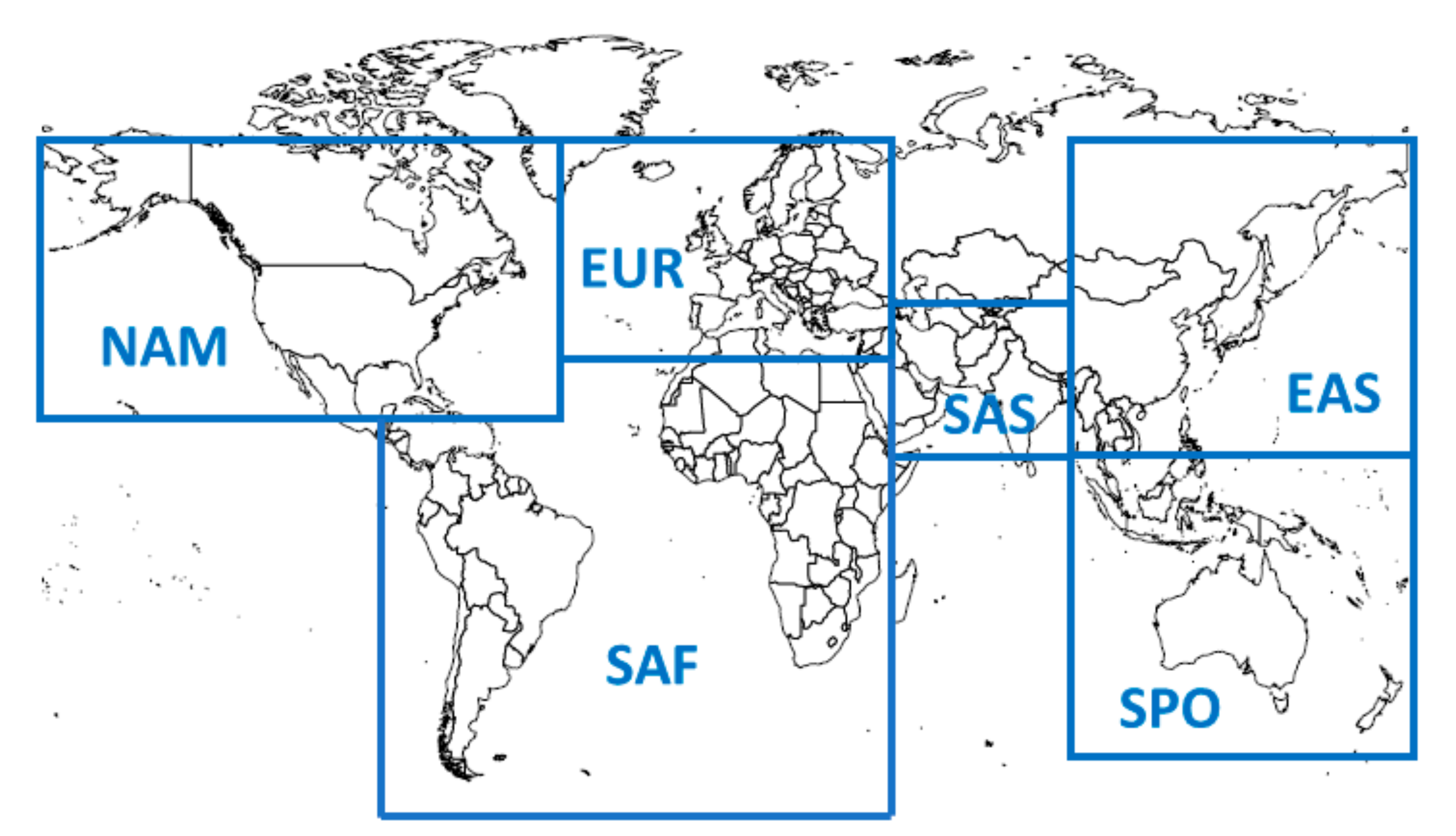
| Contrail cirrus | SAF | 178.65 | 49.13 | 54.09 | 6.95 | 143.22 | 39.38 | 43.36 | 5.57 |
| NAM | 163.77 | 44.66 | 49.63 | 6.45 | 131.28 | 35.80 | 39.78 | 5.17 | |
| EAS | 84.36 | 22.33 | 24.81 | 2.98 | 67.63 | 17.90 | 19.89 | 2.39 | |
| EUR | 124.07 | 33.25 | 37.22 | 4.96 | 99.46 | 26.65 | 29.84 | 3.98 | |
| SPO | 114.14 | 31.26 | 34.74 | 4.47 | 91.50 | 25.06 | 27.85 | 3.58 | |
| SAS | 129.03 | 34.74 | 38.71 | 4.96 | 103.44 | 27.85 | 31.03 | 3.98 | |
| Global | 153.84 | 41.69 | 46.15 | 5.96 | 123.33 | 33.42 | 37.00 | 4.77 | |
| BC | SAF | 1.40 | 0.38 | 0.40 | 0.05 | 1.56 | 0.42 | 0.45 | 0.06 |
| NAM | 0.92 | 0.25 | 0.27 | 0.03 | 1.02 | 0.28 | 0.30 | 0.04 | |
| EAS | 1.08 | 0.29 | 0.31 | 0.04 | 1.20 | 0.33 | 0.35 | 0.04 | |
| EUR | 0.59 | 0.21 | 0.22 | 0.03 | 0.66 | 0.23 | 0.25 | 0.03 | |
| SPO | 1.27 | 0.35 | 0.37 | 0.05 | 1.42 | 0.39 | 0.41 | 0.05 | |
| SAS | 2.13 | 0.58 | 0.62 | 0.08 | 2.37 | 0.65 | 0.69 | 0.09 | |
| Global | 1.01 | 0.27 | 0.29 | 0.04 | 1.12 | 0.30 | 0.33 | 0.04 | |
| SO2 | SAF | −13.10 | −3.57 | −3.81 | −0.49 | −10.50 | −2.86 | −3.05 | −0.39 |
| NAM | −8.65 | −2.36 | −2.50 | −0.33 | −6.94 | −1.89 | −2.00 | −0.26 | |
| EAS | −9.47 | −2.58 | −2.75 | −0.36 | −7.59 | −2.07 | −2.21 | −0.29 | |
| EUR | −5.95 | −1.62 | −1.73 | −0.22 | −4.77 | −1.30 | −1.39 | −0.18 | |
| SPO | −11.73 | −3.19 | −3.40 | −0.44 | −9.41 | −2.56 | −2.72 | −0.35 | |
| SAS | −17.62 | −4.78 | −5.10 | −0.66 | −14.12 | −3.83 | −4.09 | −0.53 | |
| Global | −8.79 | −2.39 | −2.55 | −0.33 | −7.05 | −1.92 | −2.04 | −0.26 | |
| NOx | SAF | 45.11 | 6.52 | −29.45 | 0.58 | 44.33 | 6.41 | −28.94 | 0.57 |
| NAM | 26.10 | 4.47 | −11.74 | 0.47 | 25.64 | 4.40 | −11.54 | 0.46 | |
| EAS | 47.82 | 10.07 | −7.36 | 1.21 | 46.98 | 9.89 | −7.23 | 1.19 | |
| EUR | 19.57 | 3.45 | −8.11 | 0.37 | 19.23 | 3.39 | −7.97 | 0.37 | |
| SPO | 75.13 | 14.82 | −19.11 | 1.77 | 73.81 | 14.56 | −18.77 | 1.74 | |
| SAS | 64.78 | 12.77 | −16.40 | 1.49 | 63.65 | 12.55 | −16.12 | 1.47 | |
| Global | 38.31 | 7.18 | −12.86 | 0.84 | 37.64 | 7.05 | −12.64 | 0.82 | |
| CO2 | SAF | 49.63 | 49.63 | 49.63 | 49.63 | 39.78 | 39.78 | 39.78 | 39.78 |
| NAM | 49.63 | 49.63 | 49.63 | 49.63 | 39.78 | 39.78 | 39.78 | 39.78 | |
| EAS | 49.63 | 49.63 | 49.63 | 49.63 | 39.78 | 39.78 | 39.78 | 39.78 | |
| EUR | 49.63 | 49.63 | 49.63 | 49.63 | 39.78 | 39.78 | 39.78 | 39.78 | |
| SPO | 49.63 | 49.63 | 49.63 | 49.63 | 39.78 | 39.78 | 39.78 | 39.78 | |
| SAS | 49.63 | 49.63 | 49.63 | 49.63 | 39.78 | 39.78 | 39.78 | 39.78 | |
| Global | 49.63 | 49.63 | 49.63 | 49.63 | 39.78 | 39.78 | 39.78 | 39.78 | |
Publisher’s Note: MDPI stays neutral with regard to jurisdictional claims in published maps and institutional affiliations. |
© 2021 by the authors. Licensee MDPI, Basel, Switzerland. This article is an open access article distributed under the terms and conditions of the Creative Commons Attribution (CC BY) license (http://creativecommons.org/licenses/by/4.0/).
Share and Cite
Tasca, A.L.; Cipolla, V.; Abu Salem, K.; Puccini, M. Innovative Box-Wing Aircraft: Emissions and Climate Change. Sustainability 2021, 13, 3282. https://doi.org/10.3390/su13063282
Tasca AL, Cipolla V, Abu Salem K, Puccini M. Innovative Box-Wing Aircraft: Emissions and Climate Change. Sustainability. 2021; 13(6):3282. https://doi.org/10.3390/su13063282
Chicago/Turabian StyleTasca, Andrea Luca, Vittorio Cipolla, Karim Abu Salem, and Monica Puccini. 2021. "Innovative Box-Wing Aircraft: Emissions and Climate Change" Sustainability 13, no. 6: 3282. https://doi.org/10.3390/su13063282