Assessing the Effectiveness of Mitigation Strategies for Flood Risk Reduction in the Segamat River Basin, Malaysia

Abstract

Flooding is a frequent, naturally recurring phenomenon worldwide that can become disastrous if not addressed accordingly. This paper aims to evaluate the impacts of land use change and climate change on flooding in the Segamat River Basin, Johor, Malaysia, with 1D–2D hydrodynamic river modeling, using InfoWorks Integrated Catchment Modeling (ICM). The study involved the development of flood maps for four different scenarios: (1) future land use in 2030; (2) the impacts of climate change; (3) three mitigation strategies comprising detention ponds, rainwater harvesting systems (RWHSs), and permeable pavers; and (4) a combination of these three mitigation strategies. The obtained results show increases in the flood peaks under both the land use change and climate change scenarios. With the anticipated increase in development activities within the vicinity up to 2030, the overall impact of urbanization on the extent of flooding would be rather moderate, as the upper and middle parts of the basin would still be dominated by forests and agricultural activities (approximately 81.13%). In contrast, the potential flood-inundated area is expected to increase from 12.25% to 16.64% under storms of 10-, 50-, 100-, and 1000-year average recurrence intervals (ARI). Interestingly, the simulation results suggest that only the detention pond mitigation strategy has a considerable impact on reducing floods, while the other two mitigation strategies have less flood reduction advantages for this agricultural-based rural basin located in a tropical region.

1. Introduction

Flooding is a common, frequent, naturally recurring global phenomenon that occasionally turns into a destructive disaster. Flooding can be attributed to overbank spills that occur due to inadequate or undersized river channel capacities, lack of maintenance of drainage systems to ensure effectiveness in conveying increases in flood discharges, high channel roughness, siltation, and blockages by floating pollutants such as debris and municipal refuse. In addition, updated knowledge about ever-changing rainfall patterns is also essential, as rainfall is a crucial climatological variable in addressing flood generation and the level of water-related hazards that flooding brings. Numerous studies conducted to detect the changing patterns and amounts of rainfall have been documented based on global [1], regional [2,3], and local scales [4,5]. Studies related to climate change have shown that changes in the rainfall amount, frequency, and intensity substantially intensify flooding, stormwater runoff, and soil erosion [6,7,8,9,10,11].

Currently, flood risk reduction and management programs provide generic options focusing on controlling the source of floods or controlling the pathway and exposure of and vulnerability to floods [12]. Mitigation approaches designed to deal with flood risks have changed over recent years, from primitive approaches such as building houses on higher ground or boats as means of escaping from dangerous areas [13], to engineering approaches such as constructing flood detention ponds and dams, improving river hydraulic capacities, and building flood protection walls and bunds. Generally, engineering approaches, which are achieved by employing structural measures, utilize physical construction that is undertaken to reduce flood levels and the extents of floods. In recent years, much of the flood-related literature has recorded the successful application of rainwater harvesting systems (RWHSs), while the use of permeable or porous pavements related to flood reduction has significantly increased in recent years. For instance, RWHSs can not only reduce flood risks in urban areas [14,15], although they do not eliminate flooding completely, but can also serve as an effective alternative water supply solution by storing rainwater for reuse. The use of these systems also has the added advantages of retaining storm runoff excess from rainfall events with the consequent control of the stormwater flood volume [16,17,18,19]. Permeable pavements are those made with built-in void spaces to facilitate water infiltration into the ground and for air to pass through. Due to the implementation of permeable or porous pavements as an integral part of multifaceted concerns in urban design and in considering the effects of cost–benefit evaluations, permeable or porous pavements are the most radical, rapidly developing, and controversial way of restoring large parts of the urban environment [20]. Therefore, the application of stormwater management systems such as RWHSs and permeable or porous pavements could be among the techniques that are accessible to the community in managing floods and water scarcity [15,21]. With the advancement of technologies, conventional engineering approaches using structural measures are now geared towards an integrated and holistic flood risk management (FRM) approach globally, especially in the European Union [22,23,24], and have been adapted in Asia [25,26]. This involves a combination of management measures, including structural (designed to modify flood characteristics) and non-structural (designed to reduce flood damage and vulnerability through planning and response) measures [25,27,28].

Changes in the water balance that occur due to land use and climate change in tropical countries such as Malaysia not only lead to water shortages during extended dry periods but also increase flood risk because of increased rainfall intensity. In fact, flood incidences in the state of Johor are increasing along the major rivers, which have greatly affected the people who live near or within flood-prone areas. Johor state is Peninsular Malaysia’s largest contributor to agricultural gross domestic product, and its official rate of agricultural productivity is Malaysia’s third highest. The intensity and urbanization levels are higher in the lower river basin than in the upper and middle river basins. In December 2006 and January 2007, a disastrous flood occurred in Johor that affected more than 104,023 people [29] and caused a total loss of USD 369 million [30]. The effects of flooding are felt the most in built-up areas, such as residential and commercial areas within the urban confinement located in the lower river basin, where property damage is higher than in areas with agricultural activities.

River basin variability, including differences in topography, basin size and shape, and watercourses, are among the factors affecting a streamflow; however, the contributing factors of both land use and climate change on flow variations are among the main variables affecting basin hydrology [31,32,33,34]. The Segamat River Basin is a typical tropical, agricultural, rural river basin located in the southern part of Peninsular Malaysia. Several major floods have been experienced in the Segamat River Basin, caused by a series of storm events brought about by the Northeast Monsoon. According to historical flood records, Segamat town was affected the most by the 1969, 1979, 1983, 2007, and 2011 floods. The damage caused by the 2011 flood in Segamat town was estimated at USD 146.2 million [35].

Recently, many flood studies have shifted from small local scales to medium and large basin scales, as well as from exploring a single mitigation strategy to combinations of several mitigation strategies. The literature has shown that the use of a combination of multiple stormwater management practices is more efficient in controlling flooding than the use of a single strategy alone [36,37]. Hence, the current research aims to evaluate the impacts of land use and climate changes, as well as of three mitigation strategies (including detention ponds, RWHSs, and permeable pavers), on floods by utilizing the critical storm duration concept to estimate the extent of the highest possible (maximum) flood for the Segamat River Basin, Malaysia. This aim involves the development of flood maps for four scenarios: (1) land use change impacts; (2) climate change impacts; (3) three mitigation strategies; and (4) a combination of the three mitigation strategies. The use of flood inundation models in current research involves a mixed 1D–2D approach, which has been augmented and successfully applied to large and complex river systems by many researchers (e.g., [38,39,40,41,42]). In particular, the application of 1D–2D flood inundation models in such a large-scale basin provides a compendium as an efficient tool for discharge predictions to quantify the changes in peak flow and the flood inundation response to land use and climate changes, as well as the performances of detention ponds, RWHSs, and permeable paver provisions in this tropical river basin. A similar assessment was performed to assess stormwater management approaches using swales, rain gardens, and other strategies, however this study was applied mainly to small urban catchments [36,37]. However, relatively few studies have examined how stormwater management practices help to reduce urban floods in rural basins, such as the Segamat River Basin. In addition, previous studies performed in the Segamat River Basin have mostly focused on flood simulations and flood risk assessments [43] rather than on analyses of peak discharges for each individual sub-basin or on the performance of mitigation strategies such as RWHSs, detention ponds, and permeable pavers; thus, this study is deemed crucial for evaluating the impacts of nature-based solutions on flooding in rural basins to complement past studies [7,30,35].

2. Materials and Methods

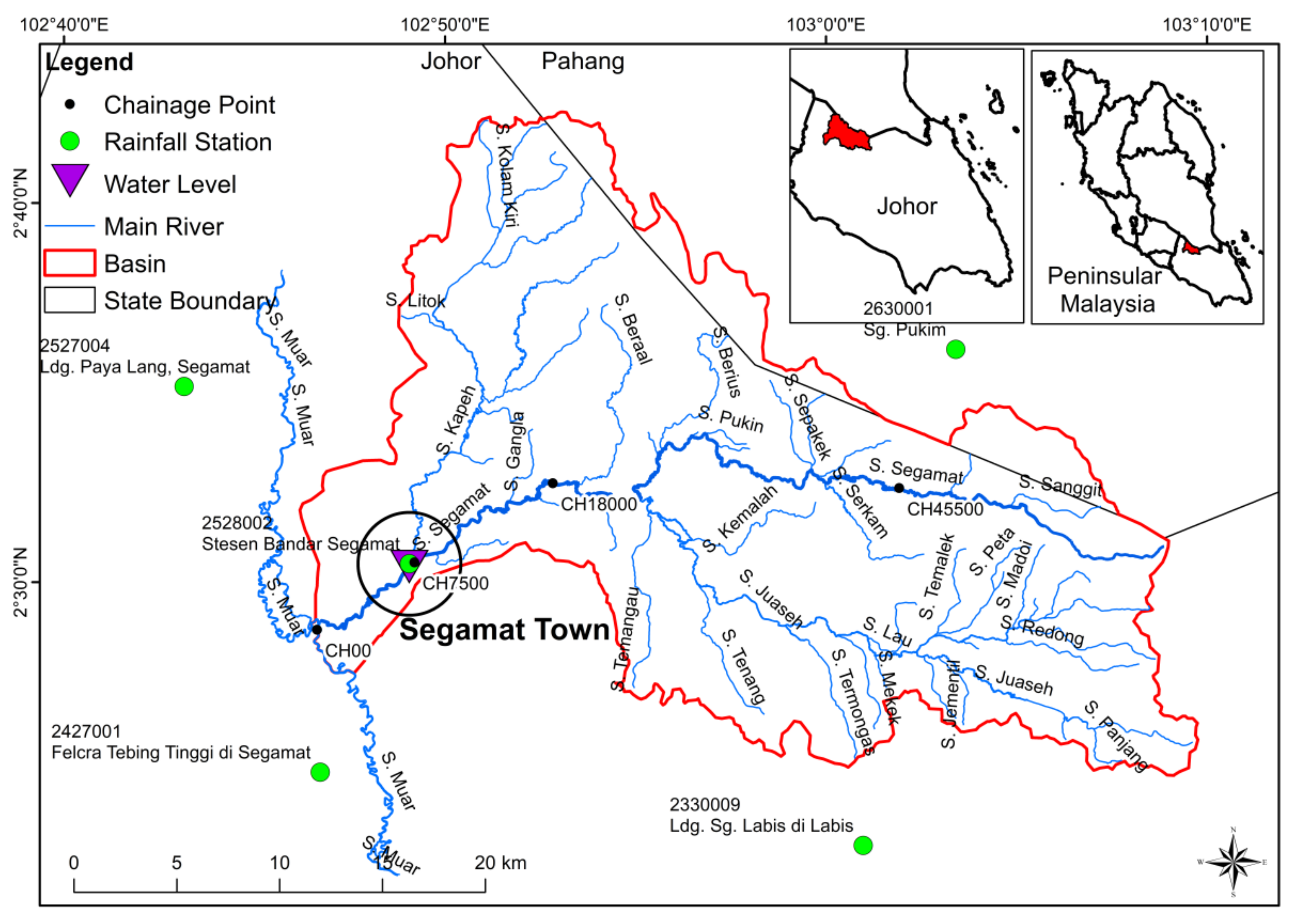
2.1. Study Area

The Segamat River Basin is located between latitudes of 2° 25′ N and 2°42′ N and between longitudes of 102°45’ E and 103°10’ E, covering an area of 701.06 km² (Figure 1). Approximately 70% of the sub-basin is highland with ground elevations up to 1000 m, while the remaining area (30%) consists of hillsides with swampy areas. The Segamat River originates from the eastern projecting mountainous area that holds Mount Besar and joins the Muar River, which flows through Segamat town (Chainage 7500) downstream (Chainage 0). The total length of the Segamat River is approximately 61.8 km, and the river ranges from 9 m to 90 m wide. The annual rainfall varies from approximately 1400 to 2000 mm within the Segamat River Basin. The normal rainy season starts in October, and maximum monthly average rainfall totals are observed in November of a given year to January of the following year at most of the rainfall stations. The mean monthly discharge recorded from 1961 to 2009 was 14 m³/s; this value was recorded at the Segamat River water level monitoring station (Station ID 2528414). However, the mean monthly discharge recorded during most major flood events occurred in November of a given year and January of the following year, which is consistent with the rainy season, while the mean monthly discharge during major flood events was found to rise to 191 m³/s.

Rural development in the Segamat River Basin mainly involves agricultural activities, such as rubber and oil palm plantations, farming, and livestock. Agricultural land accounts for 473.50 km² (67.54%) and dominates all other activities in the Segamat River Basin. In 2017, agricultural land was followed by forests (171.81 km²), developed areas (24.22 km²), transportation areas (16.66 km²), and waterbodies (15.39 km²). Segamat town is located 5.5 km from the river confluence and serves as the center of the state territory and administrative district. However, flooding around the confluence of the Segamat River is severe due to the influence of the backwater from the Muar River, as well as the high-intensity rainfall that occurs in the river basin [44], causing serious loss of human lives and extensive property damage in Segamat town [29,35].

2.2. Hydrologic and Hydraulic Modeling

InfoWorks Integrated Catchment Modeling (ICM), a one-dimensional (1D) and one-dimensional–two-dimensional (1D–2D) coupled hydrodynamic model, was applied in this study to model open channel and overbank flows with unsteady flows, after which a digital map of the flood inundation areas along the rivers was developed. Rainfall data within and surrounding the Segamat River Basin were used to derive intensity–duration–frequency (IDF) curves, while water level and streamflow data provided information to determine the river flows and the hydraulic and hydrological characteristics of the river. The relationships between the rainfall over a basin and the resulting flow in a river were assessed using hydrological analysis.

IDF curves allow the estimation of the return period of an observed rainfall event, or conversely of the rainfall amount corresponding to a given return period or average recurrence interval (ARI) for different aggregation times. The IDF curve relationship is the most common design form rainfall data required for peak discharge estimations. For accurate hydrologic analyses, rainfall data consisting of reliable records with sufficiently long durations are a prerequisite. A study was carried out to formulate and generate these IDF curves. The analysis involved the use of five rainfall stations in the National Hydrological Network located within and surrounding the Segamat River Basin (Figure 1 and

Table 1. Properties of the rainfall (RF) and water level (WL) stations in the study area.

No	Station ID	Station Name	Latitude/Longitude	Period Data
1	2330009	(RF) Ladang Sungai Labis di Labis	02°23′05″/103°01′00″	1971–2019
2	2427001	(RF) Felcra Tebing Tinggi di Segamat	02°25′00″/102°46′45″	2000–2019
3	2527004	(RF) Ladang Paya Lang, Segamat	02°35′10″/102°43′10″	2004–2019
4	2528002	(RF) Bandar Segamat/ Rumah Tapis Segamat	02°30′30″/102°49′05″	1970–2012
5	2630001	(RF) Sungai Pukim	02°36′10″/103°03′25″	1980–2019
6	2528414	(WL) Sungai Segamat di Segamat	02°30′25″/102°49′05″	1960–2019

) to derive estimates of design rainfall for 10-, 50-, 100-, and 1000-year ARIs and storm durations ranging from 15 min to 72 h. The selected stations are dispersed well within and surrounding the river basin. The annual maximum precipitation values recorded for storm durations ranging from 15 min to over 72 h were analyzed using Gumbel distribution and extreme value type 1 (EV1) frequency analysis techniques to develop the relationships among rainfall intensities, storm durations, and ARIs from rainfall data for use in this study. This distribution function was the most appropriate parent distribution used to derive IDF curves resulting from storm events in Malaysia, particularly for long storm durations of more than 3 h [45].

The Thiessen polygon tool from InfoWorks ICM was used to automatically divide the basin into sub-basins. The rainfall–runoff model used in this project was based on the United States Soil Conservation Service Curve Number (USSCS-CN) method [46]. The USSCS-CN method is a simple, predictable, and stable conceptual method used for direct runoff depth estimations based on storm rainfall depths. This method was chosen since it is capable of producing runoff hydrographs and is suitable for unsteady flow simulations, which require river and floodplain analyses. The Segamat River Basin was divided into 27 sub-basins based on its river network (Figure 2a). The parameters regarding soil and land use were based on the land use data developed by the Department of Agriculture (DOA) of Malaysia and the Department of Town and Country Planning of Malaysia (PLANMalaysia). The soil types in the basin were identified and aggregated into map unit components with similar physical and runoff characteristics and then assigned to one of three hydrologic soil groups (HSGs): HSG B, C, or D (Figure 2b). Combined with the land use maps, the assignment of CN values was based on the soil hydrologic group and antecedent moisture condition (AMC) II (average condition moisture—normal condition) to determine the initial abstraction and the excessive rainfall that eventually determined the runoff volume [46,47,48,49]. A CN value of 100 indicates that all the rainfall is transformed into runoff, while a CN value of 0 means that there is no runoff. This parameter is influenced by soil types and properties, terrain slopes, and land cover [50,51]. The soil properties used for various land uses in the Segamat River Basin are represented by the assigned CN values shown in

Table 2. Assigned curve number values for each land use type in the study area.

No	Land Use Category	CN
1	Forest	60
2	Others Agriculture	70
3	Aquaculture	74
4	Rubber	77
5	Grassland	79
6	Bare Land	79
7	Animal Husbandary	80
8	Orchard	82
9	Developed Area	85
10	Oil Palm	87
11	Swamp Forest	92
12	Transportation	92
13	Mining	98
14	Waterbody	100

. Sub-basins with combinations of various land uses and soil types were determined based on the weighted average technique. However, the CN values were further adjusted to achieve good agreement with the observed data during the model calibration.

For the first attempt at modeling, hydrologic routing was carried out to generate runoff from each sub-basin into the receiving channel based on the unit hydrograph routing method for various storm durations and ARIs. Once the runoff volume and loss–infiltration model described above were determined for each sub-basin, the runoff was routed to the discharge point of that sub-basin. The runoff volume and loss–infiltration model were computed at each time step. The flow accumulation eventually provided the contribution information for each sub-basin in terms of a runoff hydrograph. These hydrographs were then used in the hydraulic simulation to produce flows in the river, flood levels, and finally flood extents.

Procedures used for distributed-flow hydraulic routing are popular because they compute the flow rate and water level as functions of both space and time. The InfoWorks ICM [53] model has the capability to simulate the widest range of flow situations and channel characteristics based on the Saint–Venant equation. River alignment data and a total of 151 cross sections with an interval of approximately 500 m were used to build the river model prior to the river flow simulations. The flow in the river was generated from the sub-basin rainfall–runoff hydrological model, using hydrographs from the sub-basins that serve as the boundary conditions (boundary inputs) upstream of the river. Moreover, the water level was used as the boundary condition downstream.

A conventional approach is to model the floodplain by using a reservoir and connecting to the main river with a spill unit. A two-dimensional model (2D model) is employed to carry out this computation based on 2D shallow water equations once the flood water overspills the river bank, after which the flood water moves in various directions. In InfoWorks ICM, the ground model of the floodplain is represented by a 2D mesh. During the meshing process, the model divides the floodplain within the boundary of the “2D zone” into triangles. Under this condition, 2D modeling requires a good digital terrain model (DTM). In this study, interferometric synthetic aperture radar (IFSAR) data acquired from the Department of Survey and Mapping Malaysia (JUPEM) provided a wealth of topographic information to be used in the 2D floodplain mapping. The 2D floodplain model was discretized using the finite volume method and was solved on a triangular mesh system generated over the floodplain and connected to the main river. To complete the model, the 1D network model was integrated with the 2D floodplain model, allowing flood water to move from river to floodplain and vice versa in the InfoWorks ICM environment. During the 2D simulations, the depth, velocity, and direction of flow were calculated for each mesh element.

The 1D–2D developed model was tested to ensure that it could reliably represent the actual river systems of the study area. Calibration is the process of determining hydrologic and hydraulic parameters by comparing observed data with the simulation outputs from a model based on certain flood events. Indeed, the success of the calibration process is very dependent on the availability of data, which in this case included rainfall, water level, and flow data. Due to the availability of only one automatic gauging station downstream of the Segamat River Basin (adjacent to Segamat town), the 1D hydraulic model was calibrated in this study using hourly water level records at the Segamat River water level station based on the availability of data from 2004 to 2009. After all parameter sets were calibrated by being forced with observed hourly water level records and evaluated using statistical measures, the model validation was then carried out by performing a long-duration rainfall–runoff simulation. Finally, the hydraulic model with the floodplain was verified using the flood locations and records obtained from the Department of Irrigation and Drainage Malaysia (DID) and the study by Romali et al. [54]. Manning’s roughness coefficient, n, was between 0.02 and 0.04 for the river section [55] and 0.05 and 0.10 for the floodplain [56] used in this model.

2.3. Scenario Development

2.3.1. Baseline Scenario

The new IDF curves derived from five rainfall stations were adopted in the hydrologic modeling to generate sub-basin hydrographs and to determine the critical storm duration according to different rainfall distributions. Flood extent values with various storm durations of 1, 3, 6, 12, 24, 48, and 72 h were produced from the 1D–2D hydrodynamic modeling. Through the comparison, the 12 h storm duration estimated the greatest potential (maximum) flood extent in the Segamat River Basin and was selected as the critical storm duration. Finally, flood simulations were carried out separately for three mitigation strategy scenarios (scenarios 3a, 3b, and 3c), and analyses of 10-, 50-, 100-, and 1000-year ARIs were carried out using the well-calibrated baseline flood model. The combined effects of the three mitigation strategies for the baseline scenario (scenario 4a) and climate change impact scenario (scenario 4b) were then explored cumulatively.

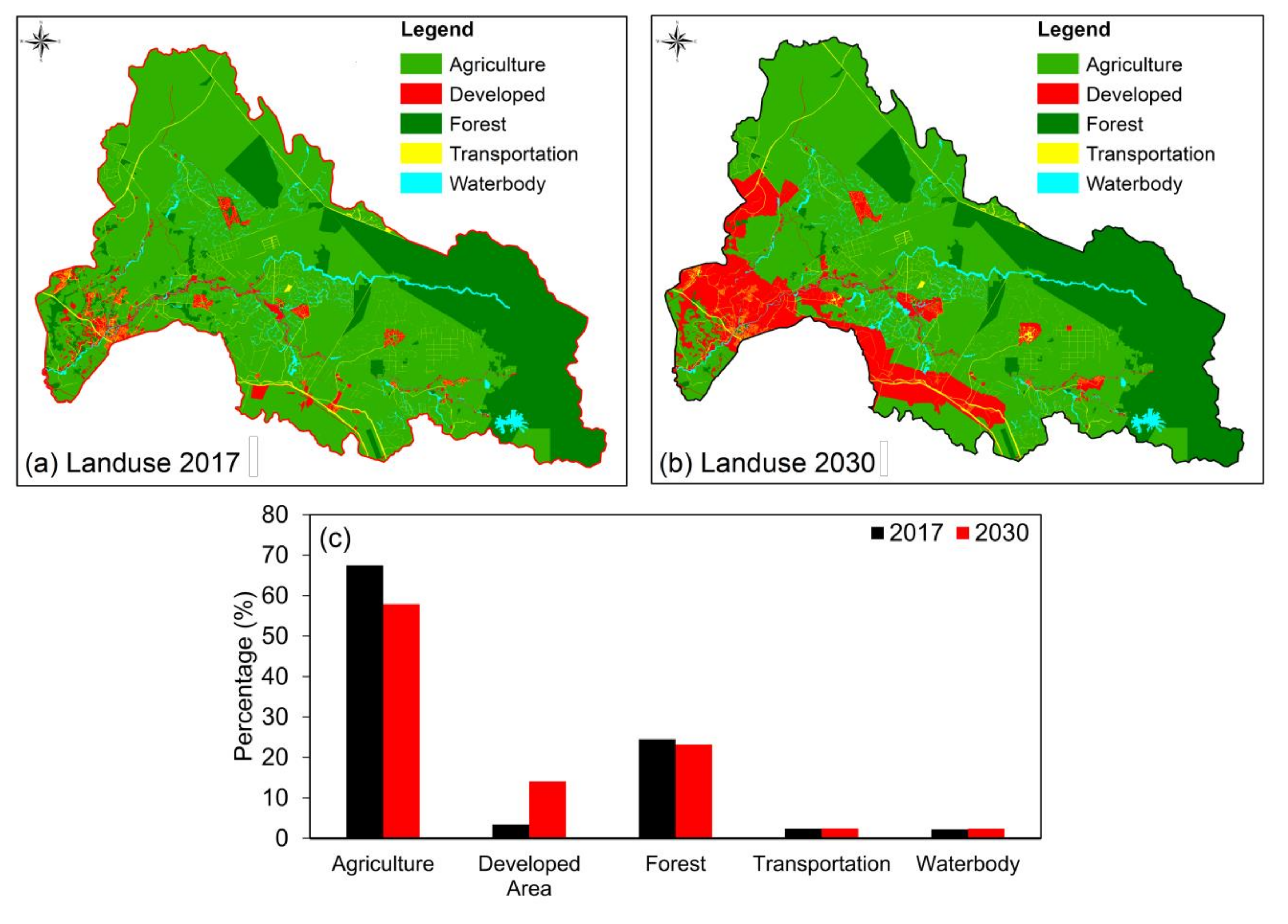
2.3.2. Land Use Change

The projected land use change occurring within the studied basin from 2017 to 2030 was extracted from the draft Johor State Structure Plan 2030 prepared by PlanMalaysia [57] (Figure 3). It is anticipated that major urban development will progress within the river basin. The developed area is expected to increase from 23.69 km² in 2017 (3.38% from the total basin area) to 98.57 km² in 2030 (14.06% from the total basin area). Agricultural land, comprising the majority of the current land use, will decrease dramatically from 473.50 km² in 2017 to 406.06 km² in 2030. Only slight reductions are expected for forests and water bodies due to the policy of maintaining forest reserves and water catchments. The development scenario or the land use change impact scenario (scenario 1) was carried out based on these future land use predictions with simulations using a 12 h critical storm duration. Five land use classes were modeled: agriculture, forests, transportation, water bodies, and settlements, including developed areas. The built-up area covers approximately 60% of the basin’s developed land area.

2.3.3. Climate Change

Climate change is projected to worsen the frequency, intensity, and impacts of some types of extreme weather events that lead to the occurrence of major floods or droughts in an area. Scenario 2 estimates the impacts of climate change on future flooding by referencing the “Estimation of Future Design Rainstorm under the Climate Change Scenario in Peninsular Malaysia” guide, which provides the climate change factor (CCF) variable with which to quantify the scale of climatic changes to surface water systems in 2013, proposed by the National Water Research Institute of Malaysia (NAHRIM) [58]. The CCF is defined as the ratio of the design rainfall for each of the future periods (ratios of time horizons to the control periods of historical rainfall). An approach was introduced in the baseline model to quantify the scale of climatic changes on surface water systems in the future through the development of the CCF and the reformulation of the developed IDF relationship [58]. This approach complied with the use of this guide in the following year for all flood mitigation structural designs established by DID to ensure that they were able to adapt to future climate change scenarios. As a result, the effects of climate change on floods and over the service lives of infrastructure are likely to alter the hydrologic regime and can be considered when determining design flows based upon past historical flow measurements. The magnitude of future design rainfall or rainfall intensity ($I_F$) can be represented by the following empirical equation, as depicted in

Table 3. Climate change factor (CCF) values [58].

No	Station ID	Station Name	10-Year ARI	50-Year ARI	100-Year ARI
1	2330009	Ladang Sungai Labis di Labis	1.39	1.55	1.60
2	2528012	Rumah Tapis Segamat	1.46	1.61	1.66
3	2427001	Felcra Tebing Tinggi di Segamat	1.44	1.60	1.64
4	2527004	Ladang Paya Lang, Segamat	1.43	1.60	1.64
5	2630001	Sungai Pukim	1.35	1.50	1.55

:

$$i=\frac{\lambda T^{\kappa }}{{\left(d+\theta \right)}^{\eta }}$$

(1)

$$I_F=CCF\times \left(i\right)$$

(2)

where i is the average rainfall intensity (mm/hr); T is the average recurrence interval (ARI); d is the storm duration (hours), 0.0833 ≤ d ≤ 72; λ, κ, θ, and η are the fitting constants dependent on the rain gauge location; and $I_F$ is the future design rainfall or rainfall intensity.

2.3.4. Detention Pond Mitigation Scenario

The first mitigation strategy scenario (scenario 3a) was carried out based on six detention ponds (of 3-m depths) with areas ranging from 0.2 km² to 0.8 km². According to Zheng et al. [59], areas with high to moderate runoff are suitable for the use of detention ponds to reduce the flood risk in the lower river basin. Another consideration of site selection is to ensure that the accessibility to readily available forest and agricultural land is made easier and less complicated by regulatory authorities in adopting this proposed mitigation strategy in the future. Therefore, these ponds were proposed in the upper Segamat River Basin, as shown in Figure 4a, to reduce the flood risks in the lower Segamat River Basin, especially in Segamat town.

2.3.5. Rainwater Harvesting System (RWHS) Mitigation Scenario

According to the Johor State Uniform Building (Amendment) By-Laws 2012, it has been mandatory for all new developments in the state to install RWHSs since 2012. As recommended by the Urban Stormwater Management Manual for Malaysia (MSMA) [60], the typical tank size for Malaysia, regardless of location, is 1 m³ for a roof area of 100 m², which is equivalent to storing 10 mm of rainfall with 100 m² of roof area. Hence, the second mitigation strategy scenario (scenario 3b) was carried out with the assumption that 1 m³ rainwater tanks were installed on all residential and commercial buildings in the Segamat River Basin to determine the effects of RWHS application on reducing the flood area. Currently, there are 2786 and 13,763 cadastral lots in the Segamat River Basin classified as commercial and residential lots, respectively (Figure 4b). Commercial lots make up 1.78 km² of the entire basin, and these lots consist of shop lots, supermarkets, shopping complexes, and factories. The residential lots within the basin are terrace houses, village houses, and the base areas of high-rise residential units. The total area of cadastral lots classified as residential made up 8.55 km² of the entire basin. Under the assumed configuration, it is estimated that 16,550 m³ of rainwater can be harvested by RWHSs during major storms.

2.3.6. Permeable Paver Mitigation Scenario

Based on the information provided by the Segamat Municipal Council (MDS), there are a total of 2563 street parking lot units available in the Segamat River basin (Figure 4c).

In general, there are three types of parking lot units in this region: perpendicular, angled echelon, and parallel, with area sizes of 10 × 20 ft. Therefore, the application of permeable pavers for all existing street parking lots in the Sungai Segamat River Basin with a total area of 46,910 m² was done by allowing surface runoff to be captured and infiltrated into the ground, reducing surface runoff accumulation, thus leading to lower flood risks (scenario 3c).

3. Results

3.1. Model Calibration and Validation

There are several flood event records available for this river basin; however, only events with complete recorded rainfall and water level data were used for the model calibration and validation. The calibration process was carried out based on four high-flow events (Figure 5a–d). The peak water level and overall shape of the simulated hydrographs agreed well with the observed data, and thus provided a good basis for storm simulation design. The performance evaluation was carried out in the InfoWorks ICM model by validation with a long-duration simulation at the hourly scale (17 November to 17 December 2010), as shown in Figure 5e.

Table 4. Events considered in the calibration process.

No.	Start Date	End Date	Peak Water Level (m)		Statistical Measures
			Simulated	Observed	RMSE	MAE	R2	NSE
1.	27 January 2004	7 February 2004	8.96	8.66	0.38	0.24	0.96	0.91
2.	27 January 2008	1 February 2008	8.98	9.47	0.30	0.17	0.98	0.97
3.	13 March 2009	18 March 2009	6.39	6.33	0.08	0.06	0.99	0.98
4.	7 April 2009	11 April 2009	6.25	6.25	0.19	0.13	0.95	0.91
5.	17 November 2010	17 December 2010	6.32	6.85	0.15	0.09	0.90	0.88

summarizes the simulated and observed water levels considered in the calibration and validation processes. The statistical measures used were the root mean square error (RMSE), mean absolute error (MAE), coefficient of determination (R²), and Nash–Sutcliffe efficiency (NSE). Overall, the model performance was generally very good for the simulated hourly water level for the 2004 to 2010 storm events at the Segamat River water level station.

After the calibration and validation processes were completed satisfactorily, the flood simulation model was verified by reproducing the 2011 flood, which lasted from 30 January to 4 February 2011, one of the most severe floods that has occurred in recent years. According to Romali et al. [54], the results of the flood frequency analysis show that the 2011 flood was higher than the 50-year flood peaks. Approximately 66% of Segamat town was inundated during the 2011 flood, with water depths of more than 1.2 m causing two fatalities; 28,932 individuals were evacuated from their homes. However, based on the flow data obtained from DID, the peak flow of 5.1 m³/s does not represent the major flood event that occurred in 2011; through historical data, flood peaks recorded during other major floods in 1969, 1979, 1984, and 2007 in the Segamat River Basin were greater than 1000 m³/s. Thus, the simulated peak flow of 1500 m³/s generated from the current flood simulation can be considered an acceptable flow value. Figure 6 illustrates the comparison between the simulated flood depths and the eight observation points in Segamat town collected by Romali et al. [54]. Although IFSAR data were available in this study, the accuracies of the 2D simulations, particularly for the water depths in the inundation area, may not have been accurate. However, the simulated flood water depth results were generally acceptable, with a correlation coefficient value of 0.95, in which a straight line of best fit was superimposed on the scatter plot, as shown in Figure 7. Thus, the model implemented in InfoWorks ICM seems to be a reliable and credible way to reproduce the flood events that have been observed and reported in river basins.

3.2. Scenario Analysis

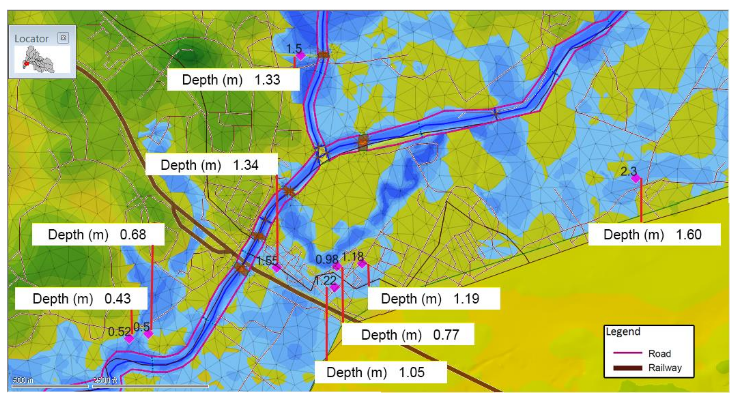
3.2.1. Baseline Model

The analyses for the 10-, 50-, 100-, and 1000-year ARIs with simulations using a 12 h critical storm duration and 2017 land use data were considered as the baseline scenario. The current model simulation, however, did not consider any backwater from the Muar River due to a lack of data for simulating the influences of the Muar River. The results for InfoWorks ICM with respect to the main flood-prone areas were then exported to ArcMap for flood pattern derivations on each floodplain. The total areas for the three flood depths of 0 to 0.5 m, 0.5 to 1.2 m, and more than 1.2 m were extracted and calculated from the flood maps (Figure 8).

Table 5. Potential (maximum) flood-inundated area.

Flood Depth (m)	10-Year ARI		50-Year ARI		100-Year ARI		1000-Year ARI
	Area		Area		Area		Area
	(km2)	(%)	(km2)	(%)	(km2)	(%)	(km2)	(%)
0–0.5	4.02	21.51	4.24	19.99	4.35	19.63	4.45	18.18
0.5–1.2	4.43	23.70	5.08	23.95	5.23	23.60	5.64	23.04
>1.2	10.24	54.79	11.89	56.06	12.58	56.77	14.39	58.78
Total	18.69	100.00	21.21	100.00	22.16	100.00	24.48	100.00

shows the totals and percentages of the inundated areas for various ARIs.

The potential flood-inundated areas were estimated to be 18.69 km², 21.21 km², 22.16 km², and 24.48 km² for 10-, 50-, 100-, and 1000-year ARI storms, respectively. Generally, the flood extent was observed across the floodplain at the downstream stretches of the Segamat River, i.e., chainage 18000 to chainage 0 (Figure 1), corresponding to approximately 75% of the total inundated area of the basin. Comparing the inundation area of the 1000-year ARI storm with those of the 10-, 50-, and 100-ARI storms, the simulation of the 1000-year ARI resulted in the greatest flood-inundated area, classified under extreme hazard conditions. Referring to Table 5, approximately 55% of the flood-inundated areas experienced flood depths above 1.2 m for 10-, 50-, 100-, and 1000-ARI storms. This result shows an increasing trend in terms of flooding area, while ARI storms increased from 10- to 1000-year ARIs.

3.2.2. Land Use Change Impact Scenario

Table 6. Potential (maximum) flood-inundated areas under the land use change scenario.

Flood Depth (m)	10-Year ARI		50-Year ARI		100-Year ARI		1000-Year ARI
	Area		Area		Area		Area
	(km2)	(%)	(km2)	(%)	(km2)	(%)	(km2)	(%)
0–0.5	4.06	20.91	4.26	19.94	4.48	20.07	4.49	18.28
0.5–1.2	4.63	23.83	5.10	23.88	5.20	23.32	5.69	23.13
>1.2	10.74	55.26	12.01	56.18	12.63	56.61	14.40	58.59
Total	19.43	100.00	21.37	100.00	22.31	100.00	24.58	100.00

lists the totals and percentages of the potential inundated areas under various ARIs. Under this scenario, the flood-inundated area was slightly increased compared to the baseline model, as illustrated in Figure 8. The reason behind the increase in the flood-inundated area observed under this scenario was rapid urbanization, particularly in the downstream area, which involved an increase in the CN value. The potential flood-inundated areas were estimated to be 19.43 km², 21.37 km², 22.31 km², and 24.58 km² for storms of 10-, 50-, 100-, and 1000-year ARIs, respectively.

3.2.3. Climate Change Impact Scenario

Table 7. Potential (maximum) flood-inundated area under the climate change impact scenario.

Flood Depth (m)	10-Year ARI + CCF		50-Year ARI + CCF		100-Year ARI + CCF
	Area		Area		Area
	(km2)	(%)	(km2)	(%)	(km2)	(%)
0–0.5	4.27	20.35	4.48	18.11	4.59	18.35
0.5–1.2	5.09	24.26	5.77	23.32	5.68	22.71
>1.2	11.62	55.39	14.49	58.57	14.74	58.94
Total	20.98	100.00	24.74	100.00	25.01	100.00

depicts the totals and percentages of the potential (maximum) inundated areas for various ARIs under climate change and the present land use conditions. Regarding this aspect, the modeled peak discharges significantly increased for all sub-basins, and the potential flood-inundated area is likely to be larger under the climate change scenario than the flood-inundated-area under the baseline model or land use change impact scenarios; with climate change trends, the values are estimated to be 20.98 km², 24.74 km², and 25.01 km² for storms of 10-, 50-, and 100-year ARIs, respectively. In particular, when CCF was performed for a 50-year ARI storm, the potential flood-inundated area was estimated at 24.74 km², which was already more severe than all potential flood-inundated areas for storms of 50-, 100-, and 1000-year ARIs under the baseline scenario and land use change impact scenario. This scenario clearly demonstrates that the IDF curves of the designed storms were updated when implementing CCF, resulting in higher rainfall depths and intensities; subsequently, the simulation of the 1000-year ARI was not performed with CCF in the current study.

3.2.4. Mitigation Strategy Scenarios

The resulting totals and percentages of the potential (maximum) inundated areas for various ARIs under the three mitigation strategies, namely the provision of detention ponds, the installation of RWHSs, and the installation of permeable pavers, are shown in

Table 8. Potential (maximum) flood-inundated areas under different mitigation strategy scenarios.

Flood Depth (m)	10-Year ARI		50-Year ARI		100-Year ARI		1000-Year ARI
	Area		Area		Area		Area
	(km2)	(%)	(km2)	(%)	(km2)	(%)	(km2)	(%)
(a) Scenaroi 3a—Detention Ponds
0–0.5	3.16	20.37	4.04	21.12	4.07	20.44	4.15	19.45
0.5–1.2	3.70	23.86	4.62	24.15	4.79	24.06	5.02	23.52
>1.2	8.65	55.77	10.47	54.73	11.05	55.50	12.17	57.03
Total	15.51	100.00	19.13	100.00	19.91	100.00	21.34	100.00
(b) Scenaroi 3b—Rainwater Harvesting System (RWHS)
0–0.5	4.03	20.67	4.32	20.09	4.35	19.73	4.47	18.33
0.5–1.2	4.65	23.84	5.12	23.82	5.17	23.44	5.65	23.16
>1.2	10.82	55.49	12.06	56.09	12.53	56.83	14.27	58.51
Total	19.50	100.00	21.50	100.00	22.05	100.00	24.39	100.00
(c) Scenaroi 3c—Permeable Pavers
0–0.5	4.05	21.24	4.23	20.15	4.36	19.53	4.45	18.02
0.5–1.2	4.53	23.75	5.00	23.82	5.29	23.69	5.71	23.13
>1.2	10.49	55.01	11.76	56.03	12.68	56.78	14.53	58.85
Total	19.07	100.00	20.99	100.00	22.33	100.00	24.69	100.00
(d) Scenaroi 4a—Detention Ponds, RWHS, and Permeable Pavers
0–0.5	3.37	21.04	4.02	20.98	4.06	20.47	4.15	19.17
0.5–1.2	3.82	23.85	4.63	24.17	4.76	24.02	5.11	23.63
>1.2	8.83	55.12	10.52	54.86	11.00	55.51	12.38	57.20
Total	16.02	100.00	19.17	100.00	19.82	100.00	21.64	100.00
(e) Scenaroi 4b—Detention Ponds, RWHS, and Permeable Pavers under Climate Change Impact Scenario
0–0.5	4.03	20.84	4.21	19.05	4.17	18.43	-	-
0.5–1.2	4.66	24.11	5.19	23.49	5.34	23.61	-	-
>1.2	10.65	55.04	12.69	57.46	13.12	57.96	-	-
Total	19.34	100.00	22.09	100.00	22.63	100.00

. The aforementioned results revealed that there were significant reduction in the flood-inundated areas under the detention pond mitigation strategy. Under this condition, the potential flood-inundated areas were estimated to be 15.51 km², 19.13 km², 19.91 km², and 21.34 km² for storms of 10-, 50-, 100-, and 1000-year ARIs, respectively. In contrast, there were no significant differences observed in the inundation areas between the RWHS or permeable paver scenario and the baseline scenario. For instance, the proposed RWHSs and permeable pavers resulted in inundated areas of 24.39 km² and 24.69 km² for the 1000-year ARI storm, respectively. Approximately 14.2 km² to 14.5 km² of land had water depths of more than 1.2 m. Indeed, the inundated area predicted under the highest flood depth scenario was also the largest size for all three scenarios (>55%). Similarly, the estimated flood-inundated area was very close to that reported in scenario 3a when the three mitigation types, namely detention ponds, RWHSs, and permeable pavers, were combined. The potential flood-inundated areas were estimated to be 16.02 km² to 21.64 km² for storms of 10- to 1000-year ARIs under scenario 4a and 19.34 km² to 22.63 km² for storms of 10- to 100-year ARIs under scenario 4b.

Respective flood maps were produced separately from the current study based on the three scenarios after the completion of the baseline simulation; these flood maps highlighted the extent and depth of inundation.

Table 9. Potential (maximum) flood-inundated area.

Design Storm	Scenario	Flood-Inundated Area (km2)	Relative Change (%)
10-Year ARI	Baseline	18.69
	Scenario 1	19.43	3.96
	Scenario 2	20.98	12.25
	Scenario 3a	15.51	−17.01
	Scenario 3b	19.50	4.33
	Scenario 3c	19.07	2.03
	Scenario 4a	16.02	−14.29
	Scenario 4b	19.34	−7.82
50-Year ARI	Baseline	21.21
	Scenario 1	21.37	0.75
	Scenario 2	24.74	16.64
	Scenario 3a	19.13	−9.81
	Scenario 3b	21.50	1.37
	Scenario 3c	20.99	−1.04
	Scenario 4a	19.17	−9.62
	Scenario 4b	22.09	−10.71
100-Year ARI	Baseline	22.16
	Scenario 1	22.31	0.68
	Scenario 2	25.01	12.86
	Scenario 3a	19.91	−10.15
	Scenario 3b	22.05	−0.50
	Scenario 3c	22.33	0.77
	Scenario 4a	19.82	−10.56
	Scenario 4b	22.63	−9.52
1000-Year ARI	Baseline	24.48
	Scenario 1	24.58	0.41
	Scenario 2	-	-
	Scenario 3a	21.34	−12.83
	Scenario 3b	24.39	−0.37
	Scenario 3c	24.69	0.86
	Scenario 4a	21.64	−11.60
	Scenario 4b	-	-

summarizes the total potential inundated areas predicted under various scenarios and ARIs. The results revealed that the flood risk will increase significantly under both urbanization (scenario 1) and climate change (scenario 2). The urban area is expected to increase significantly in the downstream region by 2030, reaching a total area of 98.57 km². The results show that overall impact of urbanization on the flood extent is rather moderate compared to that shown in the baseline model due to the reduction of flood flow by the large forestland and agricultural areas in the upstream region. Under the climate change impact scenario, the potential flood-inundated area is expected to increase from 12.25% to 16.64% under simulations of storms with 10-, 50-, and 100-year ARIs.

4. Discussion

The results for the simulated peak discharges of the sub-basins (refer to Appendix B) motivated us to carry out the hydrological model to assess how each sub-basin contributes to the peak discharge under different return periods and scenarios. Investigations of the responses of the Segamat River Basin to different scenarios are discussed in these sections. An analysis of the changes in the peak flows of the model outputs was carried out by checking the flow ratio between the baseline model and the simulations. Climate change impacts (scenario 2) were found to contribute the most to producing peak flows for all sub-basins, while increased urbanization (scenario 1) came in second place. The land use and climate change impact scenarios increased the peak runoff values from 11.5% to 23.2% and from 27.7% to 44.2%, respectively, under all investigated storm ARIs. In short, the present study has shown that climate change is dominant over all other factors and has a significant impact on hydrological changes in the Segamat River Basin, mainly caused by the CCF variables and increased precipitation. Thus, the analyses of the aggregated impacts of climate change (scenario 2) resulted in higher peak flows and greater flood extents compared to the land use change scenario (scenario 1). Moreover, the Segamat River Basin is a typical rural basin in Johor State, and agricultural activities dominate in the basin. The impact of future land use changes with respect to the conversion of agricultural land into development land accounted for approximately 10% in the lower river basin, while the area of agricultural land decreased from 473.50 km² to 406.06 km² when we compared the land use situation in 2017 to that in 2030. Although urbanization has increased significantly based on future land use in 2030, the overall impact of urbanization on the flood extent is rather moderate (increase of 0.1 km²), because the upstream part of the basin is dominated largely by forested lands and areas used for agricultural activities (81.13%).

Noticeably, the peak flow ratios with respect to the effects of the provision of detention ponds (scenario 3a) by storing runoff in the detention ponds will reduce the peak runoff rate by approximately 1% under storms of 10-, 50-, 100-, and 1000-year ARIs. Generally, scenario 3a demonstrated the ability of flood storage to reduce peak discharges by a small but obvious amount for high-flow events. Detention ponds are a popular stormwater management practice in many communities [61], being designed to store and release the runoff of extreme rainfall events. Their main function is to regulate the runoff from flowing further downstream and offer flood protection to the downstream communities. The simulation results for the six proposed detention ponds in the river basin showed that approximately 6% to 17% of the flooded area can be reduced with the implementation of detention ponds. In addition, the flood ponds were effective at reducing peak discharges immediately downstream of their headwater locations and slowing down the time to peak discharge. In addition, detention ponds in such agricultural-dominated river basins also provide a sustainable and cost-effective alternative to irrigation purposes, as they extend the potential water reuse schemes to farmers.

Interestingly, the results for the construction of rainwater harvesting systems (RWHS) and permeable pavers under scenarios 3b and 3c demonstrated that the contributions of RWHSs and permeable pavers to flood volume reductions are not encouraging due to the limitations of the capacity of these methods to store rainfall during peak events. Specifically, RWHSs and permeable pavers have remarkable roles in the reduction of flood volumes for storms of smaller ARIs and provide important contributions to stormwater management, such as avoiding potential drainage system failures during storm events. Nevertheless, the effectiveness of these systems is affected by the magnitude of storm events. Under major storm events, the RWHSs and permeable pavers are unable to offer good performance due to large volumes of surface runoff being generated over the entire river basin. Indeed, the capacity of RWHSs and permeable pavers in scenarios 3b and 3c to harvest or capture the runoff volumes for storms of 10- to 1000-year ARIs is generally relatively low compared with the total storage volume of the detention ponds (14.85 million m³) explored in scenario 3a.

Likewise, the combination of the three mitigation strategies of detention ponds, RWHSs, and permeable pavers results in a substantial reduction in the extent of the flood area compared with the baseline scenario; this reduction is similar to that reported in scenario 3a. The total reductions in the flood inundation area for the combination of three means of mitigation measures under scenario 4a are 14.29%, 9.62%, 10.56%, and 11.60% for storms of 10-, 50-, 100-, and 1000-year ARIs, respectively. On the other hand, the total reductions in the flood-inundated area for the combination of the three mitigation strategies under scenario 4b are 7.82%, 10.71, and 9.52% for storms of 10-, 50-, and 100-year ARIs (compared with those of scenario 2 under the climate change impact scenario). Generally, there is no significant difference between the combination of the three mitigation strategies and the detention pond strategy alone on flood inundation reduction. As a result, compared to RWHSs and permeable pavers, detention ponds are the only dominant flood mitigation strategy and should be prioritized for flood hazard mitigation, as reported in scenarios 3a, 4a, and 4b.

5. Conclusions

Flood maps are the basic tools and starting points used to design flood management policies; they will be instrumental for government and local authorities, such as urban planning departments, in ascertaining potential flood damages to properties and the extent of the disruption to economic activities more accurately, as well as in facilitating the implementation of flood mitigation measures, controls, and management to achieve security, quality, and sustainability in river basins. Another focus of this study was to assess the validity of four scenarios in order to develop a more advanced hydrodynamic model. The current study successfully formulated digital flood maps for storms of 10-, 50-, 100-, and 1000-year ARIs using 2017 land use data for the Segamat River Basin. InfoWorks ICM was calibrated and validated for several historical, high-flow, and flood events that occurred in the Segamat River Basin to assess the extent of flood risk in the basin, with significant 12 h critical storm events (10-, 50-, 100-, and 1000-year ARIs) based on four scenarios.

The impacts of land use change and climate change on the peak flows for each sub-basin and the reductions in flood inundation predicted under various scenarios were determined using the results from the baseline model to provide benchmarks in the river basin. The current study was revealed and confirmed by a literature search, which indicated that land use and climate change tend to have greater impacts on peak flood flows than other factors, further corroborating urbanization- and climate change-induced intensifying flood processes in studies on flood probability and flood consequences. The highest flood risk was observed in the downstream region of the Segamat River Basin. The flood inundation extent and depths predicted under future land use conditions and with climate change impacts were significantly higher (up to 18%) than those of the baseline model. These findings clearly emphasize the need for further flood protection and mitigation measures towards sustainable development. With the proposed quantity control and mitigation strategies, the current study attempted to establish an understanding of the inundated areas and flood depths in the Segamat River Basin. The six proposed detention ponds in the river basin provided promising results in terms of reducing peak discharges and flood volumes; an estimated 6% to 17% of the flooded area was reduced. Consequently, the proposed mitigation strategy was in line with MSMA runoff quantity control requirements, in which detention storage facilities are the core elements required to achieve major stormwater quantity control, and therefore are promoted by local regulatory authorities in urban planning to ensure that all development projects shall be protected against both minor and major floods [60]. In contrast, the installation of RWHSs and permeable pavers demonstrated lesser impacts in reducing flood risks. The present study clearly outlined the limitations of the application of these systems in urban areas specifically located in the lower river basin (residential and commercial areas), as the basin scale is relatively small in terms of harvesting volume, while the proposed mitigation measures are also affected by the magnitudes of rainfall events. Therefore, it is suggested that further studies should be conducted to more deeply explore the advantages of having RWHSs and permeable pavers, as well as other best management practices, such as swales, bioretention strategies, and constructed wetlands, in order to determine the benefits these strategies will provide as flood reduction measures through a distributed rainfall–runoff model. In addition, future research should also focus on interdisciplinary flood risk research on flood probability and the extent of economic damage and vulnerability.

References

1. IPCC. Managing the Risks of Extreme Events and Disasters to Advance Climate Change Adaptation. A Special Report of Working Groups I and II of the Intergovernmental Panel on Climate Change; Field, C.B., Barros, V., Stocker, T.F., Qin, D., Dokken, D.J., Ebi, K.L., Mastrandrea, M.D., Mach, K.J., Plattner, G.-K., Allen, S.K., et al., Eds.; Cambridge University Press: Cambridge, UK; New York, NY, USA, 2012; p. 582. [Google Scholar]
2. Li, X.; Wang, X.; Babovic, V. Analysis of variability and trends of precipitation extremes in Singapore during 1980–2013. Int. J. Climatol. 2017, 38, 125–141. [Google Scholar] [CrossRef]
3. Mayowa, O.O.; Pour, S.H.; Shahid, S.; Mohsenipour, M.; Harun, S.B.; Heryansyah, A.; Ismail, T. Trends in rainfall and rainfall-related extremes in the east coast of peninsular Malaysia. J. Earth Syst. Sci. 2015, 124, 1609–1622. [Google Scholar] [CrossRef] [Green Version]
4. Santosh, F.B.; Ramesh, H. Analysis of South West monsoon rainfall trend using statistical techniques over Nethravathi Basin. Int. J. Adv. Technol. Civil Eng. 2013, 2, 130–136. [Google Scholar]
5. Tan, M.L.; Ibrahim, A.L.; Cracknell, A.P.; Yusop, Z. Changes in precipitation extremes over the Kelantan River Basin, Malaysia. Int. J. Climatol. 2017, 37, 3780–3797. [Google Scholar] [CrossRef]
6. Karmeshu, N. Trend Detection in Annual Temperature and Precipitation using the Mann Kendall Test—A Case Study to Assess Climate Change on Select States in the Northeastern United States. Master’s Thesis, University of Pennsylvania, Philadelphia, PA, USA, 2012. [Google Scholar]
7. Liew, Y.S.; Teo, F.Y. Impact of Climate Change on Flooding Scenario in Segamat River Basin, Malaysia. In Proceedings of the World Engineers Summit (WES2013): Innovative and Sustainable Solutions to Climate Change, Singapore, 9–15 September 2013; pp. 153–158. [Google Scholar]
8. Al-Houri, Z. Detecting variability and trends in daily rainfall characteristics in Amman-Zarqa basin, Jordan. Int. J. Appl. Sci. Technol. 2014, 4, 11–23. [Google Scholar]
9. Kiros, G.; Shetty, A.; Nandagiri, L. Extreme Rainfall Signatures under. Changing Climate in Semi-arid Northern Highlands of Ethiopia. Cogent Geosci. 2017, 1353719. [Google Scholar] [CrossRef]
10. Tan, M.L.; Yusop, Z.; Chua, V.P.; Chan, N.W. Climate change impacts under CMIP5 RCP scenarios on water resources of the Kelantan River Basin, Malaysia. Atmos. Res. 2017, 189, 1–10. [Google Scholar] [CrossRef]
11. Chan, N.; Tan, M.; Ghani, A.; Zakaria, N. Sustainable Urban Drainage as a Viable Measure of Coping with Heat and Floods Due to Climate Change. In IOP Conference Series: Earth and Environmental Science; IOP Publishing: Bristol, UK, 2019. [Google Scholar] [CrossRef]
12. Samuels, P.G. Risk and Uncertainty in Flood Management. In River Basin Modelling for Flood Risk Mitigation; Knight, D.W., Shamseldin, A.Y., Eds.; Taylor & Francis Group plc.: London, UK, 2006. [Google Scholar]
13. White, G.F.; Haas, J.E. Assessment of Research on Natural Hazards; MIT Press: Cambridge, MA, USA, 1975. [Google Scholar]
14. Freni, G.; Liuzzo, L. Effectiveness of Rainwater Harvesting Systems for Flood Reduction in Residential Urban Areas. Water 2019, 11, 1389. [Google Scholar] [CrossRef] [Green Version]
15. Cristiano, E.; Farris, S.; Deidda, R.; Viola, F. Comparison of blue-green solutions for urban flood mitigation: A multi-city large-scale analysis. PLoS ONE 2021, 16, e0246429. [Google Scholar] [CrossRef] [PubMed]
16. Burns, M.J.; Fletcher, T.D.; Duncan, H.P.; Hatt, B.E.; Ladson, A.R.; Walsh, C.J. The stormwater retention performance of rainwater tanks at the landparcel scale. In Proceedings of the 7th International Conference on Water Sensitive Urban Design, Melbourne, Australia, 21–23 February 2012; p. 195. [Google Scholar]
17. Coombes, P.J. and Barry, M.E. The relative efficiency of water supply catchments and rainwater tanks in cities subject to variable climate and the potential for climate change. Australas. J. Water Resour. 2008, 12, 85–100. [Google Scholar] [CrossRef]
18. Steffen, J.; Jensen, M.; Pomeroy, C.A.; Burian, S.J. Water Supply and Stormwater Management Benefits of Residential Rainwater Harvesting in U.S. Cities. J. Am. Water Resour. Assoc. (Jawra) 2013, 49, 810–824. [Google Scholar] [CrossRef]
19. Md Lani, N.H.; Yusop, Z.; Syafiuddin, A. A review of rainwater harvesting in Malaysia: Prospects and challenges. Water 2018, 10, 506. [Google Scholar] [CrossRef] [Green Version]
20. Ferguson, B. Porous Pavements; CRC Press: Boca Raton, FL, USA, 2005. [Google Scholar]
21. Zabidi, H.A.; Goh, H.W.; Chang, C.K.; Chan, N.W.; Zakaria, N.A. A Review of Roof and Pond Rainwater Harvesting System: The Design, Performance and Way Forward. Water 2020, 12, 3163. [Google Scholar] [CrossRef]
22. Thomas, D.; Benjamin, G. Flood risk management in Europe and the development of a common EU policy. Int. J. River Basin Manag. 2005, 3, 97–103. [Google Scholar] [CrossRef]
23. Merz, B.; Hall, J.; Disse, M.; Schumann, A. Fluvial flood risk management in a changing world. Nat. Hazards Earth Syst. Sci. 2010, 10, 509–527. [Google Scholar] [CrossRef] [Green Version]
24. Heintz, M.D.; Hagemeier-Klose, M.; Wagner, K. Towards a Risk Governance Culture in Flood Policy—Findings from the Implementation of the “Floods Directive” in Germany. Water 2012, 4, 135–156. [Google Scholar] [CrossRef] [Green Version]
25. Caddis, B.; Nielsen, C.; Wedge, H.; Tahir, P.A.; Teo, F.Y. Guidelines for floodplain development—A Malaysian case study. Int. J. River Basin Manag. 2012, 10, 161–170. [Google Scholar] [CrossRef]
26. Dinh, Q.; Balica, S.; Popescu, I.; Jonoski, A. Climate change impact on flood hazard, vulnerability and risk of the Long Xuyen Quadrangle in the Mekong Delta. Int. J. River Basin Manag. 2012, 10, 103–120. [Google Scholar] [CrossRef]
27. Cvetkovic, V.; Martinovic, J. Innovative Solutions for Flood Risk Management. Int. J. Disaster Risk Manag. 2021, 2. [Google Scholar] [CrossRef]
28. Adnan, M.S.G.; Md Abdullah, A.Y.; Dewan, A.; Hall, J.W. The effects of changing land use and flood hazard on poverty in coastal Bangladesh. Land Use Policy 2020, 99, 104868. [Google Scholar] [CrossRef]
29. Department of Irrigation and Drainage Malaysia (DID). Segamat 2006/2007 Flood Report; Department of Irrigation and Drainage of Johor: Johor Bharu, Malaysia, 2007. [Google Scholar]
30. Gasim, M.B.; Surif, S.; Mokhtar, M.; Toriman, M.E.; Abd Rahim, S.S.; Bee, C.H. Analisis Banjir Disember 2006: Tumpuan di Kawasan Bandar Segamat, Johor. Sains. Malays. 2010, 39, 353–361. [Google Scholar]
31. Aboelnour, M.; Gitau, M.W.; Engel, B.A. A Comparison of Streamflow and Baseflow Responses to Land-Use Change and the Variation in Climate Parameters Using SWAT. Water 2020, 12, 191. [Google Scholar] [CrossRef] [Green Version]
32. Talib, A.; Randhir, T.O. Climate change and land use impacts on hydrologic processes of watershed systems. J. Water Clim. Chang. 2017, 8, 363–374. [Google Scholar] [CrossRef]
33. Khoi, D.N.; Nguyen, V.T.; Sam, T.T.; Nhi, P.T.T. Evaluation on Effects of Climate and Land-Use Changes on Streamflow and Water Quality in the La Buong River Basin, Southern Vietnam. Sustainability 2019, 11, 7221. [Google Scholar] [CrossRef] [Green Version]
34. Liu, J.; Xue, B.; Yan, Y. The Assessment of Climate Change and Land-Use Influences on the Runoff of a Typical Coastal Basin in Northern China. Sustainability 2020, 12, 10050. [Google Scholar] [CrossRef]
35. Romali, N.S.; Yusop, Z. Flood damage and risk assessment for urban area in Malaysia. Hydrol. Res. 2020, nh2020121. [Google Scholar] [CrossRef]
36. Ahmed, K.; Chung, E.S.; Song, J.Y.; Shahid, S. Effective Design and Planning Specification on Low Impact Development Practices using Water Management Analysis Module (WMAM): Case of Malaysia. Water 2017, 9, 173. [Google Scholar] [CrossRef] [Green Version]
37. Rezaei, A.R.; Ismail, Z.; Niksokhan, M.H.; Dayarian, M.A.; Ramli, A.H.; Shirazi, S.M. A Quantity-Quality Model to assess the effects of source control stormwater management on hydrology and water quality at the catchment scale. Water 2019, 11, 1415. [Google Scholar] [CrossRef] [Green Version]
38. Finaud-Guyol, P.; Delenne, C.; Guinot, V.; Llovel, C.; Mecanique, C.R. 1D–2D coupling for river flow modeling. Comptes Rendus Mécanique 2005, 339, 226–234. [Google Scholar] [CrossRef] [Green Version]
39. Liu, Q.; Qin, Y.; Zhang, Y.; Li, Z. A coupled 1D-2D hydrodynamic model for flood simulation in flood detention basin. Nat. Hazards 2015, 75, 1303–1325. [Google Scholar] [CrossRef]
40. Dasallas, L.; Kim, Y.; An, H. Case Study of HEC-RAS 1D–2D Coupling Simulation: 2002 Baeksan Flood Event in Korea. Water 2019, 11, 2048. [Google Scholar] [CrossRef] [Green Version]
41. Verwey, A. Latest development in floodplain modelling—1D/2D integration. In Proceedings of the Australia Conference on Hydraulics in Civil Engineering, The Institute of Engineers, Hobart, Tasmania, 28–30 November 2001. [Google Scholar]
42. Leow, C.S.; Abdullah, R.; Zakaria, N.A.; Ghani, A.; Chang, C.K. Modelling Urban River Catchment: A Case Study in Malaysia. Water Manag. J. 2009, 162, 25–34. [Google Scholar] [CrossRef]
43. Ziarh, G.F.; Asaduzzaman, M.; Dewan, A.; Nashwan, M.S.; Shahid, S. Integration of Catastophe and entropy theories for flood risk mapping in Peninsular Malaysia. J. Flood Risk Manag. 2021, 14, e12686. [Google Scholar] [CrossRef]
44. Department of Irrigation and Drainage Malaysia (DID). The Preparatory Survey for Integrated River Basin Management Incorporating Integrated Flood Management with Adaptation of Climate Change. Final Report; Volume 2—Muar River Basin; Department of Irrigation and Drainage Malaysia (DID): Kuala Lumpur, Malaysia, 2011. [Google Scholar]
45. Department of Irrigation and Drainage or DID Malaysia. Hydrological Procedure No. 1: Estimation of Design Rainstorm in Peninsular Malaysia; Department of Irrigation and Drainage Malaysia (DID): Kuala Lumpur, Malaysia, 2015. [Google Scholar]
46. United States Department of Agriculture or USDA. Urban Hydrology for Small Watersheds. Technical Release No. 55; USDA, Soil Conservation Service: Washington, DC, USA, 1986. [Google Scholar]
47. Chow, V.T.; Maidment, D.R.; Mays, L.W. A Text Book of Applied Hydrology; Tata McGraw Hill Publications: New Delhi, India, 1988. [Google Scholar]
48. Mishra, S.K.; Singh, V. Soil Conservation Service Curve Number (SCS-CN) Methodology, 42; Springer Science & Business Media: Berlin/Heidelberg, Germany, 2013. [Google Scholar]
49. Chin, S.L. Estimation of Runoff using NRCS Curve Number Method in Oil Palm Catchment. Master’s Thesis, Universiti Teknologi Malaysia, Johor, Malaysia, 2006. [Google Scholar]
50. De Winnaar, G.; Jewitt, G.P.W.; Horan, M. A GIS-based approach for identifying potential runoff harvesting sites in the Thukela River basin, South Africa. Phys. Chem. Earth. 2007, 32, 1058–1067. [Google Scholar] [CrossRef]
51. Luxon, N.; Pius, C. Validation of the rainfall-runoff SCS-CN model in a catchment with limited measured data in Zimbabwe. Int. J. Water Resour. Environ. Eng. 2013, 5, 295–303. [Google Scholar] [CrossRef]
52. National Water Research Institute of Malaysia (NAHRIM). Research of Climate Change Impact on Water Quantity Aspect Towards Achieving Security, Quantity and Sustainability of River System And Balance in River Morphology for Segamat River, Muar River Basin. Final Report; National Water Research Institute of Malaysia (NAHRIM): Seri Kembangan, Selangor, Malaysia, 2020. [Google Scholar]
53. Innovyze. Infoworks ICM. Available online: https://www.innovyze.com/en-us/products/infoworks-icm (accessed on 10 June 2020).
54. Romali, N.S.; Yusop, Z.; Ismail, A.Z. Application of HEC-RAS and Arc GIS for floodplain mapping in Segamat town, Malaysia. Int. J. 2018, 15, 7–13. [Google Scholar] [CrossRef]
55. Department of Irrigation and Drainage Malaysia (DID). Study on River Sand Mining Capacity in Malaysia. Main Report; Department of Irrigation and Drainage Malaysia (DID): Kuala Lumpur, Malaysia, 2009. [Google Scholar]
56. French, R.H. Open Channel Hydraulics; McGraw-Hill Education: New York, NY, USA, 1986. [Google Scholar]
57. Department of Town and Country Planning, PLANMalaysia@Johor. Draft Johor State Structure Plan 2030 (DRSNJ2030). Available online: https://jpbd.johor.gov.my/index.php/intranet/9-uncategorised/122-state-structure-plan (accessed on 29 August 2020).
58. National Hydraulic Research Institute of Malaysia (NAHRIM). Estimation of Future Design Rainstorm under the Climate Change Scenario in Peninsular Malaysia. NAHRIM Technical Guide No.1; National Water Research Institute of Malaysia (NAHRIM): Seri Kembangan, Selangor, Malaysia, 2013. [Google Scholar]
59. Zheng, H.; Gao, J.; Xie, G.; Jin, Y.; Zhang, B. Identifying important ecological areas for potential rainwater harvesting in the semi-arid area of Chifeng, China. PLoS ONE 2018, 13. [Google Scholar] [CrossRef] [PubMed]
60. Department of Irrigation and Drainage or DID Malaysia. Urban Stormwater Management for Malaysia (MSMA), 2nd ed.; Department of Irrigation and Drainage Malaysia (DID): Kuala Lumpur, Malaysia, 2012. [Google Scholar]
61. Goff, K.; Gentry, R. The influence of watershed and development characteristics on the cumulative impacts of stormwater detention ponds. Water Resour. Manag. 2006, 20, 829–860. [Google Scholar] [CrossRef]
62. Miller, J.E. Basic Concepts of Kinematic-Wave Models (No. 1302); US Geological Survey: Washington, DC, USA, 1984. [Google Scholar]
Figure 1. Segamat River Basin.
Sustainability 13 03286 g001
Figure 2. Relevant basin information for the assignment of curve number values: (a) delineated sub-basins of the Segamat River; (b) hydrology soil group map [52].
Sustainability 13 03286 g002
Figure 3. Distributions of the locations of the projected future land use changes within the Segamat River Basin: (a) land use map for 2017; (b) land use map for 2030; (c) projected land use changes from 2017 to 2030 [52].
Sustainability 13 03286 g003
Figure 4. Locations of the (a) detention ponds, (b) rainwater harvesting systems, and (c) permeable pavers in the Segamat River Basin.
Sustainability 13 03286 g004
Figure 5. Comparison between simulated and observed water levels: (a) 27 January to 7 February 2004; (b) 27 January to 1 February 2008; (c) 13 to 18 March 2009; (d) 7 to 11 April 2009; (e) 17 November to 17 December 2010.
Sustainability 13 03286 g005
Figure 6. Validation of flood locations between simulated and observed data [52]. The pink diamond shapes and values represent observation points and water depth (in meters); the values in text boxes represent the simulated water depths (in meters).
Sustainability 13 03286 g006
Figure 7. Comparison of flood water depths between the simulation results and observations of the 2011 flood event.
Sustainability 13 03286 g007
Figure 8. Flood maps of the Segamat River Basin with 2017 land use (ARI): 10-year ARI; (b) 50-year ARI; (c) 100-year ARI; (d) 1000-year ARI [52].
Sustainability 13 03286 g008