A Global Dynamic Harmony Search for Optimization of a Hybrid Photovoltaic-Battery Scheme: Impact of Type of Solar Panels

Abstract

The type of solar panels has a great impact on the optimal sizing of a hybrid photovoltaic–battery scheme. The optimization of these schemes based on a powerful optimization approach results in more cost-effective schemes. In this paper, a new global dynamic harmony search method, as an optimization method, is presented for the optimal sizing of a hybrid photovoltaic–battery scheme. The new optimization method is aimed at minimizing the total cost and loss of load supply probability of the scheme at the same time. In this regard, the effect of the type of solar panels on the optimal sizing of the hybrid scheme is investigated. Furthermore, performance optimizations are performed with an original global dynamic harmony search, an original harmony search, and simulated annealing to determine the effectiveness of the suggested optimization method. The effects of the initial costs and efficiency of monocrystalline and polycrystalline solar panels on the optimization of hybrid systems are analyzed. The superiority of the suggested method in terms of time and cost indicators of the hybrid scheme is presented comparing the other algorithm.

1. Introduction

Renewable energies, as one of the alternative energy sources of fossil fuels, have attracted many researchers as a source of endless energy in the world [1,2]. Among the renewable energies, solar energy has received wide attention and research in the world in recent years. The vigorous development of solar power generation can slow down the consumption of fossil fuels and is of great significance to reduce environmental pollution. Solar energy sources, especially PV panel systems, are applicable for off-grid and on-grid power generation. PV panel systems are suitable for supplying the load demand in stand-alone and remote areas as a clean and cost-effective system [3].

However, due to the uncontrollability and randomness of solar energy, solar power generation makes it difficult to meet the load demand in remote areas, which brings great challenges to the reliable and safe operation of solar power generation systems. To solve this problem, it is necessary to use energy storage and backup units. In this regard, battery energy storage is usually used for electricity storage in remote areas as a backup system [4,5,6,7,8,9,10,11]. Therefore, the hybrid photovoltaic–battery scheme is suggested for the reliable and safe operation of solar power generation systems in remote areas [12,13,14,15].

In order to improve the utilization efficiency of solar energy and realize the cost-effective, safe, and reliable operation of hybrid photovoltaic–battery systems, it is necessary to provide accurate modeling and powerful optimization algorithm. At the same time, using a suitable solar panel is beneficial to hybrid photovoltaic–battery systems. The photovoltaic panel systems can fit into three categories: monocrystalline (Mono-SI), polycrystalline (Poly-SI), and thin-film PV panels. Mono-SI panels have the highest efficiency (16.5–24%) in direct sunlight and are the most expensive and spatially efficient. Polycrystalline panels have lower prices and efficiency (about 12–16%) compared to Mono-SI panels and lower spatial efficiency. Thin-film solar panels are the cheapest and least efficient (about 6–8%) compared to the others [16]. Thus, Mono-SI and Poly-SI solar panels are suggested for the reliable and safe operation of the hybrid photovoltaic–battery system in remote areas.

In recent years, experts have done much research on the investigation of hybrid schemes with solar energy. Symeonidou et al. [17] presented a mathematical tool to manage the energy produced by the residential on-grid hybrid photovoltaic–battery system. It is found that storage is a feasible selection whenever selling power to the main grid is not appropriate. Karamov and Suslov [18] presented a methodology based on the Chronological modeling method for optimization of the stand-alone hybrid photovoltaic–battery scheme. It is found that the combined use of photovoltaics and batteries reduces diesel fuel consumption by 51%. Bhayo et al. [19] used a particle swarm optimization (PSO) technique for the optimization of an off-grid photovoltaic–battery–hydro scheme for powering a 3.032 kWh/day housing unit. It is found that the hybrid scheme is matching to meet the load demand in the remote area. Anoune et al. [20] used a genetic algorithm for optimal sizing and techno-economic analysis of the hybrid solar–wind–battery system in the International University of Rabat, Morocco, to minimize the total costs and the loss of power supply probability. It is found that the lowest loss of the power supply probability ratio corresponds to the higher total cost value and the opposite, too. Ridha et al. [21] presented a multi-objective optimization and techno-economic analysis for the optimal size of the off-grid hybrid photovoltaic–battery scheme through reliability and cost assessments. In this regard, the hybrid scheme performance was analyzed based on different kinds of batteries. It is found that the optimal configuration of the hybrid photovoltaic–battery scheme based on a lead-acid battery has less fitness function (total cost and loss of load). So, the hybrid scheme based on lead-acid batteries can be appropriate for real-world applications. Khan and Javaid [22] presented an optimization technique based on Jaya Learning for hybrid photovoltaic–wind–battery systems to provide electricity in remote areas, based on the minimum total annual cost and satisfying the reliability of the scheme. It is found that the hybrid photovoltaic–wind–battery systems are the most economical scenario. Bukar et al. [23] used a grasshopper optimization method for optimal sizing of off-grid photovoltaic–wind–battery–diesel microgrid. The proposed algorithm is applied to minimize the total cost and maximize scheme reliability. Fodhil et al. [24] used an approach based on the PSO for the optimization of the PV–diesel–battery scheme for rural areas. It is found that the PSO algorithm is more cost-effective than the HOMER software. Koskela et al. [25] presented a theory of sizing for the profitability of a hybrid photovoltaic–battery system based on electricity cost optimization in an apartment building in Finland. It is found that the optimal size of the PV scheme could be increased by using a battery bank and appropriate electricity pricing. Tu et al. [26] used a model based on mixed-integer linear programming to minimize the total cost for a stand-alone photovoltaic–wind–diesel–battery scheme. Kazem et al. [27] used a method for the optimal sizing of a stand-alone hybrid photovoltaic–battery in terms of system availability and cost for remote areas in Oman. Dai et al. [28] used an optimization model based on a PSO algorithm for the optimal sizing of an on-grid hybrid photovoltaic–battery–electric vehicle charging station in Shanghai, China. The results show that the optimization method based on PSO can improve the accuracy of the results and achieve rapid convergence. Cai et al. [29] presented an optimization strategy based on a geographic information system for the optimal sizing and location for a hybrid photovoltaic–battery–diesel system in rural areas. It is found that the use of the hybrid photovoltaic–battery–diesel scheme significantly reduces supply costs and gas emissions. Maleki et al. [30] used a harmony search (HS) algorithm for the optimal sizing of the hybrid photovoltaic–battery systems to provide essential electricity in a remote area. It is found that using harmony search leads to more promising results. Alshammari and Asumadu [31] used an algorithm based on HS for the optimum unit sizing of the hybrid photovoltaic–wind–battery–biomass scheme based on the lowest cost in a remote area. It is found that the hybrid algorithm based on HS optimizes the hybrid photovoltaic–biomass–wind–battery system with the lowest cost and best performance. Chauhan and Saini [32] used the discrete harmony search method for optimal sizing of the off-grid energy scheme based on a solar–wind–battery system for remote rural regions in India. It is found that the HS method is promising for the optimization of the hybrid system. In this regard, the HS algorithm is one of the powerful methods that have been considered for optimizing hybrid energy systems [33,34,35].

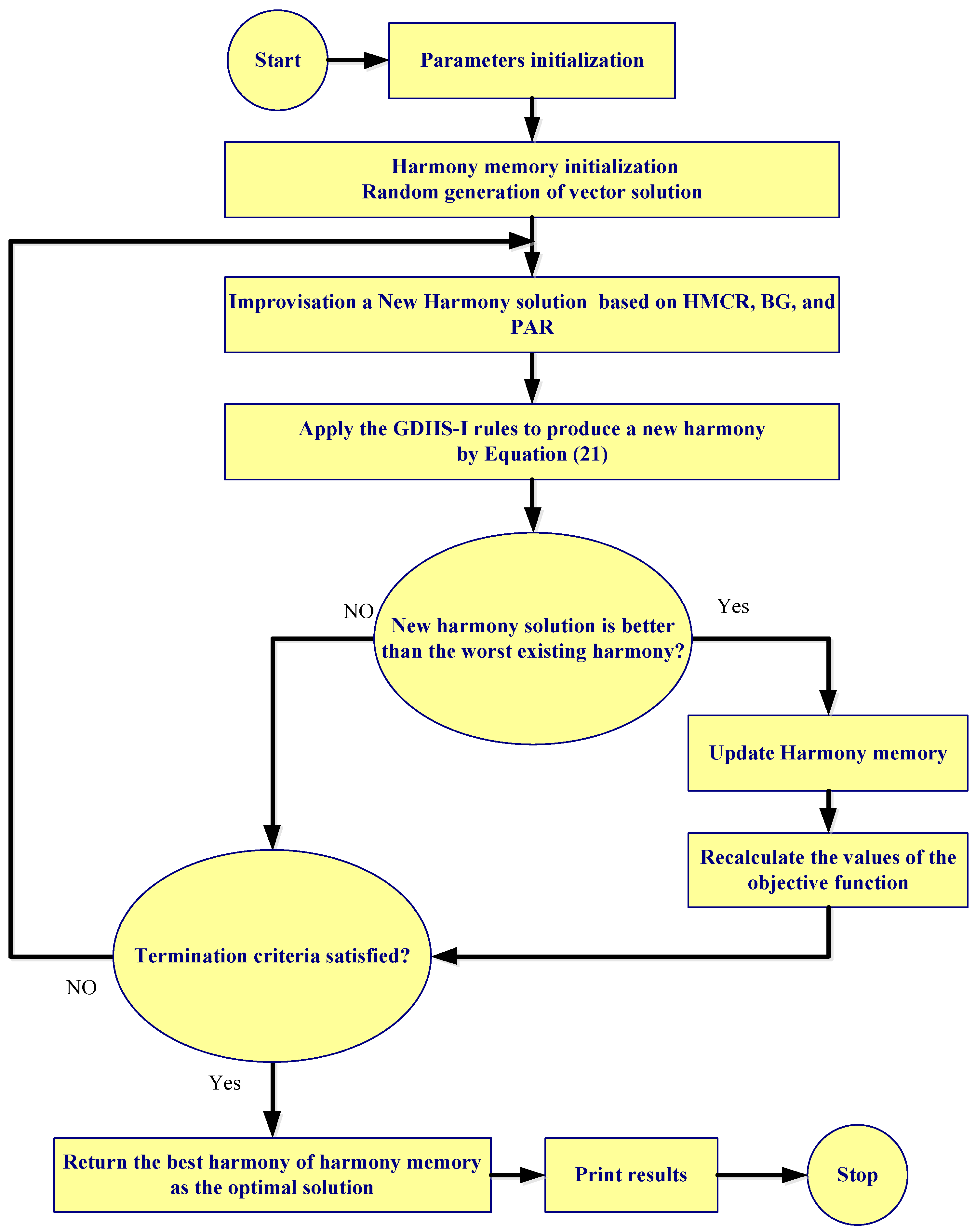
However, the above research uses different optimization algorithms and shows that the HS method is promising for the optimization of the hybrid system but does not use the global dynamic HS method. In this regard, the HS method has disadvantages, including the local optima problem (or becoming stuck in local optima), that have not been addressed. In optimization problems, the local optima are defined as the relative best solutions within a neighbor solution set. Different hybrid solar systems are optimized to meet the load, but the reliability is poor. In addition, the effect of the type of solar panel is not considered in the optimization, and the effects of the initial costs and efficiency of monocrystalline and polycrystalline solar panels are not extracted for the optimization of hybrid systems. Based on the above analysis, in order to identify cost-effective, safe, and reliable operation of power generation systems in remote areas, this paper proposes a new global dynamic harmony search (GDHS-I) algorithm as an optimization algorithm for the optimal sizing of a hybrid photovoltaic–battery scheme. The hybrid photovoltaic–battery scheme is optimized based on different types of solar panels (monocrystalline and polycrystalline). In this regard, the performance optimizations are performed with the original GDHS, original HS, and simulated annealing (SA) to determine the effectiveness of the GDHS-I algorithm. Finally, the effect of initial costs and the efficiency of monocrystalline and polycrystalline solar panels on the optimization of hybrid systems is analyzed. The main contributions of this study in analyzing the performance of hybrid photovoltaic–battery scheme are as follows:

• Introducing a global dynamic harmony search method to perform optimization and to determine the optimal sizing of a hybrid photovoltaic–battery system;
• To determine the effectiveness of the suggested optimization method, the performance optimizations are performed with original global dynamic harmony search, original harmony search, and simulated annealing;
• Based on indicators such as minimizing total cost and loss of load supply probability, the features of the solar panels on the optimal sizing of the hybrid scheme are investigated to determine the best solar panel subsystem selection;
• Sensitivity analysis is conducted on the optimized hybrid systems to test the influence of various initial costs and efficiency of monocrystalline and polycrystalline solar panels.

In the next section, the modeling of the hybrid photovoltaic–battery scheme is given. In Section 3, the objective function is presented. Section 4 gives a detailed methodology of this study. Section 5 illustrates the results and discussion. Section 5 is the conclusion of this article.

2. Modeling of the Hybrid Photovoltaic–Battery Scheme

In this study, optimal sizing of the hybrid photovoltaic–battery scheme to the cost-effective, safe, and reliable operation of power generation systems in remote areas is considered. Figure 1 shows the general configuration of the hybrid PV–battery scheme. Different types of PV panels and batteries are connected through a DC bus, whereas the load is connected through an AC bus in this planning. The produced power from the hybrid photovoltaic–battery system is converted through DC/AC inverter to meet the load demand.

2.1. Photovoltaic

The generated power of the PV array (p_PV) based on solar radiation on a tilted plane module R_t (in kW/m²), the efficiency of the PV panels, and the cell temperature Te_c (°C) can be determined according to the following equations [36,37]:

$$p_{PV}(t)=R_t{\eta }_{PV}{A}_{PV}$$

(1)

$${\eta }_{PV}={\eta }_r{\eta }_{pc}\left[1-N_{Te}\left(T{e}_c-T{e}_{ref}\right)\right]$$

(2)

$$T{e}_c=T{e}_{air}+\left[\frac{NOCT-20}{800}\right]R_t$$

(3)

where A_PV denotes the area of the PV panels (in m²), η_r and η_pc denote the reference module efficiency and the power conditioning efficiency, respectively, Te_ref and Te_air refer to the cell temperature at the reference conditions and ambient air temperature, N_Te is the panel temperature coefficient, and NOCT is the nominal cell operating temperature, which is measured under 20 °C of ambient temperature, 1 m/s wind speed, and 800 W/m² of solar radiation.

2.2. Storage System

The hybrid power generation system based on PV panels needs storage units as a back-up system to supply the electrical demand at lacking PV power generation times. The energy storage level (ESL) of the battery unit is acquired as follows [38,39]:

In charging mode:

$$ESL(t)=ESL(t-1)\cdot \left(1-\sigma \right)+\left[\left(E_{PV}(t)\cdot {\eta }_{INV}\right)-\frac{E_{Load}(t)}{{\eta }_{INV}}\right]\cdot {\eta }_{BC}$$

(4)

In discharging mode:

$$ESL(t)=ESL(t-1)\cdot \left(1-\sigma \right)-\left[\frac{E_{Load}(t)}{{\eta }_{INV}}-\left(E_{PV}(t)\cdot {\eta }_{INV}\right)\right]/{\eta }_{BDC}$$

(5)

where $\sigma$ denotes the rate of hourly self-discharge; η_INV, η_BC, and η_BDC are the efficiency of the inverter, charging, and discharging modes, respectively; and E_Load represents the demand of load at time t (1 h).

3. Objective Function

The considered objective function in the current paper is the total net annual cost (TNAC) minimization based on the loss of load supply probability (LLSP) as a reliability index to find the ideal sizing of the hybrid photovoltaic–battery scheme.

3.1. LLSP

To have an organization with acceptable reliability, LLSP is applied, which shows how often the hybrid photovoltaic–battery scheme is inefficient in meeting the load demand [40,41,42]. The following equation is used for finding LLSP for one year (8760 h):

$$LLSP=\frac{{\displaystyle \sum _{t=1}^{t=8760}LLS(t)}}{{\displaystyle \sum _{t=1}^{t=8760}{E}_{Load}(t)}}$$

(6)

Here, LLS denotes the loss of load supply whenever the energy demand is more than the energy produced (E_Gen):

$$LLS(t)=E_{Load}(t)-E_{Gen}(t)$$

(7)

3.2. TNAC

TNAC includes the annual operation and maintenance cost (O&M) and annual capital and replacement cost (C&R). In the optimization process, the TNAC must be minimized as an objective function:

$$Minimize.TNAC=\sum C\&R+O\&M$$

(8)

By recognizing the project lifetime, replacement periods, annualized O&M costs, and annualized C&R costs for each component of the hybrid photovoltaic–battery system, the TNAC value can be determined according to the following equations:

$$C\&R=CRF\cdot \left[A_{PV}\cdot C\&R_{PV}+N_{BS}\cdot C\&R_{BS}+N_{INV}\cdot C\&R_{INV}\right]$$

(9)

$$O\&M=A_{PV}\cdot O\&M_{PV}+N_{BS}\cdot O\&M_{BS}+N_{INV}\cdot O\&M_{INV}$$

(10)

where N_INV and N_BS denotes the number of inverter and battery, C&R_PV is the PV panel unit cost, C&R_BS is the present worth of battery based on life span of battery (here, 5 years), C&R_INV is the present worth of converter/inverter based on its life span (here 10 years), O&M_PV, O&M_BS, O&M_INV denote the O&M costs of the PV panel, battery, and inverter/converter unit, respectively, and CRF represents the capital recovery factor, which is defined by the following equation based on the interest rate (i) and project life span (n) [43]:

$$CRF=\frac{i{\left(1+i\right)}^n}{{\left(1+i\right)}^n-1}$$

(11)

3.3. Constraints

The optimization algorithm is working according to the highest allowable value of LLSP (here, 2%) [40,41,42] and other limitations of the decision variables (area of the PV panel and number battery):

$$LLSP\le 2\%$$

(12)

$$0\le A_{PV}\le A_{PV-Max}$$

(13)

$$0\le N_{BS}\le N_{BS-Max}$$

(14)

$$ES{L}_{Min}\le ESL\le ES{L}_{Max}$$

(15)

$$ES{L}_{Min}=(1-DOD)\cdot S_{BS}$$

(16)

where N_BS-Max and A_PV-Max refer to the maximum area of the PV panels and the maximum number of batteries, respectively, ESL_Min and ESL_Max are the minimum and maximum energy storage levels of the battery bank, respectively, and S_BA and DOD are the nominal capacity of battery and depth of discharge, respectively.

3.4. Operation Strategy

The operation strategy used in the proposed hybrid photovoltaic–battery system is presented in Figure 2. So, the calculation of the total power production by PV panels and the calculation of the energy storage in storage units as a back-up system to supply the electrical demand at lacking PV power generation times is performed through the loop below during a year (8760 h). Here, j is the number of the configuration of the hybrid system, which is determined based on the maximum number of PV panels, batteries, and the maximum number of iterations in the optimization algorithm.

4. Methodology

Considering the discrete (integer) and continuous nature of decision variables in a size optimization problem, an efficient search technique based on the Harmony Search (HS) is implemented to solve this type of sizing problem.

4.1. Harmony Search (HS)

The HS is an optimization algorithm suggested by Geem et al. [44] in 2001. In this regard, discrete HS, which was proposed by Maleki et al. [45], tends to result in more accurate results when compared with discrete simulated annealing. Harmoney Memory Considering Rate (HMCR), pitch adjustment rate (PAR), and bandwidth of generation (BG) are parameters that are pivotal in the converging process of the aforementioned HS method. These parameters are critically important in providing the algorithm with an optimal solution and speed at which this solution is obtained. The rate at which a value is selected from the Harmony Memory varies between 0 and 1 and is called HMCR. Memory consisting of N_h harmonies is called Harmony Memory. A trial-and-error process was utilized to determine the algorithm parameters, and PAR, HMCR, and BG of the HS algorithm in this process were set to 0.3, 0.9, and 0.03, respectively.

Below are the steps required to generate a new harmony via HS:

Step 1: A uniformly distributed random number is generated between 0 and 1. If the aforementioned number has a greater value than HMCR, the production of the improvised note is going to be random and from the possible range. In addition, the following note is going to be improvised, if not, proceed to Step 2.

Step 2: The value corresponding to the improvised note is a randomly selected note from the pool of HM. The next step is the generation of a uniformly distributed number between 0 and 1. If the value of the aforementioned number is greater than PAR, no change to the value of the improvised note is required. If not, proceed to the third step.

Step 3: If the value of the improvised note is changed by BG, we move to a randomly selected direction via BG value.

If the quality of the newly generated harmony is higher than the worst HM harmony, the newly generated harmony is going to be stored while the worst harmony is removed from HM. This process continues to the point in which the maximum number of iterations is reached.

4.2. Global Dynamic Harmonic Search Algorithm: GDHS

In a recent study, a new HS algorithm was modified by Khalili [46], which was named GDHS. In this modified version of the algorithm, BG, PAR, and HMCR were adjusted via a dynamic approach. Furthermore, in the aforementioned method, the domain changed dynamically, a dynamic mode was introduced for all key parameters, and predefining the parameters was unnecessary. BG, PAR, and HMCR were mathematically expressed via the following formulas:

$$BG\left(t\right)=B{G}_{\max }{\mathrm{e}}^{\left(\frac{Ln\left(\raisebox{1ex}{$B{G}_{\min }$}\!\left/ \!\raisebox{-1ex}{$B{G}_{\max }$}\right.\right)}{ite{r}_{\max }}\times iter\right)}$$

(17)

$$HMCR\left(t\right)=0.9+0.2\times \sqrt{\frac{iter-1}{ite{r}_{\max }-1}\times \left(1-\frac{iter-1}{ite{r}_{\max }-1}\right)}$$

(18)

$$PAR\left(t\right)=0.85+0.3\times \sqrt{\frac{iter-1}{ite{r}_{\max }-1}\times \left(1-\frac{iter-1}{ite{r}_{\max }-1}\right)}$$

(19)

In the above correlations, iter_max stands for the maximum number of iterations, iter indicates the current iteration, and BG_min and BG_max are the symbolic representations of the minimum and the maximum band with values, respectively.

New Harmony is found by applying the following relation:

$$x_{new,j}=x_{new,j}+BG\times \left(rand-0.5\right)\cdot \left(x_{best,j}-x_{new,j}\right)$$

(20)

4.3. GDHS-I

Considering the prevention of local optima, this section is dedicated to introducing the newly developed GDHS algorithms incorporating the pitch adjustment mechanism, namely, the GDHS-I algorithm. New Harmony is found by applying the following relation:

$$x_{new,j}=x_{new,j}+rand\times \cdot \alpha \cdot \left(x_{best,j}-x_{new,j}\right)$$

(21)

In the aforementioned formula, $\alpha$ represents the weighting factor, which is selected based on hybrid system components, where x_best shows the best harmony.

Figure 3 is a representation of the computational procedure in this novel GDHS algorithm.

5. Results and Discussion

In this section, the results obtained by applying the suggested optimization algorithm (new global dynamic harmony search (GDHS-I)) to the hybrid photovoltaic–battery system will be presented. Furthermore, performance optimizations are performed with the original GDHS [47], original HS [48], and simulated annealing [49] to determine the effectiveness of the GDHS-I method. MATLAB software is used to implement the suggested optimization methods on a computer PC (core-i7, 6 GB RAM, and 2.3 GHz CPU). The used optimization model is measured to achieve a case study in Rafsanjan (30°24′24″ N 55°59′38″ E), Iran. For this purpose, the parameters of the stand-alone hybrid system are presented in

Table 1. Parameters of the hybrid system components.

Economic
r	10%
n	20 years
PV Panel
Life Span	25
C&RPV (Mono-SI)	210 USD/m2
C&RPV (Poly-SI)	120 USD/m2
O&MPV	2% CPV USD/m2/year
Efficiency (Mono-SI)	20%
Efficiency (Poly-SI)	15%
Battery
SBA	2.1 kWh
ηBC	85%
PBS	USD 310
Life span	5 years
DOD	80%
ω	0.02%
O&MBS	10 USD/year
Converter/Inverter
Rated power	3 kW
ηINV	95%
Life span	10 years
PINV	USD 1583
O&MINV	15 USD/year

, and the parameters of the optimization algorithms are given in

Table 2. Parameters of the optimization algorithms.

Harmony Search (HS)		Global Dynamic HS (GDHS)		GDHS-I		SA
HMCR	0.9	BGmax	1	BGmax	1	Step size	0.97
PAR	0.3	BGmin	0.01	BGmin	0.01	Initial temperature	100
BG	0.03	itermax	2000	α	2	itermax	2000
itermax	2000			itermax	2000

[37,50,51,52,53]. In addition, the typical load demand, solar insolation, and ambient temperature during a year (8760 h) are used in this study, which are given in Figure 4.

As the harmony search method uses stochastic random searches in the search space, various runs may lead to finding various solutions. To solve this problem, the optimal solution is reported after several runs. In this regard, 30 independent runs for each algorithm (HS, GDHS, SA, and GDHS-I) are executed to provide valid results, and the optimal results are determined. These results for two types of solar panels (Poly-SI and Mono-SI) are reported in

Table 3. Results found by the studied algorithms for two types of solar panels.

Types of Solar Panels	Algorithms\Index	Best (USD)	Worst (USD)	Mean (USD)	Std. (USD)	Mean Time (s)
Poly-SI	HS	112,175	304,111	177,743	50,614	5.8604
	GDHS	109,907	260,735	160,051	33,593	5.8292
	GDHS-I	103,777	196,069	122,287	19,314	5.7495
	SA	223,570	1,795,007	1,142,542	439,224	13.6854
Mono-SI	HS	111,413	353,070	201,940	66,671	5.7229
	GDHS	105,580	291,204	162,397	49,245	5.7057
	GDHS-I	104,686	198,360	129,355	22,191	5.6776
	SA	138,654	1,783,164	1,161,845	417,844	14.3161

, which includes the average, worst (maximum), best (minimum), and standard deviation (Std.) of the TNAC value and the average simulation time indices.

The optimization method is aimed at minimizing the TNAC value and the loss of load supply probability of the hybrid photovoltaic–battery system based on the optimum number of battery banks and area of the PV panels. The minimum bound of the battery banks and the area of the PV panels are set to 0, and the maximum bound of the battery banks and the area of the PV panels are set to 20,000 and 350 m², respectively. In Poly-SI solar panels, the best fitness function value of the photovoltaic–battery system is USD 103,777, which is obtained by the GDHS-I algorithm. The subsequent ranks are displayed by GDHS, HS, and SA respectively. When utilizing the GDHS, HS, and SA methods, the minimum TNAC of the studied system is found to be USD 109,907, USD 112,175, and USD 223,570, respectively. The relative error between the Best index of the GDHS-I and GDHS, $\left|\frac{Bes{t}_{GDHS-I}-Bes{t}_{GDHS}}{Bes{t}_{GDHS-I}}\right|\times 100$, is 5.9%, and between the Best index of the GDHS-I and HS, it is 8.1%. In addition, the relative error between the Mean index of GDHS-I and GDHS is 30.9%, and between the Mean index of the GDHS-I and HS, it is 45.3%. The best average simulation time value of the system is 5.7495 s, which is obtained by the GDHS-I algorithm. The worst average simulation time value of the system is 13.6854 s, which is obtained by the SA algorithm. Based on the mean and average simulation time indices, the result shows that the GDHS-I is better than the GDHS, HS, and SA methods (Figure 5). As a result, based on different indices (Best, Worst, Mean, Std., and Meantime), the GDHS-I method has more stoutness that the GDHS, HS, and SA methods, respectively. The convergence characteristics of the GDHS-I, GDHS, HS, and SA algorithms for Poly-SI solar panels are presented in Figure 6, which shows the superiority of GDHS-I in finding the best fitness function value.

In Mono-SI solar panels, the minimal TLCC, which denotes the optimal setup, is USD 104,686, which is found by the GDHS-I algorithm. The subsequent ranks are displayed by GDHS (USD 105,580), HS (USD 111,413), and SA (USD 138,654), respectively. The relative error between the Best index of the GDHS-I and GDHS is 0.9%; between the Best index of the GDHS-I and HS it is 6.4%; and between the Best index of the GDHS-I and SA it is 32.45%. In this case, the Mean, Worst, and Std. values of the fitness function are USD 129,355, USD 198,360, and USD 22,191, respectively, which are obtained by the GDHS-I algorithm. In this regard, the relative error between the Mean index of GDHS-I and GDHS is 25.5%, and between the Mean index of the GDHS-I and HS it is 56.1%. The mean simulation time value of the system is 5.6776 s, which is obtained by the GDHS-I algorithm. The mean simulation time and the mean fitness function values with the proposed algorithms for Mono-SI solar panel are shown in Figure 7, which shows the superiority of GDHS-I based on the mean simulation time and the mean fitness function values. Figure 8 shows the convergence characteristic of the GDHS-I, GDHS, HS, and SA algorithms for the Mono-SI solar panels. It can be seen that the GDHS-I method is better than other methods in finding the best fitness function value.

To ensure the reliability of the GDHS-I method, the performance of the GDHS-I method is compared after the different number of runs (30 to 200) for two types of solar panels. The results found by the GDHS-I algorithm for the two types of solar panels for the different number of runs are presented in

Table 4. Results found by the GDHS-I algorithm for two types of solar panels for different number of runs.

Types of Solar Panels	Number of Runs	Best (USD)	Worst (USD)	Mean (USD)	Std. (USD)
Poly-SI	30	103,777	196,069	122,287	19,314
	40	103,777	161,764	119,379	13,304
	60	103,777	181,220	122,613	15,539
	100	103,777	162,999	119,525	12,029
	150	103,777	181,774	119,353	12,808
	200	103,777	210,169	119,495	13,921
Mono-SI	30	104,686	198,360	129,355	22,191
	40	104,686	170,772	122,140	14,352
	60	104,686	157,520	121,631	11,673
	100	104,686	184,150	121,195	14,619
	150	104,686	183,086	122,911	13,280
	200	104,686	171,510	121,221	13,081

. In this Table, the effect of the number of runs on the optimal system is investigated. In Poly-SI solar panels, when the number of runs is equal to 30, the best fitness function value of the photovoltaic–battery system is USD103,777, which is similar to that found with 40 to 200 independent runs. In the Mono-SI Solar Panel, when the number of runs is equal to 30, the minimum TNAC of the studied system is USD 104,686. When the number of runs is equal to 30 to 200, the minimum TNAC of the studied system (Best index) is the same.

The optimal configurations of the hybrid photovoltaic–battery scheme for different types of solar panels (Poly-SI and Mono-SI) by the proposed algorithms are reported in

Table 5. Optimal configurations of the hybrid photovoltaic–battery scheme for different types of solar panels.

Types of Solar Panels	Algorithms\Index	APV (m2)	NBS	TNAC (USD)	LLSP (%)
Poly-SI	HS	149.2	1179	112,175	1.5612
	GDHS	146.2	1155	109,907	1.9824
	GDHS-I	147	1088	103,777	1.9644
	SA	139.4	2395	223,570	1.7805
Mono-SI	HS	109.9	1166	111,380	1.9241
	GDHS	110.2	1103	105,609	1.9523
	GDHS-I	110.1	1093	104,686	1.9924
	SA	107.5	1465	138,654	1.9314

. In Poly-SI solar panel, the optimal number of battery storage, and area of the PV panels, TNAC, and LLSP, found by GDHS-I, are 1088, 147 m², USD103,777, and 1.9644%, respectively. It is observed that when using GDHS, the values of TNAC and LLSP increase to USD109,907 and 1.9824%, respectively. It can be seen that the values A_PV and N_BS are 146.2 m² and 1155 in this case. When the HS algorithm is used, the optimal number of battery storage, and area of the PV panels, TNAC, and LLSP are 1179, 149.2 m², USD112,175, and 1.5612%, respectively. Also, when the SA algorithm is used, the optimal number of battery storage, and area of the PV panels, TNAC, and LLSP are 2395, 139.4 m², USD223,570, and 1.7805%, respectively. The TNAC and LLSP values with GDHS-I, GDHS, HS, and SA algorithms for Poly-SI solar panels are shown in Figure 9. Among the results of the four algorithms, it is observed that the optimal configurations of the hybrid photovoltaic–battery scheme with the lowest cost (USD103,777) and appropriate reliability are obtained by the GDHS-I algorithm. In this regard, in the highest allowable value of LLSP (here 2%), the GDHS-I shows approximately 5.6% & 7.5% cost saving in comparison with the GDHS & HS, respectively. Also, the GDHS-I shows approximately USD 119,793 cost saving in comparison with the SA algorithm.

In Mono-SI solar panel, the optimal values of A_PV, N_BS, TNAC, and LLSP are 110.1 m², 1093, USD104,686, and 1.9924%, respectively. They are found by the GDHS-I algorithm. Also, shows that the values of A_PV, N_BS, TNAC, and LLSP of the hybrid system are 110.2 m², 1103, USD105,609, and 1.9523%, respectively by the GDHS algorithm. In this case, the optimal values of A_PV and N_BS are 109.9 m² and 1166, respectively, by the HS algorithm. When the SA algorithm is used, the optimal values of A_PV, N_BS, TNAC, and LLSP of the hybrid system are 107.5 m², 1465, USD138,654, and 1.9314%, respectively. The TNAC and LLSP values with suggested algorithms for Mono-SI solar panel are shown in Figure 10. It can be seen that the GDHS-I algorithm with the lowest cost (USD 104,686) and appropriate reliability has superior robustness to the GDHS, HS, and SA methods due to its optimal values for the TNAC and LLSP. In this regard, in the highest allowable value of LLSP (here 2%), the GDHS-I shows approximately USD 923, USD 6694, and USD 33,968 cost savings in comparison with the GDHS, HS, and SA, respectively.

Sensitivity Analysis

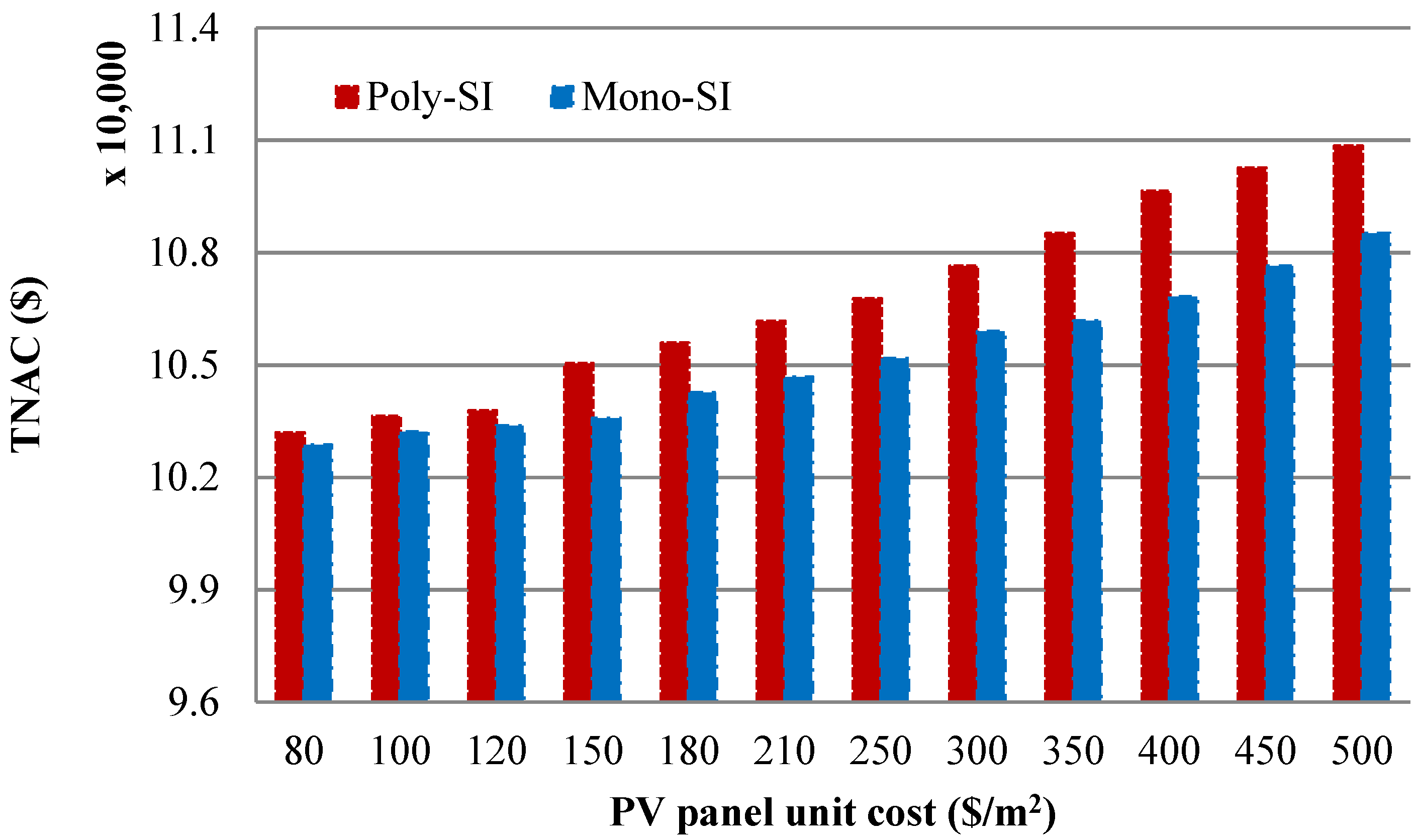
In this section, first, the effect of the PV panel unit cost on the optimal system is investigated, and then the effect of the PV panel efficiency on the optimal hybrid system is analyzed. The optimal configurations of the hybrid photovoltaic–battery system for different types of solar panels for different PV panel unit costs are reported in

Table 6. The optimal configuration of the hybrid photovoltaic–battery scheme for different types of solar panels for different PV panel unit cost.

	Mono-SI Solar Panel				Poly-SI Solar Panel
PV Panel Unit Cost (USD/m2)	APV (m2)	NBS	TNAC (USD)	LLSP (%)	APV (m2)	NBS	TNAC (USD)	LLSP (%)
80	110.2	1092	102,862	1.9607	146.9	1089	103,192	1.9796
100	110.6	1093	103,219	1.9014	146.9	1090	103,630	1.9722
120	111	1092	103,384	1.8342	147	1088	103,777	1.9644
150	110.3	1090	103,586	1.9523	147.1	1096	105,047	1.9502
180	110.7	1093	104,261	1.8877	147.6	1096	105,580	1.8811
210	110.1	1093	104,686	1.9924	147.4	1096	106,167	1.9078
250	110.5	1093	105,166	1.9068	147	1096	106,772	1.9543
300	110.1	1094	105,889	1.9774	147.1	1096	107,637	1.9502
350	110.2	1090	106,173	1.9687	147.2	1096	108,509	1.9296
400	110.6	1090	106,823	1.9605	147.1	1099	109,639	1.9464
450	110.1	1092	107,642	1.9909	147.5	1096	110,255	1.8914
500	110.7	1094	108,515	1.8782	147.4	1093	110,841	1.9034

. In Mono-SI solar panels, when the PV panel cost is equal to 210 USD/m², the optimal values of the TNAC and LLSP of the hybrid scheme are USD 104,686 and 1.9924%, respectively. In addition, the values of A_PV and N_BS are 110.1 m² and 1093, respectively. When the PV panel cost is equal to 150 USD/m² and 300 USD/m², the optimal values of the TNACs of the hybrid system are USD 103,586 and USD 105,889, respectively. It is observed that by reducing the PV cost from 210 USD/m² to 150 USD/m², the value of the TNAC decreases to 1.1%, and by increasing the PV cost from 210 USD/m² to 300 USD/m², the value of the TNAC increases to 1.2%. In Poly-SI solar panels, when the PV panel cost is equal to 210 USD/m², the optimal values of the TNAC and LLSP of the hybrid system are USD 106,167 and 1.9078%, respectively. In addition, the values of A_PV and N_BS are 147.41m² and 1096, respectively. It is observed that by reducing the PV cost from 210 USD/m² to 150 USD/m², the value of TNAC decreases to USD 1120, and by increasing PV cost from 210 USD/m² to 300 USD/m², the value of TNAC increases to USD1470. As a result, by increasing the Mono-SI solar panel and Poly-SI solar panel unit costs, the TNAC of the hybrid system is increased (Figure 11). A comparison between the Mono-SI and Poly-SI solar panels shows that, at the same cost, the optimal values of A_PV and TNAC of the hybrid system based on Poly-SI solar panels is more than the hybrid system based on Mono-SI solar panels. In other words, the hybrid system based on Mono-SI solar panels shows about a 37% A_PV saving in comparison with the hybrid system based on Poly-SI solar panels. In addition, the hybrid system based on Mono-SI solar panels shows about 1.5% cost savings in comparison with the hybrid system based on Poly-SI solar panels. The reason for the difference in cost, despite the same cost, is the difference in efficiency between the two panels.

The optimal configurations of the hybrid photovoltaic–battery system for Mono-SI solar panels based on different PV efficiency are reported in

Table 7. The optimal configuration of the hybrid photovoltaic–battery scheme for Mono-SI solar panel based on different PV efficiency.

PV Efficiency (%)	APV (m2)	NBS	TNAC (USD)	LLSP (%)
16.5	133.8	1094	105,545	1.9354
18	122.6	1095	105,277	1.9350
20	110.1	1093	104,686	1.9924
22	100.1	1074	102,619	1.9999
24	91.8	1073	102,261	1.9990

. In PV efficiency equal to 20%, the optimal values of A_PV, N_BS, TNAC, and LLSP of the hybrid system are 110.1 m², 1093, USD 104,686, and 1.9924%, respectively. In the PV efficiency equal to 16.5%, the optimal values of TNAC, A_PV, N_BS, and LLSP of the hybrid system are USD 105,545, 133.8 m², 1094, and 1.9354%, respectively. 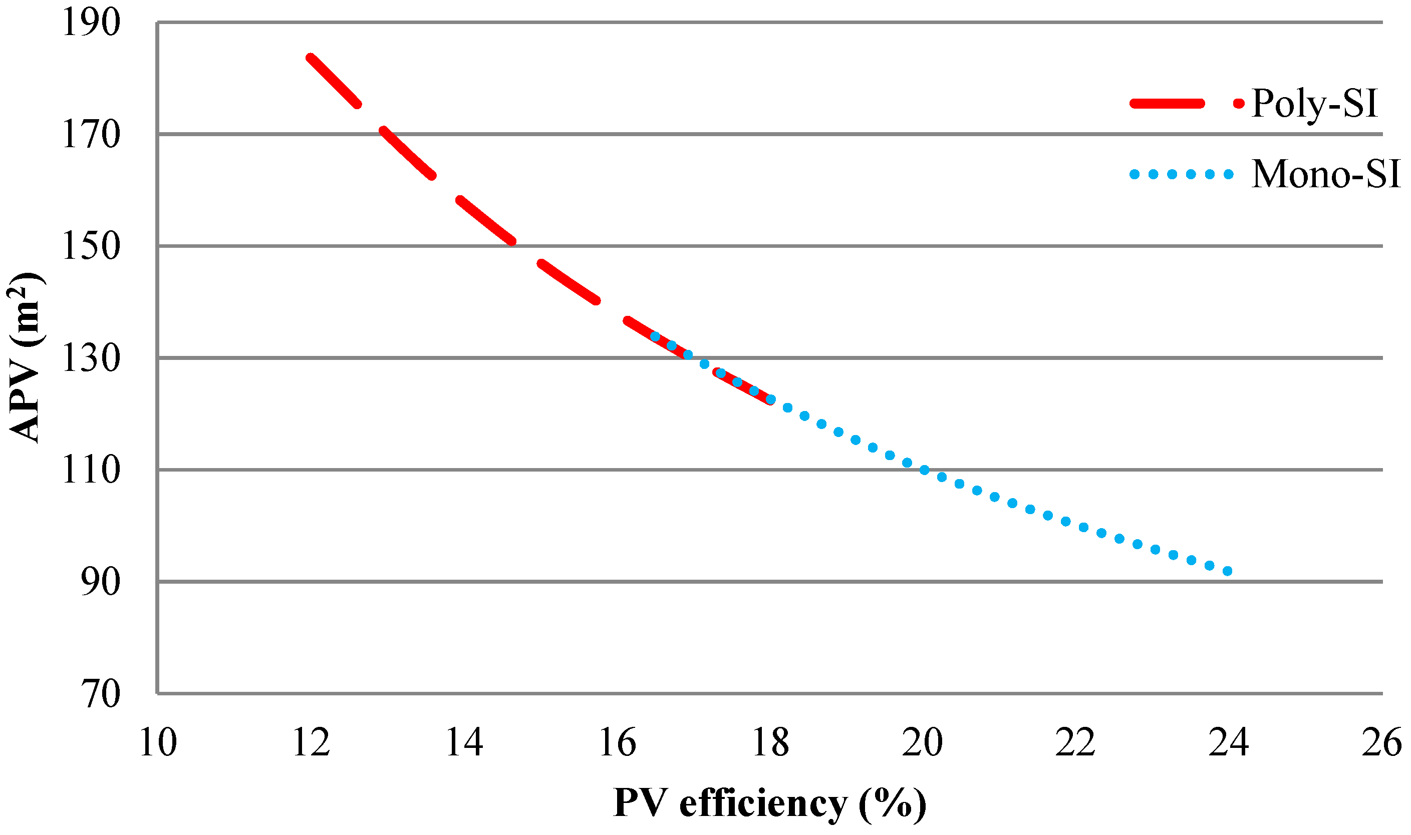It is observed that by reducing PV efficiency from 20% to 16.5%, the value of TNAC and A_PV increase to USD 859 and 21.5%, respectively, and by increasing the PV efficiency from 20% to 24%, the value of TNAC, A_PV, and N_BS decrease to 2.3%, 16.6%, and 1.8%, respectively. The optimal areas of the PV panel of the hybrid scheme vs. PV efficiency in the optimal situation for the Mono-SI solar panel are presented in Figure 12. It is observed that by increasing the PV efficiency from 16.5% to 24%, the optimal value of A_PV is decreased from 133.8 m² to 91.8 m².

The optimal configurations of the hybrid photovoltaic–battery system for Poly-SI solar panels based on different PV efficiencies are presented in

Table 8. The optimal configuration of the hybrid photovoltaic–battery scheme for Poly-SI solar panel based on different PV efficiency.

PV Efficiency (%)	APV (m2)	NBS	TNAC (USD)	LLSP (%)
12	183.6	1108	106,386	1.9514
13.5	163.5	1104	105,595	1.9191
15	147	1088	103,777	1.9644
16.5	133.66	1087	103,403	1.9624
18	122.4	1077	102,247	1.9972

. In PV panel efficiencies equal to 15%, the optimal values of TNAC and LLSP of the hybrid system are USD 103,777 and 1.9644%, respectively. In addition, the optimal values of A_PV and N_BS are 147 m² and 1088, respectively. In the PV efficiency equal to 12% and 18%, the optimal value of the TNAC of the hybrid system is USD 106,386and USD 102,247, respectively. It is found that by reducing PV efficiency from 15% to 12%, the value of TNAC increases to 2.5%, and by increasing the PV efficiency from 15 to 18%, the value of TNAC decreases to 1.5%. Figure 12 shows the area of the PV panel of the hybrid scheme vs. PV efficiency in the optimal condition for the Poly-SI solar panel. It is found that by reducing PV efficiency from 18% to 12%, the value of A_PV is increased from 122.4 m² to 183.6 m².

6. Conclusions

In this study, a new optimization approach, global dynamic harmony search, is presented for optimal sizing of a hybrid photovoltaic–battery scheme to find minimum cost and reliable supply of electricity. The optimal sizing of the stand-alone hybrid scheme is determined by applying two types of PV panels (monocrystalline and polycrystalline). The performance optimizations by the proposed algorithm are compared with the original global dynamic harmony search, original harmony search, and simulated annealing to determine the effectiveness of the suggested optimization method. The effect of initial costs and efficiency of monocrystalline and polycrystalline solar panels on the optimization of hybrid systems is analyzed. The results show that, based on different indices (Best, Worst, Mean, Std., and Meantime), the GDHS-I algorithm has superior robustness to the GDHS, HS, and SA methods due to its optimal values for the TNAC and LLSP. As a result, by increasing the Mono-SI solar panel and Poly-SI solar panel unit costs, the TNAC of the hybrid system are increased. In addition, by increasing Poly-SI solar panel efficiency from 12% to 18%, the optimal values of PV areas and the amount of battery storage decrease to 3.9% and 2.8%, respectively. Moreover, by increasing Mono-SI solar panel efficiency from 16.5% to 24%, the optimal value of PV areas and the amount of battery storage decreases to 3.1% and 2%, respectively.