1. Introduction
World trade has maintained a growth trend since the 21st century. The World Trade Organization [
1] reported that trade in goods expanded by 4.6% on average between 2005 and 2017, which enables the continuous growth of transportation demand. China’s “One Belt One Road” initiative promotes world trade development and creates higher requirements for transportation infrastructure.
Container transportation is an advanced transportation mode in the modern transportation industry, which is an important tool to realize multimodal transportation and to complete commodity transportation and delivery for world trade efficiently and safely. Maritime transportation systems are important infrastructures to enable transportation activities [
2]. This study focuses on a crucial subsystem of maritime transportation systems called the “port–hinterland container logistics transportation system” (PHCLTS). It is the landside component of maritime transportation systems [
3], which realizes container transportation between a port and its hinterlands to support the national economy and people’s lives.
A PHCLTS is an extremely complex transportation system that contains diverse infrastructures, transportation modes, and participants.
Figure 1 shows the infrastructure structure of a PHCLTS, and it is composed of several nodes and arcs. The nodes of the PHCLTS represent a port, several multimodal connection points, and numerous hinterland points. Only one port exists in a PHCLTS, and the port is an important hub connecting maritime process and port–hinterland transportation process. The transportation mode of containers can be changed at the multimodal connection points, including multimodal terminals, dry ports, and inland ports. The hinterland points correspond to the demand and supply areas, including warehouses, distribution centers, and factories. The arcs of the PHCLTS represent roads, railways, and inland rivers, which connect the different nodes of the PHCLTS. A PHCLTS contains diverse transportation modes, including road, rail, inland river, and multimodal transportation. It also contains diverse participants, such as the government, shippers, port companies, truck carriers, rail carriers, inland-river carriers, and logistics service providers.
However, various kinds of unconventional emergency events (UEEs), such as natural or human-caused disasters, threaten PHCLTSs. Consequently, the performance of PHCLTSs will decline and exert negative effects on the economy and society. For example, in August 2005, the United States of America was hit by Hurricane Katrina, which stopped the operation of highway and railway trunk lines between the Port of New Orleans and its hinterland. The supply chains of many industries were interrupted because of the severe damage in infrastructure, people’s lives and the production processes of enterprises were affected, and the economic growth rate of the United States of America slowed down.
Improving the recovery capability of PHCLTSs in the face of UEEs is critical. The concept of “resilience” is applied to describe such a capability; this concept refers to the capacity of a logistics transportation system to recover to an acceptable operational service level after being affected by a disruption, and the level of efforts under resource restrictions, such as immediate recovery activities implemented in the logistics transportation system, should be considered when measuring the resilience of the logistics transportation system [
4]. This study aims to provide an optimal decision-making reference for governments to improve the resilience of PHCLTSs in the face of UEEs to recover the operational capacity efficiently and reduce the negative effects of UEEs.
Logistics transportation system participants, including organizations and individuals, will affect the resilience of the system through their actions and interactions [
5]. To study the resilience problem of PHCLTSs, the behaviors and interactions of associated participants should be analyzed.
Therefore, a bi-level programming model consisting of two submodels is applied to analyze the resilience problem of PHCLTSs. The upper and lower level models have decision variables, objective functions, and constraints of their own. Furthermore, it contains the hierarchical relationship and interaction between decision makers of the two submodels and can deal well with their two conflicting goals [
6]. For the upper level model, the decision maker is the planner of PHCLTSs, i.e., the government, which as the leader makes decision on immediate recovery activities to improve the resilience of PHCLTSs. For the lower level model, the decision makers are the users of PHCLTSs, i.e., shippers and carriers. The shippers make decisions about the demands for containers in hinterlands, and the carriers complete the actual transportation process of containers in the recovered PHCLTS that are from port to hinterland points in accordance with the shippers’ demand. In this study, truck carriers are selected because road transportation is a critical mode of freight transportation at present. Truck carriers, which are the followers, make decisions about transportation routes and freight volume in the recovered PHCLTS to pursue profit maximization [
7], affecting the achievement of the goal of the government.
The contributions of this paper are the following:
- (1)
Time resilience is adopted to measure and improve the resilience of a PHCLTS with considerations of PHCLTS user behaviors and the hierarchical relationship and interaction of government and truck carriers.
- (2)
Bi-level programming models with two different lower level models are established according to different behavior patterns of PHCLTS users, supporting the government in selecting a reasonable budget level and implementing efficient recovery decisions to aid the PHCLTS to recover the operational capacity in the face of UEEs.
- (3)
It expands the prearranged planning about UEEs and provides a decision-making reference and scientific theoretical support for an efficient response to UEEs.
The remainder of this paper is structured as follows. An overview of the relevant literature is provided in
Section 2. The bi-level programming models with two different lower level models are established in
Section 3. The solution algorithm is constructed in
Section 4. Numerical experiments are conducted to illustrate the validity of the models in
Section 5. Lastly, managerial insights and conclusions are summarized in
Section 6.
2. Literature Review
This study analyzes the resilience problem of PHCLTSs by using the bi-level programming approach. It aims to learn about three aspects from the relevant literature: the resilience of transportation systems corresponding to the goal of the government, logistics transportation system assignment and equilibrium corresponding to the behaviors of PHCLTS users, and the bi-level programming model for logistics transportation system problems corresponding to the approach used in this study.
2.1. Resilience of Transportation Systems
Scholars discussed characteristics of resilient systems and sought to optimize system resilience. Bruneau et al. [
8] defined resilience as the capacity of a system to alleviate the negative influence of a shock, absorb it, and recover promptly after it happens. Murray-Tuite [
9] listed 10 dimensions of transportation resilience and provided several measurement methods for transportation resilience. Ta et al. [
5] discussed the properties of the resilience of a freight transportation system and argued that the resilience is related to physical infrastructure, managing organization, and users. Quantitative studies are conducted on the basis of qualitative studies on this issue. Scholars established mathematical models to measure the resilience of transportation systems while accounting for the limitation of time, cost, and other resources. Omer et al. [
10] defined resilience as the capacity of a maritime transportation system to recover to the normal level in the face of a shock, and tonnage resiliency, time resiliency, and cost resiliency are proposed as metrics. Faturechi and Miller-Hooks [
11] established a bi-level and three-stage stochastic programming model to optimize travel time resilience of passenger transportation systems.
Regarding the resilience of port–hinterland logistics and multimodal transportation systems, Nair et al. [
12] employed resilience as a quantitative measure to determine the optimal actions to enhance security at the nodal facilities of a freight transportation network. Chen and Miller-Hooks [
4] indicated that the level of effort should be considered when measuring the resilience of an intermodal freight transportation system. They proposed an indicator that the system resilience should be equal to the ratio of the transportation demand satisfied post-disaster to the transportation demand satisfied pre-disaster. Subsequently, Miller-Hooks et al. [
13] maximized the resilience of freight transportation networks while considering the implementation of pre-disaster preparation activities and post-disaster recovery activities. Chen et al. [
14] introduced a quantitative method to measure the resilience of a port–hinterland container transportation network from the perspective of shippers. Chen et al. [
3] used the network game theory approach to analyze the strategic investment decision of each participant in a port–hinterland container transportation network to enhance the network’s resilience.
2.2. Logistics Transportation System Assignment and Equilibrium
The behaviors of the transportation system users will affect the transportation system resilience. Existing research on modeling behaviors of logistics transportation system users mostly follows Wardrop’s two principles. Wardrop’s first principle indicates that each transportation system user pursues cost minimization noncooperatively. A “user equilibrium (UE)” assignment in accordance with Wardrop’s first principle occurs when no one in the network can decrease his cost by unilateral action [
15]. Using Wardrop’s first principle, Jones et al. [
16] established an equilibrium model with capacity constraints of links and congestion delays to analyze import and export container flows of the U.S. Meng and Wang [
17] studied the intermodal transportation system design problem with multiple stakeholders and multitype containers by using a mathematical program with an equilibrium constraint model. Corman et al. [
18] proposed an assignment model which can obtain the equilibrium flows and generalized costs to optimize the performance of transportation systems.
Wardrop’s second principle indicates a central authority coordinates all transportation system users to cooperate fully to achieve the total transportation cost minimization of the entire network. A “system optimum (SO)” assignment in accordance with Wardrop’s second principle occurs when the total marginal costs of transportation alternatives are equal [
15]. Using Wardrop’s second principle, Zhang et al. [
19] adopted an SO model to minimize the total cost of a trucking company in the upper level of a bi-level programming model to analyze the urban freight transportation problem. Jiang et al. [
20] established a bi-level programming model to study the design problem of a regional multimodal logistics system with the goal of emission reduction under uncertain demands, and in the lower level model, the carrier arranged the transportation routes for freight demand based on the SO principle to minimize the total generalized transportation cost. Yu and Jiang [
21] constructed a bi-level model to study the logistics transportation system design and delivery scheme problem while adopting an SO model to achieve cost minimization in the lower level model.
2.3. Bi-Level Programming Model for Logistics Transportation System Problems
Research on logistics transportation system optimization that applies a bi-level programming model remains limited. In general, a planning authority in the upper level seeks to maximize the total utility of the entire transportation system. Logistics transportation system users in the lower level determine the transportation process according to the authority’s decision. Moreno-Quintero et al. [
22] established a bi-level programming model to characterize the interaction between the road planner and carriers and studied the road maintenance and overloading control problem. Lee et al. [
23] constructed a bi-level programming model to capture interactions between shippers and different types of carriers in maritime logistics transportation systems. Qiu et al. [
24] employed a bi-level programming model to analyze the carbon emission problem in road freight transportation. Li et al. [
25] used the goal programming approach to study the problem of logistics infrastructure investment and CO
2 emission reduction.
2.4. Summary of Literature Review
“Resilience” is a relatively new concept for logistics transportation systems. Previous research mostly studied the resilience problems of logistics transportation systems from the perspective of demand realization [
4,
12,
13,
14], and such research quantitatively characterized the resilience of logistics transportation systems by using the ratio of the freight demand that can be satisfied post-disaster to the freight demand that can be satisfied pre-disaster. Their perspective focused on measuring and improving the resilience of logistics transportation systems under the following single transportation period after UEEs.
In this study, a medium- and long-term perspective, which focuses on the resilience of logistics transportation systems under multiple transportation periods after UEEs, is applied. The recovered state of a PHCLTS will last for a period of time after the implementation of immediate recovery activities, and the logistics transportation process will be repeated for multiple transportation periods during this time. Hence, time resilience is adopted to measure and improve the resilience of a PHCLTS. It is represented as the ratio of the total transportation time of the PHCLTS in each transportation period pre-disaster to the total transportation time of the PHCLTS in each transportation period post-disaster.
Previous studies rarely considered the hierarchical relationship and interaction among different participants when analyzing the resilience problem of transportation systems. For instance, Faturechi and Miller-Hooks [
11] optimized the travel time resilience of a passenger transportation system while employing a bi-level programming approach to describe the behaviors and interactions of different participants. User behaviors were formulated as a partial user equilibrium in the lower level model. In the current study, the objectives are to explore PHCLTSs, which are freight transportation systems, and to improve the resilience of PHCLTSs, while the hierarchical relationship and interactions among different participants of a PHCLTS are considered. Specifically, two different behavior modes of PHCLTS users are considered on the basis of the SO and UE principles.
Optimization problems of logistics transportation systems have been successfully solved using bi-level programming methods under conventional situations. Nevertheless, research on logistics transportation systems with different decision makers in the face of UEEs is still lacking. This study fills the research gap in this field to analyze how to improve the resilience of PHCLTSs under UEE situations while considering PHCLTS user behaviors, and the hierarchical relationship and interaction of the PHCLTS planner and users. It provides decision support to governments to make highly effective decisions about immediate recovery activities after UEEs, aiding PHCLTSs to recover their operational capacity efficiently.
3. Model
3.1. Model Description and Assumptions
Only one port exists in the targeted PHCLTS. All containers are transported from the port to hinterland points via single mode transportation. The research target is a single-mode PHCLTS, i.e., road transportation by truck carriers. The reason is that road transportation is the critical mode of freight transportation at present. Some PHCLTSs are relatively small in size in the early stage of their development and are connected only by roads. For example, Jones et al. [
16] mentioned that few railway facilities had access to the ports in South Florida at that time, and almost all freight transportation between the ports and hinterlands was realized through road transportation.
The participants of a PHCLTS include the PHCLTS planner and users. The PHCLTS planner is the government, which is the leader and the decision maker in the upper level model. The PHCLTS users include shippers and carriers, which are the followers and decision makers in the lower level model. The decision framework is shown in
Figure 2.
UEEs affect the arcs of PHCLTSs. After the occurrence of a UEE, the government makes decisions on immediate recovery activities for a damaged PHCLTS within the given budget constraint, with the goal of improving the resilience of the PHCLTS. The recovery activities refer to the relevant activities implemented immediately to reduce the negative influence of a UEE and restore the capacity of the PHCLTS. In this study, the recovery activities are filling and repairing the damaged part of an arc to recover a proportion of the transportation capacity of the arc. The recovery activities are implemented only once for each attacked arc in the PHCLTS. The recovery state of the PHCLTS will remain for a period. To complete the recovery activities on each damaged arc efficiently, no limitation is imposed on the implementation time of the recovery activities. The government fully understands the container demands of shippers in the PHCLTS and the behavior modes of truck carriers in the recovered PHCLTS. After the government completes the implementation of recovery activities, the transportation capacity and post-disaster, free-flow travel time of each arc of the recovered PHCLTS will be determined. These two factors will have an influence on truck carriers in arranging the transportation process of containers to achieve the goal of profit maximization.
There are diverse decision makers in the freight transportation process [
26]. The demands for containers in hinterland points are determined by shippers, which is one type of PHCLTS user. Container transportation activities from the port to hinterland points are repeated every day. The daily transportation demands of hinterland points are determined by shippers, which is one type of PHCLTS user, and the container demands are constants and unaffected by UEEs, i.e., the daily transportation demands of hinterland points are regarded as exogenous constants. This assumption has also been adopted in the existing literatures [
14,
18]. Before a UEE happens, all the transportation demands in hinterland points can be satisfied. The sizes of the containers are the same in this study, and all containers are forty-foot equivalent unit (FEU) containers. The value of goods loaded in each container is equal, i.e., the urgency for transporting each container is the same. Each truck transports one FEU container at one time.
Another type of PHCLTS user is truck carriers. The truck carriers fully understand the recovery state of the PHCLTS. In the recovered PHCLTS, in accordance with the container demands of the shippers, the truck carriers make decisions about transportation routes and freight volume on each arc to pursue profit maximization. Then, the freight volume and the actual transportation time on each arc are determined. These two factors will affect the operation level of the PHCLTS, thus having an influence on the government in achieving the goal of improving the resilience of the PHCLTS. Considering that the container demands of the shippers in the hinterland points are constants, the actual PHCLTS users to be analyzed are the truck carriers. Nonetheless, the shippers are indispensable participants in the PHCLTS because freight transportation is a derivative demand. First, an original demand must exist. Then, actual the transportation process of the containers by the truck carriers will occur.
The transportation fee of one container transport between the same origin–destination (O–D) pair paid by the shippers to truck carriers is constant and unaffected by UEEs. Given that the demands and the unit transportation fee of containers are constant, the revenue of truck carriers is a fixed value, and the goal of profit maximization can be transformed into the goal of transportation cost minimization. Road impedance exists in PHCLTSs. As the flow on one arc increases, the transportation time on this arc increases accordingly [
18,
23].
In accordance with the above description, the models of this study are based on the following assumptions:
- (1)
The daily transportation demands of containers are constant and unaffected by UEEs.
- (2)
All containers are homogeneous, are the same size, and have the same value of goods loaded.
- (3)
A recovery activity is implemented only once for each attacked arc in a PHCLTS.
- (4)
The government has sufficient time to complete the recovery activities.
- (5)
Road impedance exists in the PHCLTS.
The notations employed in the proposed models are indicated in
Table 1.
3.2. Time Resilience of a PHCLTS
Time resilience is employed to measure the resilience of a PHCLTS, which represents the influence of UEEs on the total transportation time. Owing to the randomness of UEEs, the resilience level of a PHCLTS is defined as the expected value of the ratio of total transportation time pre-disaster to total transportation time post-disaster after the implementation of recovery activities under different UEE scenarios:
The total transportation time pre-disaster,
, can be calculated as:
Before the PHCLTS is affected by a UEE, the operation state of the transportation system is stable. The transportation arrangement of truck carriers for containers is the same in each transportation cycle. Therefore, and are constants, then is a constant. The total transportation time post-disaster after the implementation of recovery activities, , will be solved using the bi-level programming models established in this study.
3.3. Model Formulation
3.3.1. Upper Level Model
The government implements recovery activities within the given budget constraint of cost to recover the transportation capacity of each affected arc. The goal of the government is to seek the maximization of
RT. In accordance with the PHCLTS resilience measure expression, Equation (1), the total transportation time pre-disaster,
, is a deterministic value. The goal of the government can be replaced with minimizing the total transportation time post-disaster after recovery activities,
. Therefore, under a realized UEE scenario
, the upper level model is:
Objective function (3) seeks to minimize the total transportation time post-disaster under each UEE scenario to improve the resilience of the PHCLTS. is determined by the container transportation arrangement of truck carriers in the lower level models. is jointly determined by the decision on recovery activities of the government in the upper level model and the container transportation arrangement of truck carriers in the lower level models. The calculation formula of will be described in the next section.
Constraint (4) is the budget constraint. Constraint (5) indicates that if UEEs affect arc a, then a recovery activity may be taken on it. Constraint (6) indicates that if UEEs do not affect arc a, then no recovery activity will be taken on it.
After the implementation of recovery activities by the government, the capacity of arc
a after recovery,
, can be calculated as:
The transportation capacity of an arc cannot exceed its original capacity pre-disaster. The change in transportation time of an arc is determined as a function of change in capacity [
4]. In this study, if
z% decreases in capacity along with an arc, then the free-flow travel time of this arc increases by
%. For arc
, the free-flow travel time on arc
a post-disaster and after recovery under a UEE scenario
,
, can be calculated as:
and will affect the truck carriers to arrange the container transportation process to achieve the goal of minimizing transportation costs in the lower level models.
3.3.2. Lower Level Model 1: The SO Model
Two different lower level models are established on the basis of an SO model and a UE model. The first lower level model supposes that only one organization manages all trucks in a PHCLTS. That is, only one trucking company exists in the PHCLTS, or two or more trucking companies belonging to one truck association operate in the PHCLTS. For the convenience of description, it is collectively referred to as “trucking company” in the subsequent contents of this paper, which refers to the unique trucking company in the PHCLTS or the truck association that uniformly manages all trucking companies in the PHCLTS. This trucking company is the decision maker of the first lower level model, and it is a central authority coordinating all truck drivers to cooperate fully to minimize total costs. It can be described as an SO model, which follows Wardrop’s second principle.
The lower level SO model is established with respect to the arc flows. The reason is that the lower level SO model with respect to the arc flows is a strict convex optimization problem which has a unique optimum solution. However, the lower level SO model is not convex with respect to path flows, so the corresponding optimum solutions for the path flows may not be unique [
27]. The uniqueness of the optimal solution of the lower SO level model is crucial to solving the process of the bi-level programming model. The objective function is to minimize the total costs of the trucking company in accordance with the recovered PHCLTS:
It is a generalized cost function [
28], which includes transportation time. The value of time is adopted to translate time into money. In accordance with the model assumption that all containers are homogeneous, the value of time for all containers is equal (parameter
q).
Road impedance exists in the PHCLTS. The “Bureau of Public Roads (BPR) function” is applied. The basic mathematical expression of the BPR function is:
Ta and
Xa are the actual travel time and the flow of arc
a, respectively.
is the free-flow travel time.
Ca is the value of flow at which the transportation time on arc
a is higher than
. In this study, such a value is denoted as
. The quantities α and β are model parameters [
27]. In each transportation period, the value of freight flow on arc
a is equal to the freight volume on arc
a, i.e.,
, because each truck transports one container (FEU) at one time. Therefore, the post-disaster transportation time,
, in objective function (9) can be calculated as
The constraints of the lower level SO model include the following:
Constraint (12) means that all freight demands are satisfiable. Constraint (13) requires flow conservation on arcs. Constraint (14) indicates that the freight flow on arc a cannot exceed the transportation capacity of arc a after recovery. Constraint (15) denotes the attributes of the lower level decision variables.
Combined with the upper level model, the bi-level model with the lower level SO model is shown as follows:
Bi-level model with the lower level SO model
3.3.3. Lower Level Model 2: The UE Model
The second lower level model supposes that no central authority exists to coordinate the actions of truck drivers. Under this circumstance, the truck drivers are the decision makers, and each of them decides on his own transportation routes to minimize costs noncooperatively. When all truck drivers cannot reduce their transportation costs by changing personal decisions, the PHCLTS reaches equilibrium. This condition can be described as a UE model, which follows Wardrop’s first principle.
The lower level UE model is established with respect to the arc flows, too, and it is also a strict convex optimization problem which has a unique optimum solution [
27]. The generalized cost function is also employed in this model. The objective function of the lower level UE model is for a particular function to reach UE assignment:
The lower level UE model has the same Constraints (12)–(15) as the lower level SO model, which have been illustrated in
Section 3.3.2. Combined with the upper level model, the bi-level model with the lower level UE model is shown as follows:
Bi-level model with the lower level UE model
4. Solution Algorithm
Bi-level programming models are NP-hard problems [
29], and it is difficult to solve them by using traditional optimization algorithms. Therefore, many scholars have tried to utilize heuristic algorithms to solve them [
30,
31,
32]. No special requirements are imposed for the differentiability and convexity of the objective function and constraints in the models when using heuristic algorithms [
32]. In this study, particle swarm optimization (PSO), one of the heuristic algorithms, is adopted to solve the proposed bi-level programming models.
4.1. Description of Standard PSO
PSO was first proposed by Kennedy and Eberhart [
33]. It is a swarm intelligence stochastic optimization algorithm inspired by bird foraging behaviors. The PSO algorithm is suitable for solving large-scale, nonlinear, nondifferentiable, and other complex models [
32].
The notations employed in the PSO algorithm are presented in
Table 2. The standard PSO algorithm is briefly introduced below:
- (1)
The velocity vi and position Pi of particle i of the particle swarm are initialized through random generation, . Each particle i corresponds to a solution of the model needed to be solved. A fitness function is adopted to evaluate the particle. The position Pi of each particle i in the initialized population is set to pbest, . The particle with the best fitness function value is set to gbest.
- (2)
In each iteration, Equations (17) and (18) are adopted to update the velocity
vi and position
Pi of particle
i to generate a newswarm,
.
where
w is the inertia weight. According to Shi [
34], when
w decreases linearly as the iteration increases, the convergence performance of the PSO algorithm will be improved. The following equation is adopted to calculate the value of
w in each iteration:
The evaluation method is conducted. If particle i is better than pbest, pbest is updated to particle i. If particle i is better than gbest, gbest is updated to particle i.
- (3)
The iteration process is repeated until the algorithm termination condition is reached, then the gbest is output to be solution of the model.
4.2. An Algorithm Combining PSO and Traditional Optimization Algorithms
In consideration of the characteristics of the bi-level programming model, a hybrid algorithm, which is a combination of PSO and traditional optimization algorithms, is constructed to solve the model. It can find out an approximate optimal global solution within a reasonable computing time [
31,
35]. The upper level model is solved using the PSO algorithm. The lower level model is solved using the traditional optimization algorithm, which is realized using MATLAB software (The MathWorks, Inc., Natick, MA, USA) and the TOMLAB/CONOPT solver. The TOMLAB/CONOPT solver uses the generalized reduced gradient (GRG) method and relevant extended methods to solve the nonlinear programming problems [
36]. As mentioned in
Section 3.3.2 and
Section 3.3.3, the two lower level models are strictly convex optimization problems. For such problems, the local optimal solution of the lower level model obtained using the TOMLAB/CONOPT solver is the unique global optimal solution [
37].
The solution procedure of the algorithm is illustrated in
Figure 3. The steps of the algorithm are described below:
Step 1: The parameters for the PHCTN are set as follows: (1) original transportation capacity of arc a (), free-flow travel time on arc a pre-disaster (), transportation cost on arc a (ra), and recovery cost on arc a (ba); (2) daily transportation demand for warehouse w (Dw); (3) maximum budget for recovery activities (B); (4) value of time (q); (5) parameters for the BPR function (α and β).
Step 2: The parameters for a UEE scenario are set as follows: (1) UEE type (u); (2) set of arcs affected by UEEs (Au) and set of arcs unaffected by UEEs (Anu); (3) capacity of arc a post-disaster and before recovery ().
Step 3: The parameters for PSO are set as follows: (1) swarm size (n); (2) maximum number of iterations (iterMax); (3) learning factors c1 and c2; (4) maximum inertia weight (wMax) and minimum inertia weight (wMin); (5) penalty factor in fitness function (M).
Step 4: For the upper level model, velocity vi and position Pi for each particle i, , are initialized.
- (1)
The initial velocity
vi for each particle
i,
, is randomly generated with a restriction of −4 to 4. In the subsequent iterations, the restrictions of particle velocities are removed due to the adopted inertia weight
w [
38].
- (2)
For arc
,
pi,a is a uniform random number in the interval [0, 1] (
Figure 4a). For arc
,
pi,a = 0.
Step 5: The position
Pi may be an infeasible solution when it does not meet the constraints of the upper level model. In this case, referring to Alves et al. [
39], a repair method is applied to the infeasible
Pi (
Figure 4b):
- (1)
For Constraint (5), , if pi,a > 1, then it is adjusted to pi,a = 1; if pi,a < 0, then it is adjusted to pi,a = 0.
- (2)
For Constraint (6), , if , then it is adjusted to pi,a = 0.
- (3)
For Constraint (4), if position
Pi does not meet this budget constraint, the corresponding total implementation cost
of recovery activities for position
Pi is calculated as
For , . The particle position Pi after adjustment will satisfy all the constraints of the upper level model.
Step 6: The particle position
Pi, i.e., the solution of the upper level model, is substituted into the lower level model. The TOMLAB/CONOPT solver is applied to solve the corresponding lower level model (
Figure 4a).
- (1)
The capacity and free-flow travel time of arc a after recovery, and , are calculated.
- (2)
The optimal solution of the lower level model Hi (, ) is obtained by the TOMLAB/CONOPT solver. Vector Hi corresponds to particle position Pi.
Step 7: Particle position
Pi and its corresponding vector
Hi are combined to form a solution of the bi-level programming model. (
Pi,
Hi) is substituted into the bi-level programming model. The evaluation method is conducted, and
pbest and
gbest are updated (
Figure 4c).
- (1)
The evaluation method for different particles is as follows: First, whether (
Pi,
Hi) is a feasible solution is determined. Small errors may exist when using the TOMLAB/CONOPT solver, which lead to the possibility that equality constraints of lower level models, Constraints (12) and (13), cannot be accurately satisfied. In this case, with reference to Soares et al. [
31], a small positive tolerance
is set for Constraints (12) and (13) as follows:
If (
Pi,
Hi) satisfies all constraints of the bi-level programming model, it is a feasible solution. Then, the fitness function value
of (
Pi,
Hi) is calculated. The objective function of the upper level model is adopted as the fitness function:
The evaluation criteria for different particles are presented in
Table 3.
- (2)
For the initial population, the position
Pi of each particle
i is set to
pbest,
, and the corresponding vector
Hi is also recorded. In accordance with the evaluation criteria in
Table 3, the best particle is set to
gbest, and the corresponding vector
Hi is also recorded.
- (3)
For noninitial populations, in accordance with the evaluation criteria in
Table 3, if particle
i is better than
pbest, then
pbest is updated to the current location
Pi of particle
i, and the corresponding vector
Hi is also updated. If particle
i is better than
gbest, then
gbest is updated to the current location
Pi of particle
i, and the corresponding vector
Hi is also updated.
Step 8: If
iter does not reach
iterMax, the velocity
vi and position
Pi of particle
i,
, are updated in accordance with Equations (17) and (18), then step 5 is repeated (
Figure 4b). If
iter reaches
iterMax, step 9 is performed.
Step 9: The iteration is terminated. Outputting gbest, the corresponding vector Hi, and the value of the objective function of the upper level model as the ultimate solution of the bi-level programming model.
5. Numerical Studies
5.1. Description of Numerical Studies
A numerical case is presented to test the bi-level programming models and solution procedure. The models are solved on a test PHCLTS consisting of one port and five warehouses in hinterland with 16 arcs between them, as illustrated in
Figure 5.
Table 4 shows the arc parameters.
The daily transportation demands are 1000, 500, 800, 500, and 1200 for warehouses 1–5, respectively. The total budget for recovery activities is 4000 units. For the objective functions of the lower level models, parameter q = 10. For the BPR function, parameters α = 0.5 and β = 2.
Three UEE types are considered: terrorist attack (
u = 1), earthquake (
u = 2), and freeze (
u = 3). The influence parameters are set as
ch1 = 3,
ch2 = 5, and
ch3 = 4 for terrorist attack, earthquake, and freeze, respectively.
Table 5 describes the characteristics of each UEE type. Simple illustrations of each UEE type are provided in
Figure 6. Detailed information about how the UEE scenarios of different UEE types affect the infrastructures of the PHCLTS are shown in
Appendix A.
Following Chen and Miller-Hooks [
4], the Monte Carlo simulation is employed to simulate UEE occurrence and obtain the resilience level of the PHCLTS under each UEE type:
- (1)
For each UEE scenario, the Monte Carlo simulation is applied, a UEE subtype is randomly chosen and a set of numbers is randomly generated using the preset probability distribution function based on the particular UEE subtype following the setting information in
Appendix A. This numerical set represents the decreasing capacity level of each affected arc. Thus, a scenario in which a UEE harms the test PHCLTS is created.
- (2)
The bi-level programming model is solved with corresponding parameters to implement an efficient decision of recovery activities and obtain the resilience of the test PHCLTS under a particular UEE scenario, called point resilience [
12].
- (3)
The mean value of point resilience in all UEE scenarios is calculated, and it is the resilience level of the test PHCLTS under this UEE type.
For the PSO algorithm, the swarm size
n = 40, the learning factors
c1= 2 and
c2 = 2, the maximum inertia weight
wMax = 0.9, the minimum inertia weight
wMin = 0.4, and the tolerance
= 0.01. Six UEE scenarios are randomly selected to test the convergence of the algorithm, including the SO and UE lower level models. These UEE scenarios converge on stable values when the number of iterations is approximately 20 (
Figure 7). In consideration of the balance of calculation accuracy and calculation time to find an approximate global optimal solution in reasonable time, the maximum number of iterations,
iterMax, is set to 50.
The capacities of arcs in the PHCLTS may significantly reduce after a UEE scenario, and the freight demand of hinterland points may become unsatisfiable if the government does not prepare an adequate budget to implement sufficient recovery activities in time. Under this circumstance, containers will be stranded in the port, and the unsatisfied containers will increase as time goes on, which will result in heavy economic and social losses. The total transportation time of containers post-disaster can be considered infinite, which is the denominator of Equation (1) for calculating the resilience level. Therefore, if the freight demand of hinterland points cannot be met post-disaster, the point resilience of the test PHCLTS is defined as 0. The government should increase the budget and implement additional recovery activities in this circumstance.
For each UEE type, 100 random scenarios are generated.
Table 6 shows the resilience levels and average total transportation time. The UEE scenarios with point resilience equal to 0 are not counted in the average total transportation time. Suppose the occurrence probability of each UEE type is equal, the resilience levels of PHCLTS are 0.8723 and 0.8737 with the lower level SO and UE models, respectively. Under all three UEE types, the PHCLTS resilience levels with the lower level UE model are slightly higher, whereas the average total transportation time of the test PHCLTS with the lower level SO model is shorter. The main reason for the higher resilience levels with the lower level UE model is that the initial total transportation time with the lower level UE model (
= 50,813), which is the numerator of Equation (1) for calculating the resilience level, is greater than the initial total transportation time with the lower level SO model (
= 50,358). The resilience level of the test PHCLTS involving an earthquake UEE is lowest, which indicates that an earthquake is the most destructive to the test PHCLTS.
5.2. Comparison of PHCLTS with and without Recovery Activities
On the basis of the lower level SO model, the resilience of the test PHCLTS with and without recovery activities is compared. A specific terrorist attack scenario is regarded as an example in which arcs 6, 14, and 16 are affected. Assume that no recovery activity will be taken, the demands of warehouses 4 and 5 cannot be met. In accordance with the previous definition in
Section 5.1, the point resilience of the test PHCLTS is 0 under this circumstance. As illustrated in
Table 7, when the government implements recovery activities, the point resilience of the test PHCLTS steadily increases as the recovery budget increases.
The implication is that the implementation of recovery activities has a positive impact on the point resilience of the test PHCLTS. For all scenarios of each UEE type, the number of scenarios with point resilience increases by 0–0.2, 0.2–0.4, 0.4–0.6, 0.6–0.8, and 0.8–1 compared to the corresponding point resilience of the test PHCLTS without recovery activities, are shown in
Figure 8. For all three UEE types, the point resilience of the test PHCLTS with recovery activities has been effectively improved. Taking the earthquake as an example (
Figure 8b), after the implementation of recovery activities with a budget of 2000 units, the point resilience of 56 and 34 scenarios increases 0.4–0.6 and 0.6–0.8, respectively; After the implementation of recovery activities with a budget of 6000 units, the point resilience of 95 scenarios increases 0.8–1, and there is indication of a significant improvement on resilience of the test PHCLTS. Overall, appropriate recovery activities are crucial to the resilience of the PHCLTS.
The implementation of appropriate recovery activities can improve the resilience of PHCLTSs effectively, reducing the negative influence caused by UEEs. The resilience of PHCLTSs will be at a low level if insufficient recovery activities are implemented. Consequently, the total transportation time of containers will increase, and even the transportation demands at the hinterlands will not be met. Improvement of the resilience of PHCLTSs through appropriate recovery activities is crucial for the economy and society.
5.3. Analysis of the Influence of Maximum Budget for Recovery Activities
For each UEE type, the maximum budget for recovery activities is changed to analyze its influence on the resilience of the PHCLTS.
Figure 9 illustrates the resilience levels of the test PHCLTS on the basis of the lower level SO model. The resilience levels under different UEE types increase with budget growth, and this condition is particularly evident in the UEE type of freeze (
Figure 9c). Under all the three UEE types, the improved speed of resilience levels slows down with the increase in budget. This result is consistent with “resilience follows the law of diminishing returns,” which is mentioned by Nair et al. [
12].
For each UEE type, the variances in point resilience of the test PHCLTS decrease with the increase in recovery budgets (
Table 8). This case is particularly evident for the UEE type of freeze. That is, the randomness of the negative effect on the test PHCLTS is gradually reduced as the budget increases. The implementation of immediate recovery activities helps the test PHCLTS absorb disturbances efficiently. Different UEE types will affect the test PHCLTS in various ways. The government should prepare an appropriate budget in accordance with possible future UEE types and improve the resilience of the PHCLTS by implementing appropriate recovery activities.
In one case, suppose the possibility of a freeze is predicted to be particularly high, the government should prepare a budget of 4000 units if it wants to achieve a resilience level above 0.8 (
Figure 9c). In another case, suppose the possibility of an earthquake is predicted to be particularly high, the government should raise the budget to 5000 units if it wants to reach a resilience level above 0.8 (
Figure 9b). The proposed bi-level programming models can help the government select a reasonable budget level to obtain a satisfactory resilience level in the face of UEEs.
5.4. Comparison between the Lower Level SO and UE Models
The influence of PHCLTS user behaviors on the resilience of the PHCLTS is discussed. Two different UEE scenarios are taken as examples (Budget = 4000). UEE scenario 1 is another terrorist attack scenario in which arcs 1, 13, 14, and 15 are affected. UEE scenario 2 is an earthquake scenario in which arc 10 is at the epicenter, and arcs 6–9 and 11–14 are also affected. The decision made by the government about recovery levels of the damaged arc capacity by implementing recovery activities and the corresponding decisions of the truck carriers about freight volume arrangement in the recovered PHCLTS with different lower level SO and UE models are shown in
Table 9.
The following findings are obtained:
- (1)
PHCLTS user behaviors will influence the recovery decisions of the government, thereby affecting the point resilience of the test PHCLTS. In UEE scenario 1, the recovery decisions of the government are different in the lower level SO and UE models. In UEE scenario 2, the recovery decisions of the government are the same in the lower level SO and UE models, but the freight volume decisions made by the truck carriers are different, which lead to a different point resilience of the test PHCLTS.
- (2)
The point resilience of the test PHCLTS with lower level SO and UE models has no absolute advantage. For each UEE type, most of the point resilience of the test PHCLTS with the lower level UE model is higher (
Table 10).
- (3)
For all UEE scenarios, the total transportation time with the lower level SO model is less than or equal to the corresponding value with the lower level UE model (
Table 10). This result shows that the truck carriers that cooperate fully to reach an SO assignment perform better in transportation time consumption than those that make decisions independently to reach a UE assignment when facing UEEs.
In sum, the behaviors of PHCLTS users will affect the resilience of a PHCLTS. The government’s optimal decisions about the recovery activities may be different, while the behavior modes of truck carriers also differ. When studying the resilience problem of PHCLTSs, the behaviors of PHCLTS users should be considered to achieve the goal of improving the resilience of PHCLTSs.
5.5. Comparison with Single-Level Programming Models
Several factors are included in the bi-level programming models. By comparison, owing to the limitations of single-level programming models, studying all of them at the same time is difficult. Two different single-level programming models based on the SO model are established. In single-level programming model 1, the topology of PHCLTS infrastructures and the goal of the government are considered, and the goal of truck carriers is ignored (see the mathematical expression in
Appendix B). In single-level programming model 2, only the transportation capacity of the PHCLTS is focused on to solve its maximum flow problem to reach the maximum value of total transportation capacity, and the demands of shippers in hinterlands and behaviors of truck carriers are ignored (see the mathematical expression of in
Appendix C). These two single-level programming models are solved by the TOMLAB/CONOPT solver, firstly, by determining the government’s decision about recovery activities by solving the single-level programming models and then by determining the actual freight volume on each arc according to the SO principle.
Another specific earthquake scenario is regarded as an example in which arc 16 is at the epicenter, and arcs 6 and 10–15 are also affected. This scenario includes the same recovery budget of 4000 units, the decision made by the government about recovery levels of damaged arc capacity by implementing recovery activities, the corresponding decisions of the truck carriers about freight volume arrangement in the recovered PHCLTS, and the point resilience of the test PHCLTS obtained in different models as shown in
Table 11.
The point resilience obtained using the bi-level programming model is better than those obtained using the two single-level programming models. When a single-level programming model is employed to solve this problem, the recovery activities taken by the government cannot correctly predict the behaviors of PHCLTS users and their influence on the PHCLTS resilience. This condition will lead to ineffectively improved PHCLTS resilience. Taking the result of single-level programming model 1 in
Table 11 as an example, the damaged capacity of arc 16 is recovered by 72%. However, the actual freight volume on arc 16 is 0; i.e., to reach an SO assignment, the truck carriers do not arrange any container to transport through arc 16, and the recovery resources spent on arc 16 are meaningless.
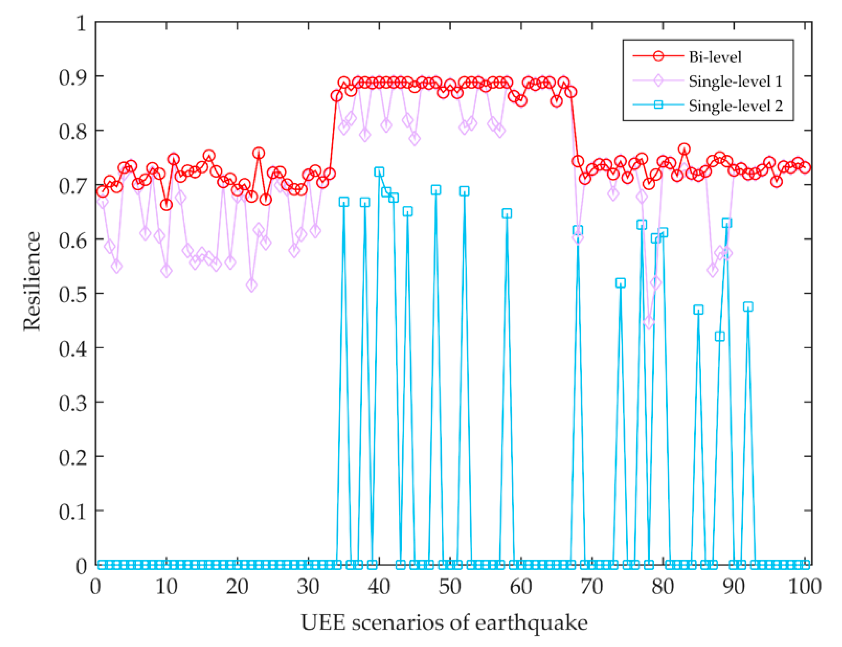
For all UEE scenarios involving an earthquake, the point resilience of the test PHCLTS obtained using the bi-level programming model is the best (
Figure 10). For the results of single-level programming model 2, the point resilience of the test PHCLTS under more than 80% of UEE scenarios is 0. The reason is that the container demands of shippers are ignored in single-level programming model 2. Consequently, the transportation process of containers cannot be completed in the recovered PHCLTS via this model. When studying the resilience problem of PHCLTSs, not only the goals and behaviors of truck carriers should be considered, but also the demands of shippers, who are another transportation PHCLTS user.
To sum up, single-level programming models cannot help the government implement the optimum recovery decisions to restore PHCLTS capacity. Bi-level programming models can support the government to formulate efficient decisions to improve the resilience of a PHCLTS in the face of UEEs.
5.6. Analysis of the Influence of Demand in Hinterland Points
From a long-term perspective, with economic development, daily transportation demands will increase. For the UEE type involving an earthquake, the resilience levels of the test PHCLTS under different demand levels with a recovery budget of 4000 units are shown in
Figure 11.
With the continuous growth of the demand level, the decreasing rate of the resilience level of the test PHCLTS shows an accelerating trend. The increasing demand makes the freight flows in the PHCLTS considerably saturated, i.e., the PHCLTS redundancy, which refers to the remaining capacity that can be provided by the test PHCLTS aside from completing the transportation demand [
14], decreases continuously. Once a UEE scenario occurs, less redundancy capacity can be employed to deal with it. Therefore, the government can adjust the recovery budget and the decisions of recovery activities in time by using the proposed bi-level programming model in accordance with the changes in demand level. When the daily transportation demand level has increased by 30%, the government should raise the budget to 6000 units to achieve a resilience level no less than the resilience level (0.77) under the original demand level (
Figure 12).
6. Managerial Insights and Conclusions
This study focuses on improving the time resilience of PHCLTSs. Managerial insights are obtained from numerical studies as follows:
- (1)
After the occurrence of UEEs, the implementation of appropriate recovery activities can effectively improve the resilience of PHCLTSs and reduce the negative influence caused by UEEs. When insufficient recovery activities are implemented, the resilience of PHCLTSs will be at a low level. Consequently, the total transportation time of containers will increase, and even the transportation demand in the hinterlands cannot be met, leading to negative effects on the economy and society. Appropriate recovery activities are crucial to reduce the negative effects after a UEE occurrence.
- (2)
The randomness of the negative effect on the test PHCLTS is gradually reduced as the budget increases. The resilience of PHCLTSs follows the law of diminishing returns. The government should prepare an appropriate budget in accordance with possible future UEE types.
- (3)
PHCLTS user behaviors will influence the recovery decisions of the government, thereby affecting the resilience of PHCLTSs. Although facing the same UEE situation, the behavior patterns of PHCLTS users are different, and the government’s decision on the recovery activities also differs. The behaviors of PHCLTS users should be considered when studying this issue to improve the resilience of PHCLTSs.
- (4)
From a long-term perspective, with the continuous growth in demand level, the resilience level of a PHCLTS shows a decreasing trend because the redundancy in the PHCLTS decreases. The government should adjust the recovery budget and the decisions on recovery activities in accordance with the changes in demand level to achieve a satisfactory resilience level of the PHCLTS.
- (5)
The government should correctly predict the behaviors of PHCLTS users and their influence on the resilience of PHCLTSs when making decisions about recovery activities after UEEs. Otherwise, the resilience of PHCLTSs will be ineffectively improved, and resources will not be well utilized. The proposed bi-level programming models in this study can support the government in selecting a reasonable budget level and implementing efficient recovery decisions to improve the resilience of PHCLTSs in the face of UEEs.
In this study, a medium- and long-term perspective, which focuses on the time resilience of logistics transportation systems under multiple transportation periods after UEEs, is adopted. A bi-level programming approach is applied to analyze the resilience problem of PHCLTSs. The topological structure of a PHCLTS infrastructure, the goals and behaviors of the PHCLTS planner and users, and their interactions are involved in the bi-level programming model. In consideration of the characteristics of the bi-level programming model, an algorithm combining the PSO algorithm and a traditional optimization algorithm realized using the TOMLAB/CONOPT solver is developed to solve the model.
The proposed bi-level programming models considering the hierarchical relationship and interaction among different participants can support the government in selecting a reasonable budget level and implementing efficient recovery decisions to improve the resilience of PHCLTSs in the face of UEEs. This study analyzes how to improve the resilience of PHCLTSs under UEE situations. It expands the prearranged planning about UEEs and provides a decision-making reference and scientific theoretical support for efficient response to UEEs.
Several implications are available for future research. First, only single mode PHCLTSs were studied, which can be extended to multimodal PHCLTSs. Second, the pre-disaster activities can be studied to obtain a PHCLTS with higher resilience. Third, algorithms for the bi-level programming model can be further developed to improve solving efficiency and validity.


