Abstract
Herein, a finite discrete element method was used to simulate the rockburst phenomenon of elliptical caverns with different axis ratios. Two situations were employed, namely when the disturbance direction is perpendicular and parallel to the ellipse. Based on the peak stress, maximum velocity, stress nephogram, and image fractal characteristics, the influence of axis ratio and direction of the disturbance on rockburst were analyzed. The results show that the samples with different axis ratios experienced the same process of quiet period, slab cracking period, and rockburst. The rockburst pit had V shape, and the failure modes of rockburst primarily included shear cracks, horizontal tension cracks, and vertical tension cracks. With the rise in axis ratio, the peak stress and maximum speed increased. Furthermore, the pressure area on the left and right sides of the sample cavern decreased when the disturbance direction was parallel to the short axis of the ellipse, while it increased for the sample with a disturbance direction perpendicular to the short axis. The fractal dimension value of the crack was gradually amplified with disturbance. The fractal dimension value of the sample whose disturbance direction was perpendicular to the minor axis of the ellipse was lower, and it was more difficult to damage.
1. Introduction
Tunnel is the main part of underground engineering [1,2]. Tunnel construction will face many risks and disasters. Rockburst is a common disaster in underground engineering. Rockbursts have caused great damage to the construction of projects, severely impacting the construction progress and safety of personnel, as shown in Figure 1 [3,4]. Therefore, research on the mechanism of rockburst is of great significance in the construction arena. The current research on the rockburst mechanism has primarily focused on laboratory tests. With the development of science and technology, an increasing number of numerical analysis software sets have been developed. Numerical analysis software sets have the advantages of a low cost and ease of operation, and can provide information that cannot be obtained in experiments; hence, they are widely used in rockburst research. The emergence of related numerical software has greatly promoted the development of rock mechanics and has provided a convenient and effective method for the design and analysis of on-site engineering [5]. Scholars have conducted numerous numerical simulations on the rockburst problem and have obtained valuable results. Common rockburst simulation methods include finite element methods (FEM), finite difference methods (FDM), discontinuous deformation methods (DDA), discrete element methods (DEM), etc.
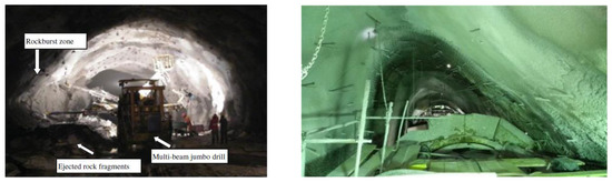
Figure 1.
The pictures of an on-site rockburst [3,4].
In terms of FEM research, Mitri [6] established a numerical analysis model using a finite element method, and analyzed the possibility of rockburst induced by mining using the energy release rate and strain energy storage rate. Bardet [7] used finite element methods to detect the surface instability of bulky solid masses, and provided a numerical technique to analyze rockburst as surface buckling. Wang et al. [8] calculated the strain energy of a coal pillar model before and after failure using ANSYS, and estimated the ejection velocity of the fragments. Zhu et al. [9] employed a Rock Failure Process Analysis System (RFPA) to study the influence of lateral pressure and disturbance on rockbursts with circular caverns. In terms of FDM research, Li et al. [10] compared the overburden structural characteristics and distribution of stresses around roadways and coalfaces in slice mining and top-coal caving mining in thick coal seams via FLAC3D numerical simulation. They analyzed the effects of two mining methods on rockburst prevention. Qi et al. [11] used FLAC to compare the differences between coal bursts, rockbursts, and mine earthquakes. Feng et al. [12] analyzed the roof movement, stress distribution, and elastic strain energy evolution law of the working face by employing different strengths for the backfill-rocks using FLAC3D. They proposed a method to reduce the risk of rockburst by quantitatively adjusting the strength of refilled rocks. In terms of DDA method research, Hatzor et al. [13] used the DDA method to estimate the total kinetic energy released during rockburst and validated the DDA results using monitored seismic energy emissions during an intensive rockburst event while excavating one of the headrace tunnels at Jinping II hydroelectric project in China. Sun et al. [14] employed the combination of DDA and RFPA to simulate the rockburst phenomenon during the excavation of a circular cavern. He et al. [15] used the DDA method to obtain kinetic energy, elastic strain energy, and dissipated energy in the affected zone in a discontinuous rock due to tunneling. In the research of the DEM method, Wu et al. [16] used PDC3D to simulate the unloading rockburst and studied the meso-fracture phenomenon and process under different stress states. Hu et al. [17] employed 3DEC to simulate the rockburst phenomenon induced by a weak continuous disturbance in the tangential direction under the conditions of true triaxial loading and single-sided unloading, and simulated the damage evolution process of rockburst under small cyclic disturbances. He et al. [18,19] used PFC2D to assess the influence of the bedding angle of sandstone and stiffness of the experimental system on the rockburst phenomenon under the conditions of true triaxial loading and single-sided unloading.
The methods used in the above studies are mostly continuous or discontinuous models, both of which have inherent shortcomings. The continuous model cannot simulate the progressive failure process of the rock and cannot simulate large deformation and failure phenomenon. The discontinuous model cannot calculate the rupture inside the block element. Based on the deficiencies of the above research methods, scholars have explored a finite discrete element method (FDEM) [20]. This method can be used to perform decent simulations of an intact rock mass and a discontinuous rock mass. Some scholars have employed the FDEM method to simulate the failure of rocks. Cai [21] conducted FDEM numerical simulations for Brazilian splitting experiments and discussed the impact of the friction coefficient of prefabricated cracks on crack initiation and propagation. Hamdi et al. [22] used an FDEM method to simulate the conventional triaxial and Brazil splitting experiments and compared the failure mode of the sample with the strength criterion in the numerical simulations. Mahabadi et al. [23] employed the Y-Geo program to perform the Brazilian splitting simulation, compared the simulation results with actual phenomena, and obtained good experimental results. Using the Y-Geo program, related scholars have conducted numerous numerical simulations [24,25,26,27], which confirm the effectiveness of this method. As an important tunnel section structure, elliptical section tunnel structures are widely used in practical engineering. However, there is little research into rock burst processes and the mechanisms of elliptical tunnel structures. Therefore, relevant researches are urgently needed to provide a reference for practical engineering. Herein, the Y-Geo program was used to conduct an impact rockburst simulation test of an elliptical cavern with different axis ratios. The development process of rockburst in an elliptical cavern has been summarized, and the influence of the axis ratios on rockburst in an elliptical cavern are compared and analyzed. Moreover, the characteristics of rockbursts under the conditions of disturbance direction perpendicular to and parallel to the minor axis of the ellipse are discussed. This work can provide a reference for the construction of elliptical tunnels.
2. Y-Geo Program Method
Y-geo is a geotechnical analysis program based on an FDEM numerical method. The numerical simulation program was first developed by Munjiza [20], which considering the deformation criteria and failure criteria of geotechnical materials, and combining many detection and judgment criteria. The main criteria included in Y-Geo are quasi-static friction law, Mohr-Coulomb failure criterion, rock shear strength criterion and a dissipative impact model. At the same time, the in-situ stress, material mapping function and the combination of material heterogeneity and transverse isotropy can be considered, which makes Y-Geo suitable for the solution of most engineering failure problems. Y-Geo mainly includes 11 data structure files in the calculation, namely YDC, YDE, YDI, YDN, YDO, YDPE, YDPI, YDPM, YDPN, YDB and YDS, in which each data structure is a part of determining the basic characteristics of the model unit, and different data structures represent the special attributes of the model. In the process of numerical simulation, the parameters in these data structures need to be adjusted to achieve the purpose of numerical simulation of geotechnical problems.
The Y-Geo program method combines the basic principles of a finite element and a discrete element, and can simulate the entire process from continuous to discontinuous. The key to this process is to insert a cohesive element with 4 nodes between adjacent triangular elements. As per the theory of non-linear elastic fracture mechanics, these cohesive units can achieve two modes of failure in the plane state, namely type I fracture and type II fracture. When the tensile displacement of the tip of the cohesive element reaches the yield point 0p from 0, the adjacent triangular elements separate, which results in type I (tensile) fracture. When the relative slip distance of adjacent triangle elements reaches the yield point sp from s, the adjacent triangle elements slip, resulting in type II (shear) fracture; and the shear strength of the cohesive unit follows the Mohr-Coulomb strength criterion [26]. When the cohesive unit of the model cracks and causes local damage, the micro-cracks continue to expand. These cracks finally merge to form a macroscopic through-crack, which leads to a decrease in the model’s load-bearing capacity. The crack formation and fracture modes are presented in Figure 2.
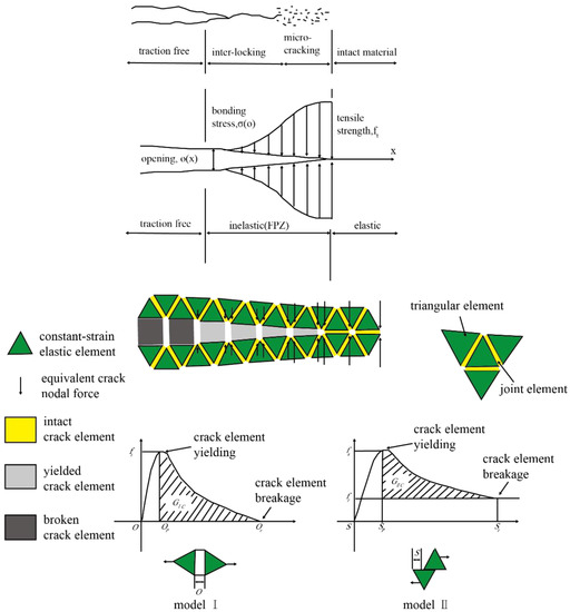
Figure 2.
Basic principle of FDEM numerical simulation. Adapted from Ref. [28].
To make the numerical values closer to the results of laboratory experiments, it was necessary to simulate uniaxial compression experiments and adjust the parameters within a reasonable range. Then, the numerical simulation of impact rockburst of the elliptical cavern was conducted with different axis ratios. The influence of axis ratios on the failure mode of elliptical cavern was analyzed using numerical simulation results.
3. Simulations of Impact Rockburst in Elliptical Cavern
3.1. Determination of Numerical Simulation Parameters
A pre-processing software, Ls-prepost, was used to establish a model with size of 50 × 100 mm, which was used to simulate the uniaxial test. The solid model was divided into freely arranged triangular grids. The size of the triangular element was 1 mm, which can significantly reduce and control the sensitivity of the grid. Then, the built grid was converted into a text file suitable for Y-Geo and the calculation was performed. The uniaxial compression test was simulated and checked via a continuous adjustment of parameters.
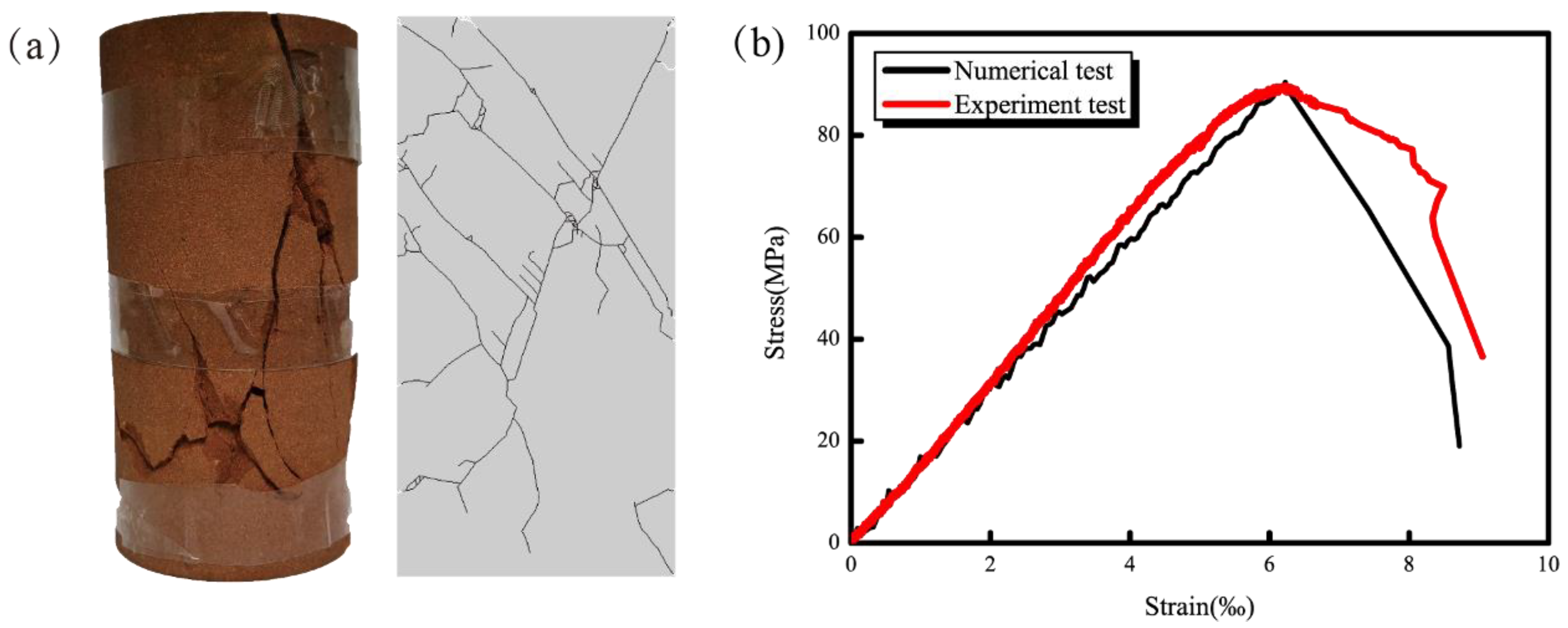
A uniaxial compression test is the main experimental method to measure rock strength. In the numerical simulation test, the lower end of the sample was fixed, and the upper end was loaded at a rate of 0.1 MPa /s until the sample was damaged. Figure 3 shows the numerical simulation of uniaxial compression simulation test failure and stress-strain curve, which has the same characteristics as the laboratory failure. The main performance of the simulated test was shear failure. As per the simulation test, uniaxial compressive strength was 87.59 MPa, which is basically the same as that obtained by laboratory uniaxial compressive strength (87.07 MPa). Furthermore, the strain value in simulation was close to that in the laboratory test. Hence, it can be concluded that the parameters selected in these simulations can represent rock properties. The specific mechanical parameters are listed in Table 1. Density, elastic modulus, and Poisson’s ratio represent the basic properties of the rock mass, and viscous damping, tangential penalty factor, normal penalty factor, and fracture penalty factor are expressed in the stiffness characteristics of the rock mass, the tensile strength, cohesion, internal friction angle and fracture energy represent the strength characteristics of the rock mass.

Figure 3.
Uniaxial compression simulation experiment (a) comparison between simulation and laboratory experiment; (b) stress-strain curve.

Table 1.
Mechanical parameters of numerical model of sandstone.
3.2. Model Establishment
Figure 4 displays the numerical simulation model of this article. σh is the horizontal confining pressure, σv is the gravity stress, and σD is the disturbance load. The simulation selects a stress level of 500 m, where σh is 10.2 MPa, σv is 13.6 MPa, and σD is the slope disturbance loading method. The long axis of the ellipse is a and the short axis is b. According to the positional relationship between the disturbance direction and the short axis of the ellipse, two test types were set, namely, the disturbance direction is parallel and perpendicular to the short axis of the ellipse. The size of the sample was 110 × 110 mm with an oval cavity in the middle.
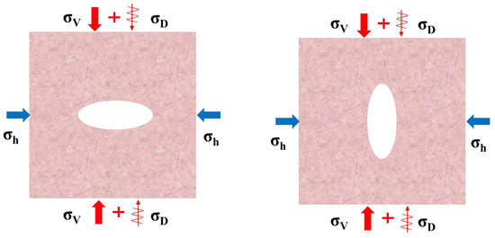
Figure 4.
Schematic diagram of numerical simulation model.
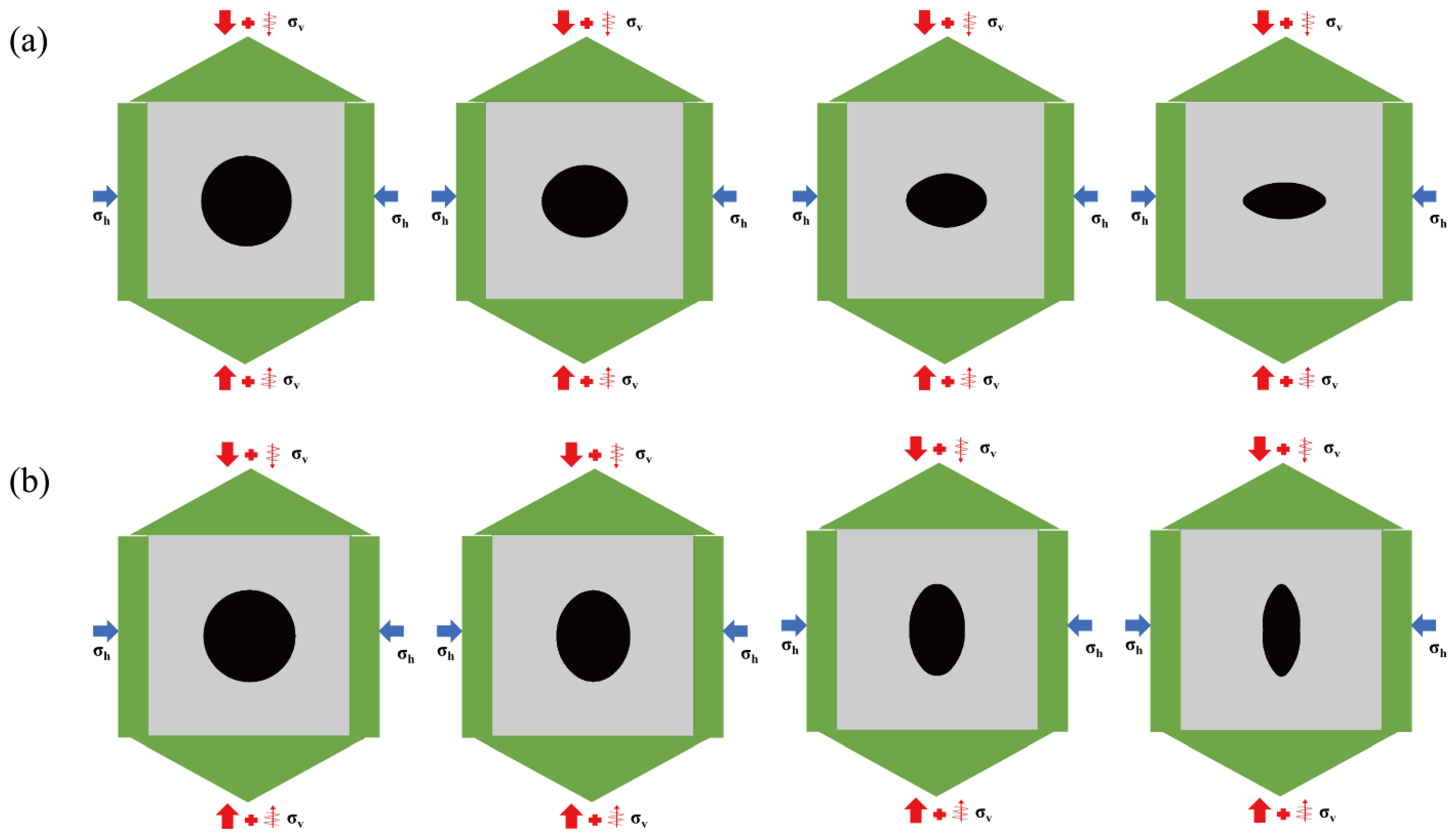
The primary objective of this work was to simulate rockbursts under different long–short axis ratios. The fixed long axis was 50 mm, while the short axis directions were 50 mm, 40 mm, 30 mm, and 20 mm. Hence, the long and short axis ratios were 1, 1.25, 1.67, and 2.5. Considering the two situations where the disturbance direction was parallel to and perpendicular to the short axis of the ellipse, the numerical model diagrams shown in Figure 4 were established. Figure 5a presents a numerical model with the disturbance direction parallel to the short axis, and Figure 5b displays a numerical model with the disturbance direction perpendicular to the short axis. Notably, the shape of the sample with a short axis of 50 mm was circular, and the circle is a special kind of ellipse. In the simulation test, the lower part is the fixed end, and the load is applied on the left, right and upper sides. According to the principle of force balance, when a load is applied above the sample, the same reaction force is received below the sample. Table 2 lists the specific model size and number, named after the relationship between disturbance direction and short axis and length. H-30 and V-30 are used as examples, where H represents the disturbance direction, which was parallel to the short axis, V represents that the disturbance direction was perpendicular to the short axis, and 30 represents the length of the short axis of the ellipse. H-50 and V-50 refer to the same sample.
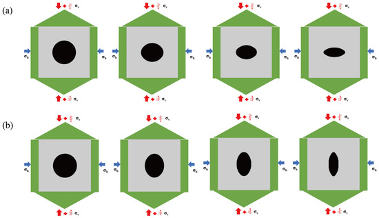
Figure 5.
Numerical simulation model of different axis ratios: (a) direction of disturbance is parallel to the short axis; and (b) disturbance direction is perpendicular to short axis.
Table 2.
Numerical simulation model sizes with different axial ratios.
3.3. Simulation Results
3.3.1. Loading Stress Path
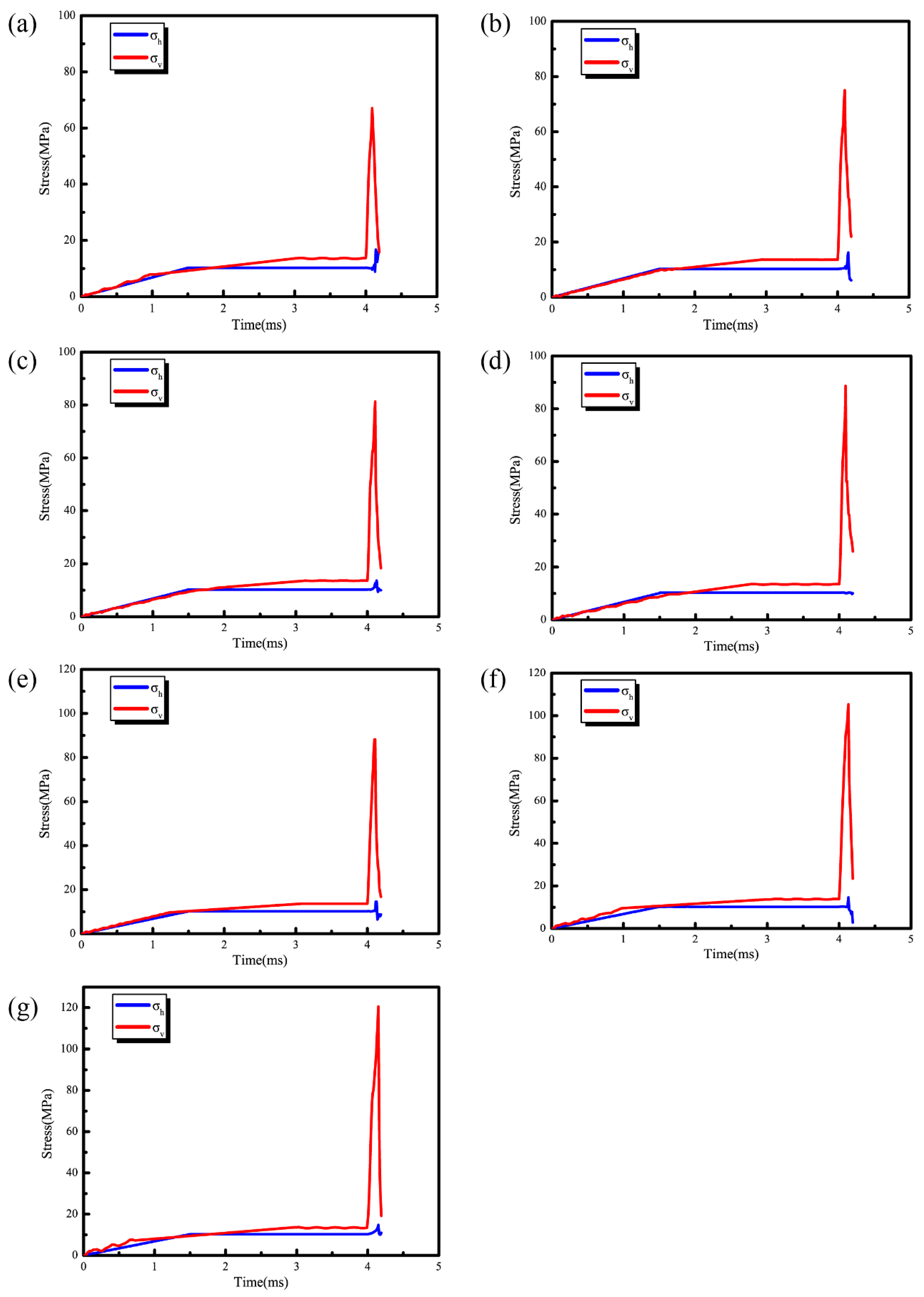
Figure 6 shows the loading stress path with different axis ratios. At 1.5 ms, the horizontal direction stress first reached the preset stress level, and the horizontal stress σh was 10.2 MPa. Then, the load was slowly applied in the vertical direction. At 3.0 ms, the vertical direction stress reached the preset stress level, and its value σv was 13.6 MPa. At this time, the samples were already at the initial stress level of 500 m. Under this stress level, the load was maintained for 1 ms, and finally, a large impact disturbance was quickly applied for the duration of 0.2 ms.
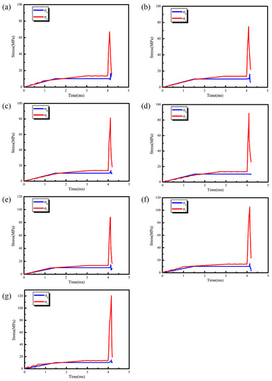
Figure 6.
Numerical simulation loading path of specimens with different axial ratios (a) H-50 (V-50), (b) H-40, (c) H-30, (d) H-20, (e) V-40, (f) V-30, and (g) V-20.
As per the figure, the simulation tests with different axis ratios exhibited the same stress path during the loading process. After the disturbance was applied, the vertical stress increased rapidly and reached the peak level. Subsequently, the sample suffered macroscopic damage, its bearing capacity decreased, and the vertical stress value dropped rapidly. Moreover, as per the Poisson’s ratio of the material, the horizontal stress simultaneously fluctuated to varying degrees during the rises in vertical stress.
3.3.2. Simulation Process
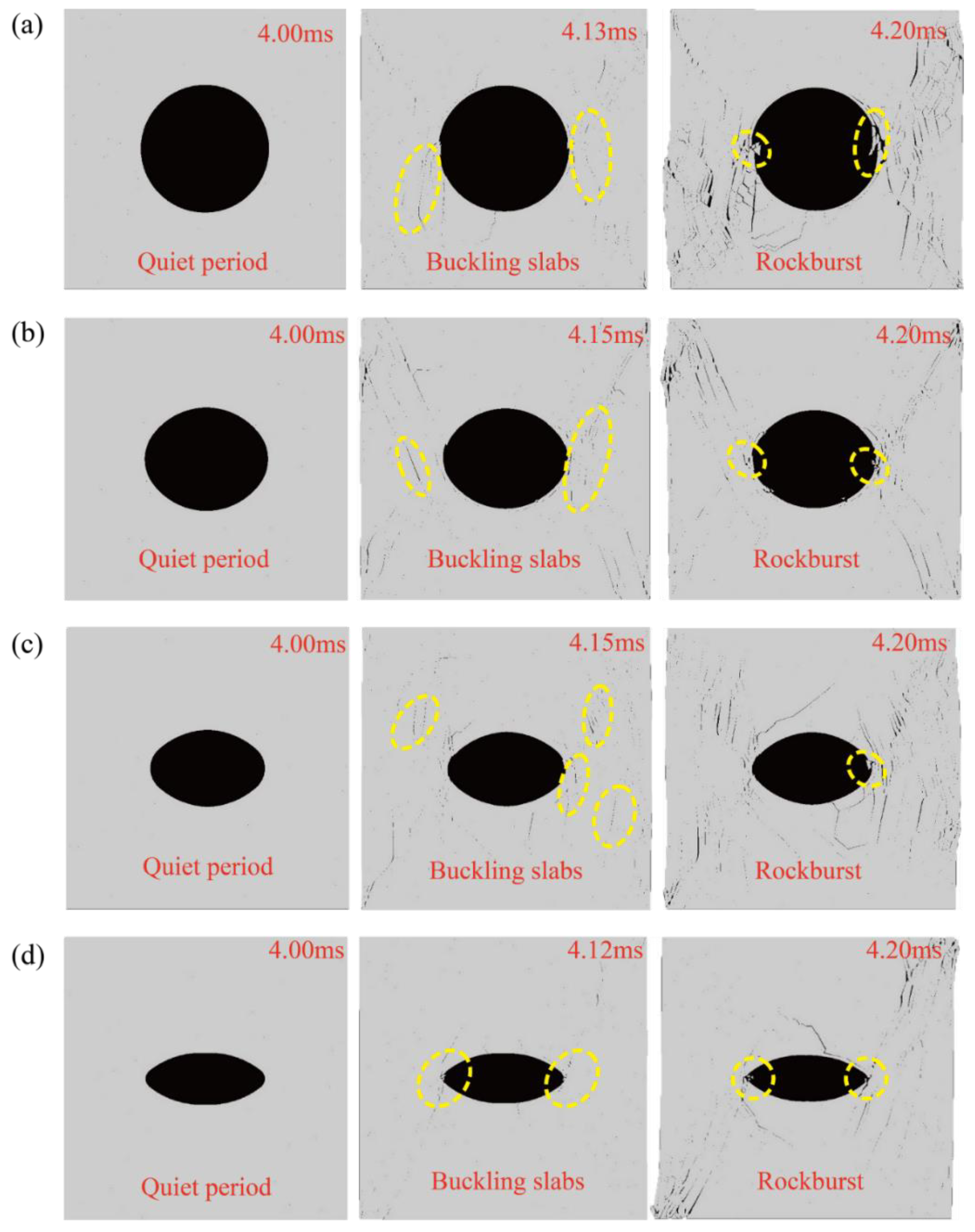
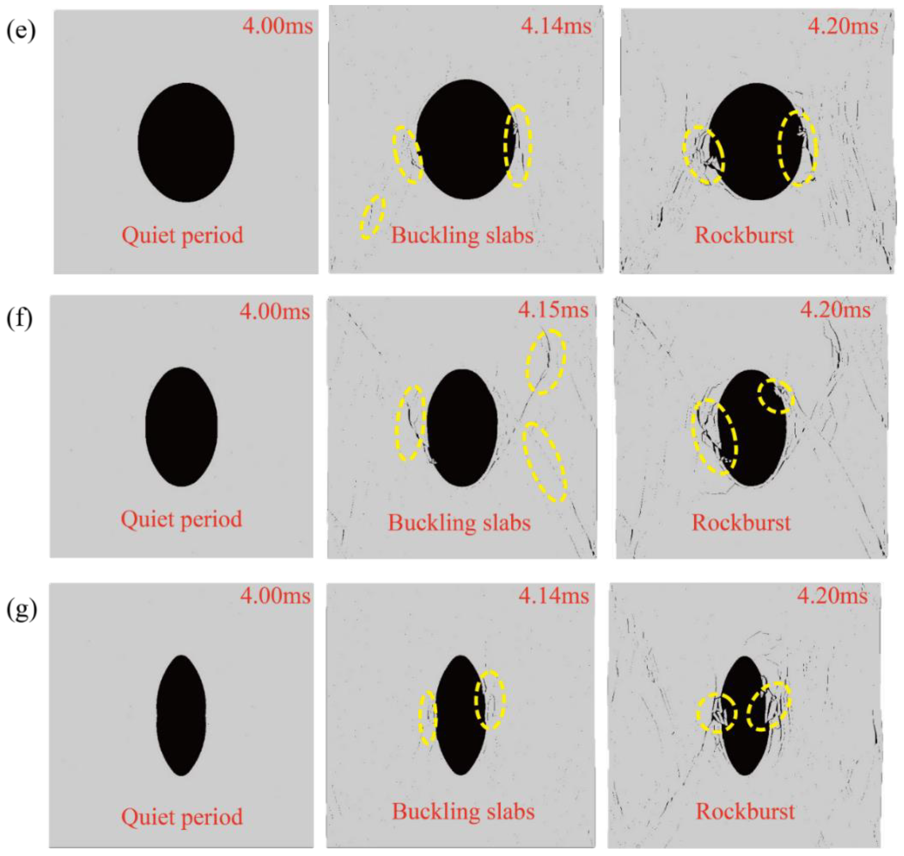
Figure 7 shows the typical damage phenomena in simulations with different axis ratios. The simulation tests with different axis ratios underwent the same process during loading, primarily including the quiet period, slab cracking period, and the rockburst period. Using the H-50 sample for illustration, when the sample was loaded to the initial stress level, the stress level was relatively low, the sample was in a relatively stable state, and no prominent damage was observed. At this time, the sample was in a quiet period. In this process, the sample was compressed and deformed, and a part of the energy was stored. However, the energy did not exceed the energy required for the destruction of the sample. With the application of the disturbance load, the load on the sample exceeded the load required for its failure and prominent cracks were produced on the left and right sides of the sample. As the load was enhanced, the length and number of cracks gradually increased, but the cavern did not produce large deformation and failure, and the sample was in a slab cracking period. With the continuous application of the disturbance load, a fragment on the left side of the cavern was ejected at a certain speed and a large piece of fragment was separated from the right side of the cave. Simultaneously, cracks became more prominent on the left and right sides, away from the cavern. The sample at this time was already in a severely damaged stage, i.e., it had entered the rockburst period.
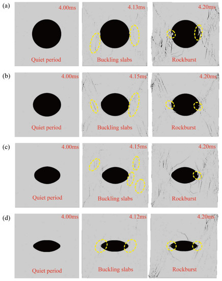
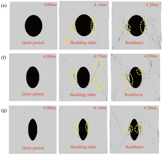
Figure 7.
Typical phenomena in numerical simulation experiments with different axial ratios: (a) H-50 (V-50); (b) H-40; (c) H-30; (d) H-20; (e) V-40; (f) V-30; and (g) V-20.
4. Results and Discussion
4.1. Failure Mode
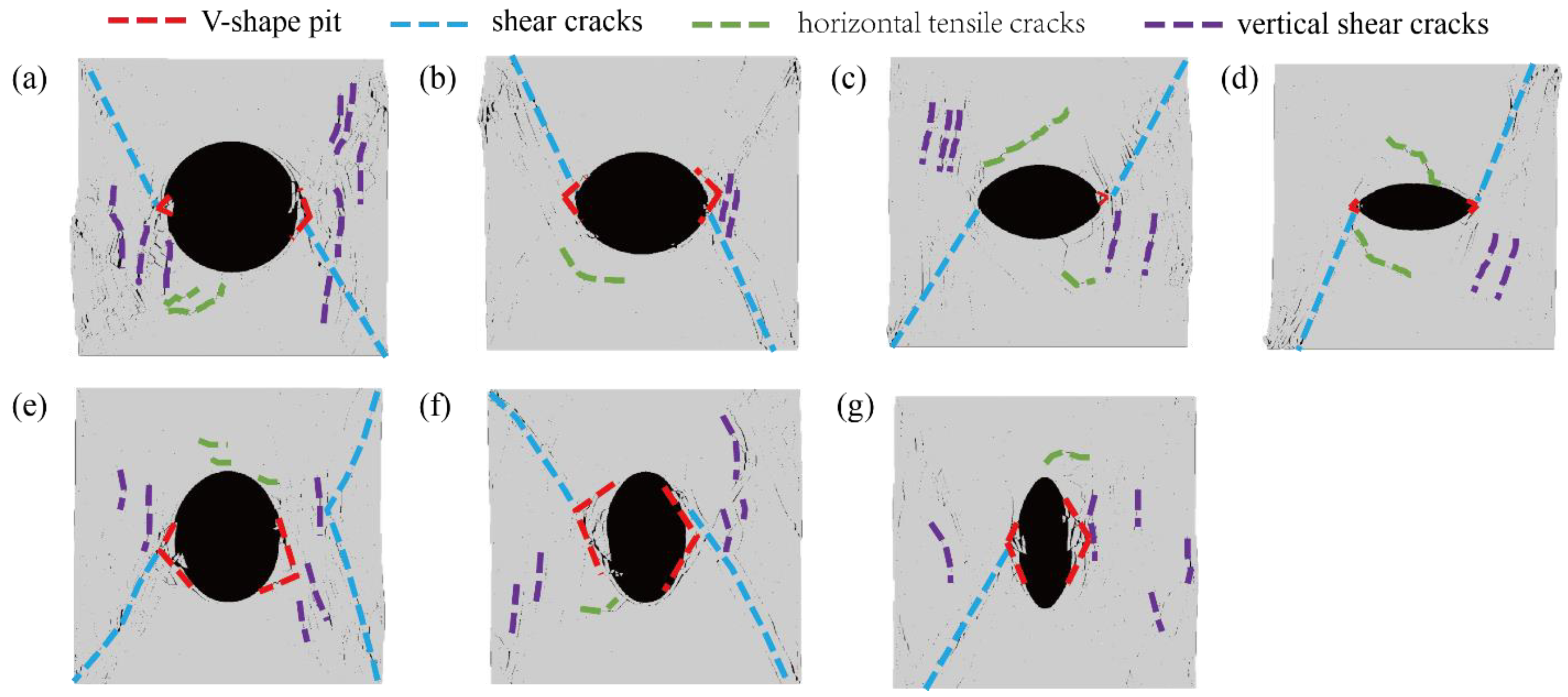
Figure 8 displays the numerical simulations after the rockburst. With regards to the shape of the rockburst pit, all the pits of the samples presented the V shape. Notably, as the fragments were not completely ejected in the simulations, the shape cannot be called V-shaped. However, the development trend of the crack can be estimated to be V-shaped as per the shape of the crack. Due to the disturbing load, the sample produced an oblique shear crack, which penetrated from the pit damage position to the upper and lower surfaces of the sample, forming an oblique shear crack penetrating the cavity. A certain angle forms through shear failure. While oblique shear cracks were generated, horizontal and vertical tensile cracks appeared around the cave wall, and these two types of cracks were connected with oblique shear cracks. The damage of the sample is mainly shear failure. There are tensile stresses above and below the cavern, and so horizontal tensile cracks appear. Due to the excavation of the cavern, there is unloading on the left and right sides of the cavern. Due to the vertical pressure and unloading, vertical tension cracks appear on the left and right sides of the cavern. The above three types of cracks appeared in the simulation experiments. It can be seen that the larger the axis ratios, the larger the shape of V-shaped pits.

Figure 8.
The failure modes with different axis ratios (a) H-50 (V-50), (b) H-40, (c) H-30, (d) H-20, (e) V-40, (f) V-30, and (g) V-20.
4.2. Maximum Stress during Experiment
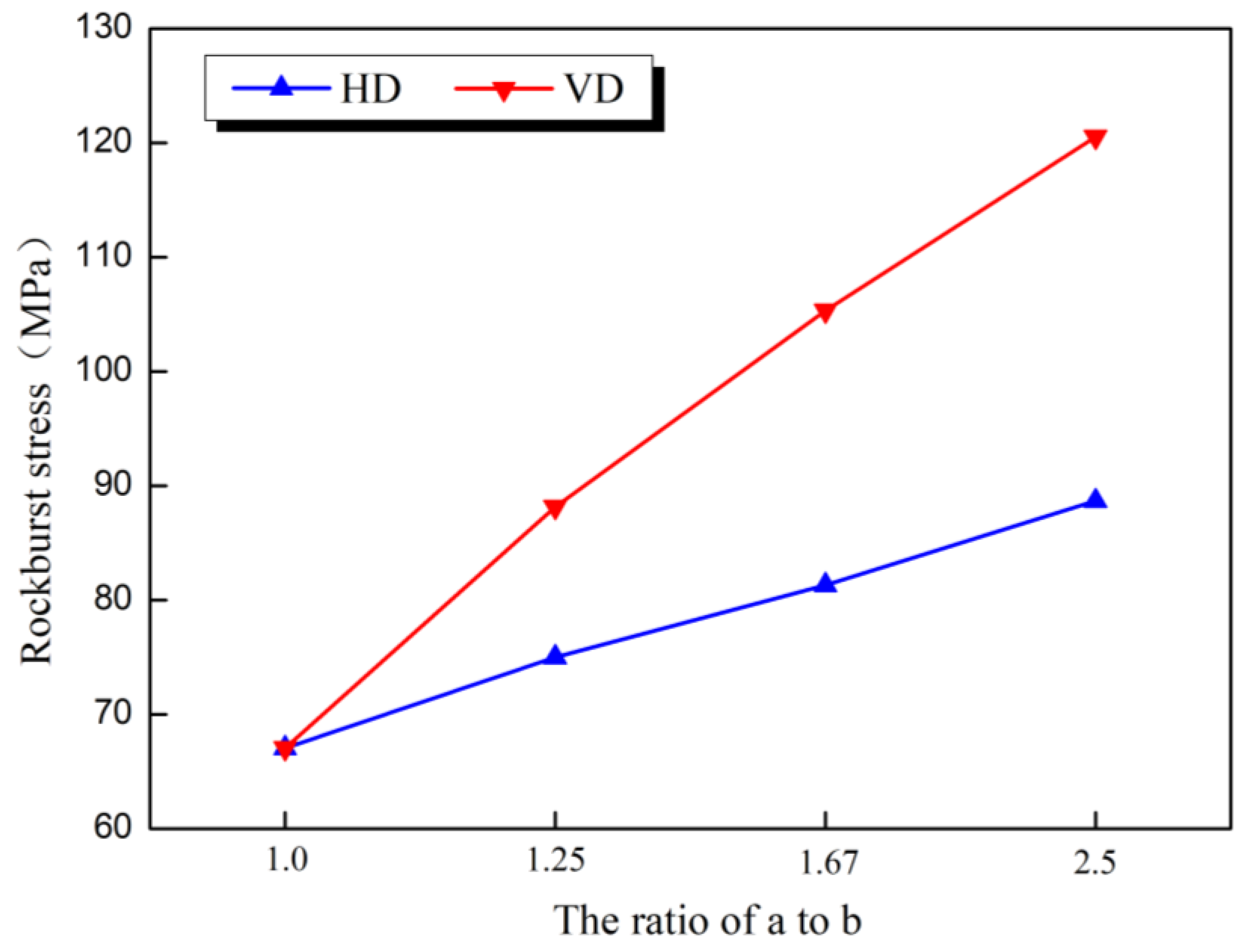
Figure 9 shows the relationship between the peak stress and axis ratios as per Section 3. With the increase in axis ratios, the peak stress level in the numerical simulation displayed an approximately linear increase, i.e., the larger the axis ratio, the higher the peak stress. Under the same axis ratio conditions, the peak strength value of the VD sample was higher, indicating that the load level was higher. These results show that the sample with the disturbance direction perpendicular to the short axis of the ellipse can clearly increase the bearing capacity of the cavern structure and slow the damage of the rockburst.
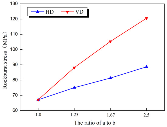
Figure 9.
Relationship between rockburst stress and axial ratios.
4.3. Maximum Speed of Experimental Process
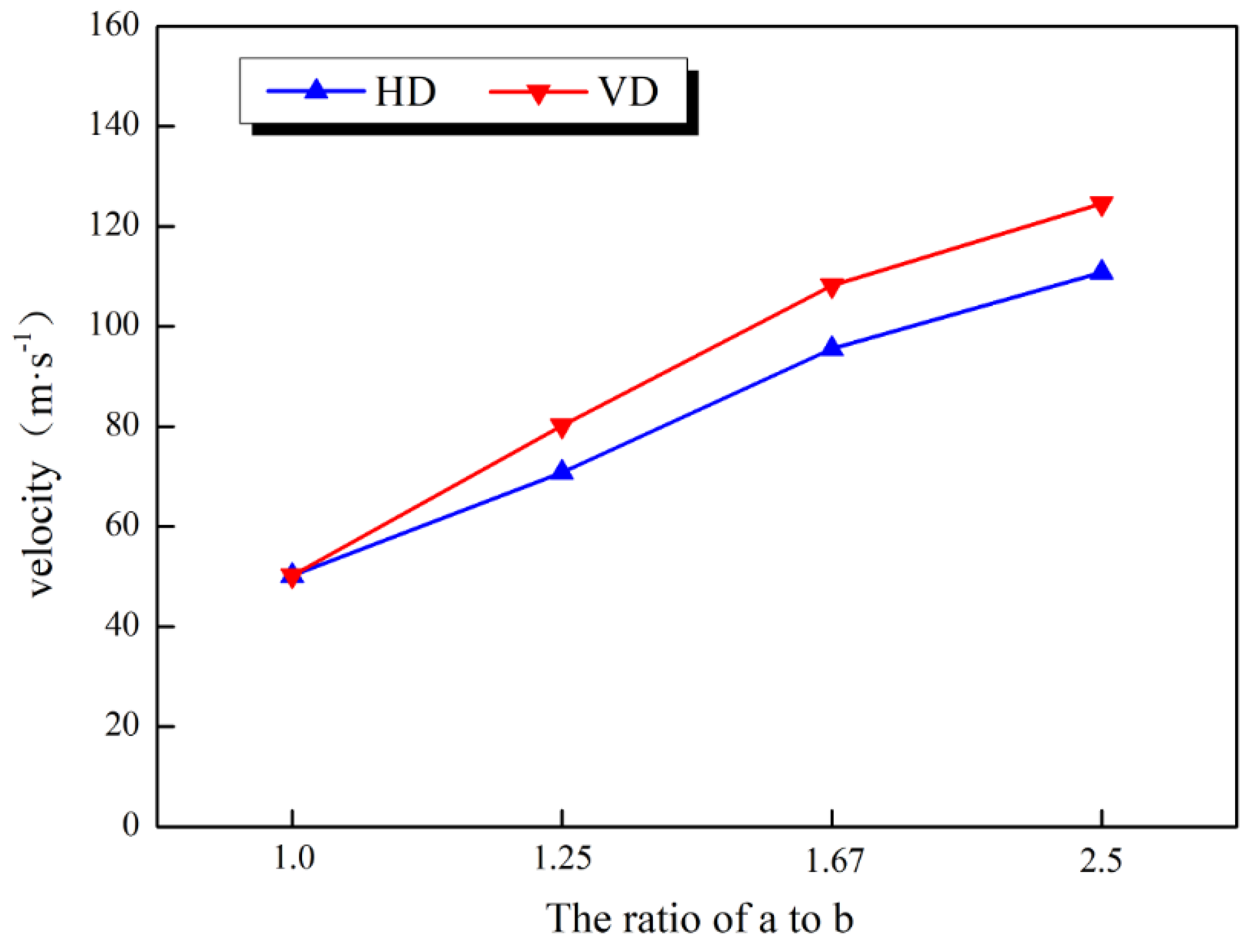
According to the results of numerical simulation, maximum ejection velocity of the simulated samples with different axis ratios were extracted. Figure 10 shows the relationship between maximum ejection velocity of the numerical simulations and axis ratios. With the rise in axis ratio, the maximum ejection speed was also increased. Under the same axis ratio, maximum ejection velocity of the VD sample was higher than the HD sample. As per Section 4.2, the stress on the sample was greater when the disturbance direction was perpendicular to the short axis of the ellipse. Therefore, the larger the accumulated energy, the greater the energy released during the disturbance process, and the higher the velocity generated.
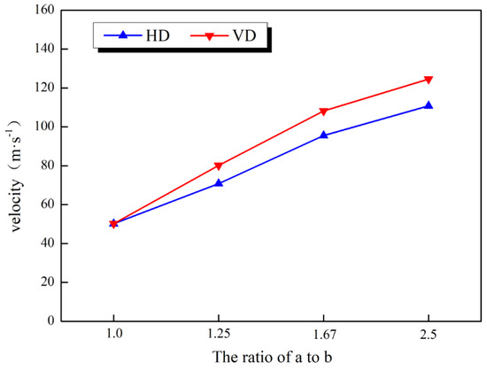
Figure 10.
Relationship between maximum average ejection velocity and axial ratios.
4.4. Stress Nephogram
Figure 11 shows the stress nephogram of samples with different axis ratios. The selected moment was 0.8 times that of the peak stress. All the samples displayed the same characteristics on the stress nephogram. There were areas of compressive stress on the left and right sides of the cavern, while the tensile stress acted on the upper and lower sides of the cavern. The compressive stress value was significantly higher than the tensile stress. Owing to the compressive stress, the damage range of the elliptical cavern was on the left and right sides of the cavern. For HD samples, with the rise in axis ratios, the compressive stress area on the left and right sides of the cavern decreased, while the tensile stress area of the upper and lower cavern increased. For VD specimens, the change in trend was opposite. As the axis ratios increased, the area of compressive stress amplified, while the area of tensile stress was reduced.
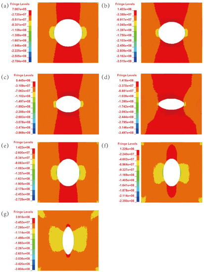
Figure 11.
Stress nephogram of samples with different axial ratios (a) H-50 (V-50), (b) H-40, (c) H-30, (d) H-20, (e) V-40, (f) V-30, and (g) V-20.
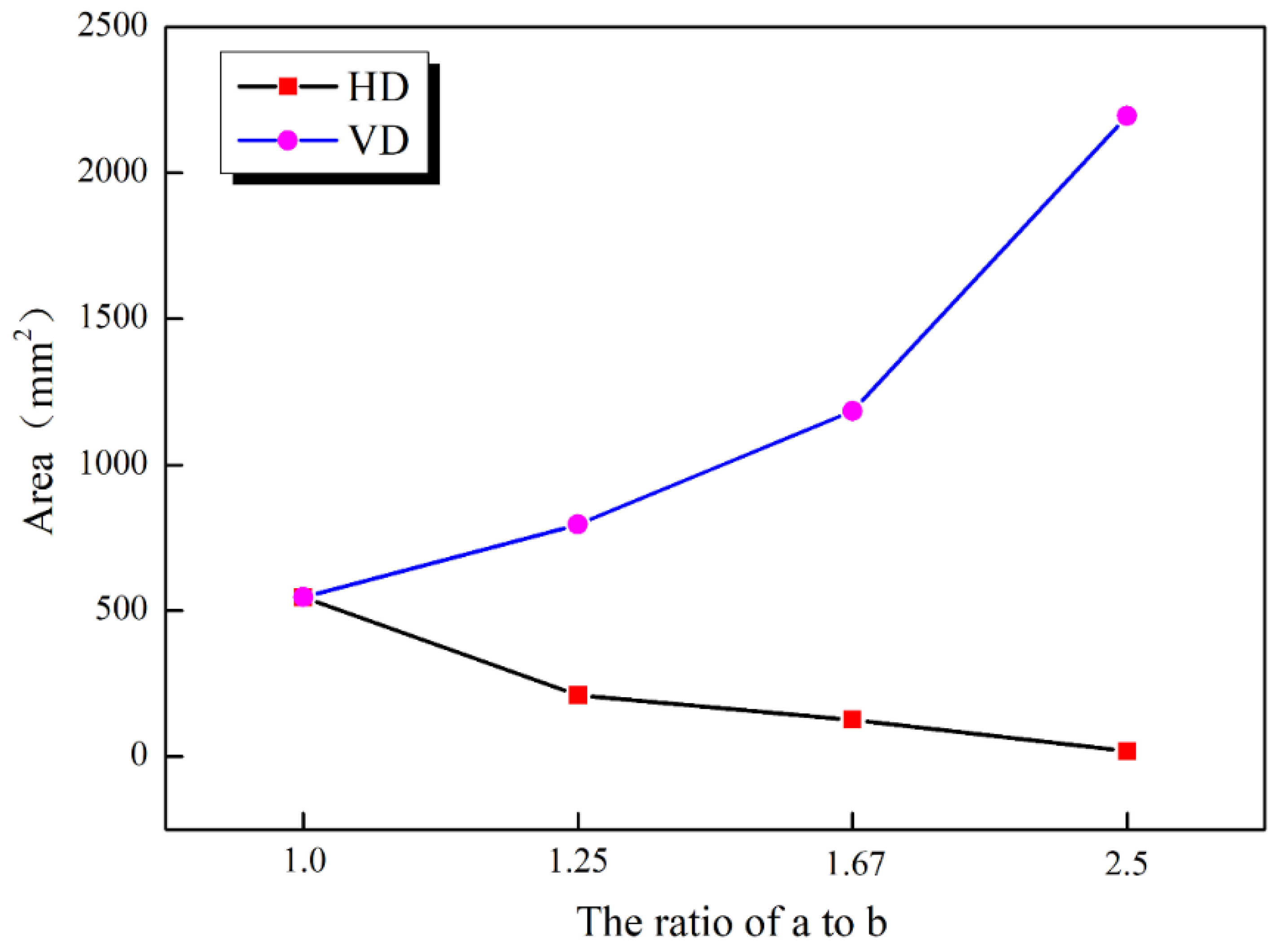
According to the stress nephogram, the area of the compression zone was extracted using an image processing software, and the relationship curve between the compression zone area and the axis ratios was drawn (see Figure 12). With the rise in ratio of the length to short axis, the compression area of the HD sample decreased, while the compression area of the VD sample increased.
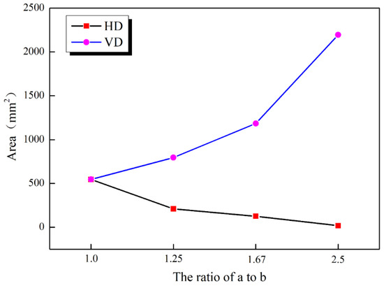
Figure 12.
Relationship between compression area and axial ratios.
4.5. Fractal Characteristics of Crack Images
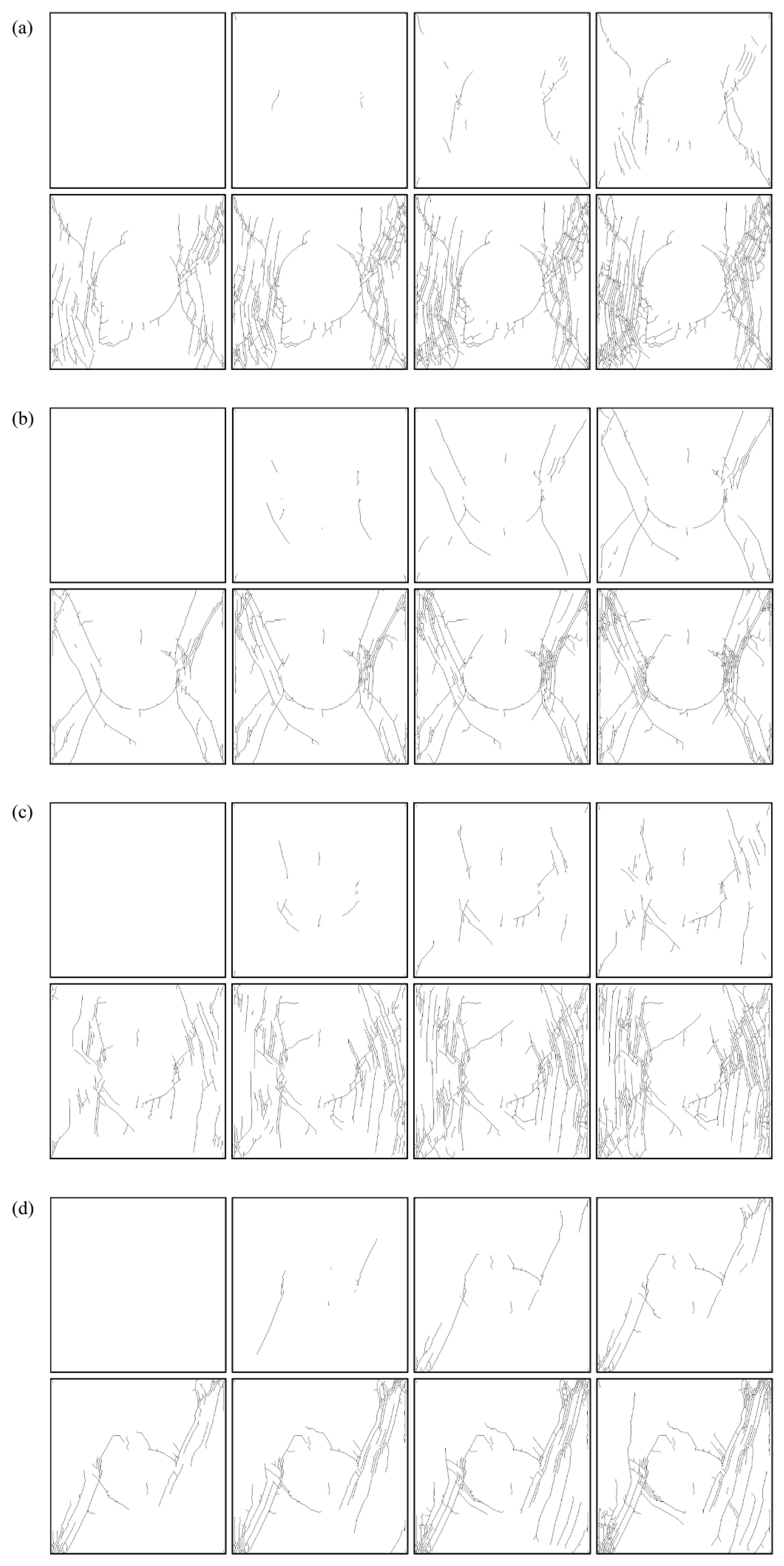
In the process of numerical simulations, with the vertical disturbance load, the generation and propagation of cracks occurred. The presence of cracks signifies that the sample has been damaged, and the number of cracks reflect the damage degree of the sample. To observe the development process of cracks more clearly, the images of the sample were processed into a binary image containing only black and white using image processing software, and the cracks were represented in black. Figure 13 shows the crack development process of the numerical simulation specimens with different axis ratios. With the disturbance load, the cracks increased. The crack evolution diagram reflects the entire failure process of the sample, and also shows the failure location.
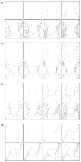
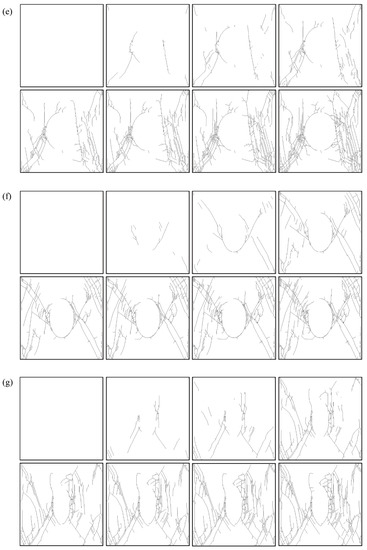
Figure 13.
Crack evolution of samples with different axial ratios (a) H-50 (V-50), (b) H-40, (c) H-30, (d) H-20, (e) V-40, (f) V-30, and (g) V-20.
Several studies have proved that the crack structure in the rock exhibits a certain degree of self-similarity [29]. To compare and analyze the crack differences of samples with different axis ratios, the fractal theory has been employed. Herein, a covering method was used to study the fractal parameter values of cracks. The calculation formula of fractal dimension is
where δk is the side length of the square grid, Nδk (F) is the number of square grids covered by cracks, and D represents the fractal dimension. The greater the fractal dimension, the larger the degree of damage.
Equation (1) was used to calculate the value of fractal dimension of the image crack in the whole process. The relationship between the fractal dimension and loading time was drawn as per the obtained results (see Figure 14). There were only incremental changes in the fractal dimension of cracks in all the samples. After 4.09 ms, there was a change in the value of the fractal dimension, indicating that there was a crack at this moment. With the disturbance load, the value of the fractal dimension gradually increased from 0 to maximum, and the distribution range of the fractal dimension of all the samples was 0–1.6.
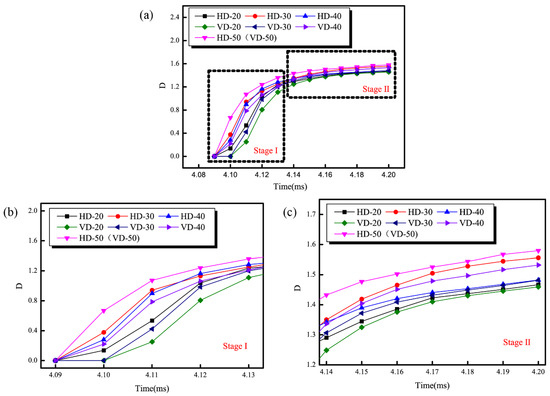
Figure 14.
Change of fractal dimension (a) relationship between fractal value of different axis ratios with time (b) stage I (c) Stage II.
According to the characteristics of the curve, the curve can be divided into two stages. Stage I is the sudden stage. In this stage, the value of the fractal dimension increased rapidly, and the range of variation was 0–1.2, suggesting that the crack grew rapidly at this stage. Due to the strong disturbance load, stage I is the process of the disturbance force increasing to the peak stage. The samples were destroyed rapidly, cracks occurred rapidly, and a sudden change occurred in the value of the fractal dimension. Stage II is a slowly changing stage, wherein the fractal dimension increased slowly, and the range of change was 1.2–1.6. This is because the disturbance stress was reduced at this stage, the stress value decreased, and the number of cracks produced lowered, which led to a decline in the rate of change of fractal dimension.
Figure 14b,c presents the enlarged view of stage I and stage II. At the same moment, the sample of HD-50 (VD-50) was at the top, and the order from top to bottom was HD-30, HD-40, VD-40, VD-30, HD-20, and VD-20. As the axis ratio increased, the value of the fractal dimension decreased. A small value of fractal dimension indicates a low degree of damage. These results demonstrate that during the disturbance process, the greater the axis ratio of the cavern, the more difficult it was to produce rockbursts. Compared with the circular caverns, it was more difficult for rockbursts in the elliptical caverns. Under the same conditions, the fractal dimension of HD samples was higher than that of VD samples. The samples whose disturbance direction was a short axis of the ellipse were more difficult to damage. As per the analysis of fractal characteristics of the crack image, for a fixed axis ratio, the cavity structure was safest when the disturbance direction was perpendicular to the short axis of the ellipse and the damage was lowest. This work can provide a reference for an engineering design.
5. Conclusions
Herein, the impact rockburst tests of an elliptical cavern was simulated for different axis ratios using a finite discrete element method. The main conclusions are as follows:
- The numerical simulation process of impact rockburst with different axis ratios displayed a quiet period, a slab-cracking period, and a rockburst period. The failure modes of the samples primarily included V-shaped blasting pits, diagonal shear cracks, horizontal tension cracks, and vertical tension cracks, which were the same as laboratory failure modes.
- With the increase in an axis ratio, maximum ejection velocity and vertical maximum stress demonstrated an increasing trend. These values were higher for the samples whose disturbance direction was perpendicular to the short axis of the ellipse than for the samples whose disturbance direction was parallel to the short axis of the ellipse.
- Numerical simulation tests confirm that during the loading process, the left and right sides of the elliptical cavity were under a compressive stress, while the upper and lower sides of the cavity experienced tensile stress. The compressive stress value was significantly larger than the tensile stress. With the increase in axis ratio, the pressure area of the samples whose disturbance direction was parallel to the short axis of the ellipse decreased, while the pressure area of the sample whose disturbance direction was perpendicular to the short axis of the ellipse increased and the pressure area was larger.
- With the loading of disturbance, the value of the fractal dimension gradually increased, and its changed process could be divided into two stages: a sudden change and a slow change. The changing trends of the samples with different axis ratios were the same in two stages. Using the fractal dimension value, it can be confirmed that the larger the axis ratio is, the more difficult it is to damage. The samples with a disturbance direction perpendicular to the short axis of the ellipse were most difficult to damage.
Author Contributions
Conceptualization, methodology, supervision, software and funding acquisition, Y.W. and X.L.; validation, formal analysis, data curation, writing—original draft preparation, writing—review and editing, visualization, J.L. and J.X. All authors have read and agreed to the published version of the manuscript.
Funding
This study was supported by the Fundamental Science Foundation of Institute of Geomechanics (DZLXJK202009), China Geological Survey Project (DD20190319) and National Natural Science Foundation of China (42007280).
Institutional Review Board Statement
Not applicable.
Informed Consent Statement
Not applicable.
Data Availability Statement
The source of relevant data acquisition has been described in the text.
Conflicts of Interest
The authors declare no conflict of interest.
References
- Wu, K.; Shao, Z.; Qin, S.; Zhao, N.; Chu, Z. An Improved Nonlinear Creep Model for Rock Applied to Tunnel Displacement Prediction. Int. J. Appl. Mech. 2021, 13, 2150094. [Google Scholar] [CrossRef]
- Wu, K.; Shao, Z.; Sharifzadeh, M.; Chu, Z.; Qin, S. Analytical Approach to Estimating the Influence of Shotcrete Hardening Property on Tunnel Response. J. Eng. Mech. 2022, 148, 04021127. [Google Scholar] [CrossRef]
- Zhang, C.; Feng, X.-T.; Zhou, H.; Qiu, S.; Wu, W. Case Histories of Four Extremely Intense Rockbursts in Deep Tunnels. Rock Mech. Rock Eng. 2012, 45, 275–288. [Google Scholar] [CrossRef]
- Jing, L. A review of techniques, advances and outstanding issues in numerical modelling for rock mechanics and rock engineering. Int. J. Rock Mech. Min. Sci. 2003, 40, 283–353. [Google Scholar] [CrossRef]
- Rehman, H.; Naji, A.; Nam, K.; Ahmad, S.; Muhammad, K.; Yoo, H.-K. Impact of Construction Method and Ground Composition on Headrace Tunnel Stability in the Neelum–Jhelum Hydroelectric Project: A Case Study Review from Pakistan. Appl. Sci. 2021, 11, 1655. [Google Scholar] [CrossRef]
- Mitri, H. Fe modelling of mining-induced energy release and storage rates. J. S. Afr. Inst. Min. Metall. 1999, 99, 103–110. [Google Scholar]
- Bardet, J. Finite element analysis of rockburst as surface instability. Comput. Geotech. 1989, 8, 177–193. [Google Scholar] [CrossRef]
- Liu, G.; Karakus, M.; Mu, Z. Propagation and attenuation characteristics of rockburst-induced shock waves in coal-rock medium. Arab. J. Geosci. 2019, 12, 113. [Google Scholar] [CrossRef]
- Wang, Z.; Li, L. Study of Energy Release in Failure of Coal and Rock Near Fault on ANSYS. Geotech. Geol. Eng. 2019, 37, 2577–2589. [Google Scholar] [CrossRef]
- Zhu, W.; Liu, J.; Tang, C.; Zhao, X.; Brady, B. Simulation of progressive fracturing processes around underground excavations under biaxial compression. Tunn. Undergr. Space Technol. 2005, 20, 231–247. [Google Scholar] [CrossRef]
- Li, Z.-L.; He, X.-Q.; Dou, L.-M.; Song, D.-Z.; Wang, G.-F. Numerical investigation of load shedding and rockburst reduction effects of top-coal caving mining in thick coal seams. Int. J. Rock Mech. Min. Sci. 2018, 110, 266–278. [Google Scholar] [CrossRef]
- Qi, Q.; Chen, S.; Wang, H.; Mao, D.; Wang, Y. Study on the relations among coal bump, rockburst and mining tremor with numerical simulation. Chin. J. Rock Mech. Eng. 2003, 22, 1852–1858. (In Chinese) [Google Scholar]
- Feng, X.; Zhang, Q.; Ali, M. 3D modelling of the strength effect of backfill-rocks on controlling rockburst risk: A case study. Arab. J. Geosci. 2020, 13, 1–16. [Google Scholar] [CrossRef]
- Hatzor, Y.; He, B.-G.; Feng, X.-T. Scaling rockburst hazard using the DDA and GSI methods. Tunn. Undergr. Space Technol. 2017, 70, 343–362. [Google Scholar] [CrossRef]
- Sun, J.-S.; Zhu, Q.-H.; Lu, W.-B. Numerical Simulation of Rock Burst in Circular Tunnels Under Unloading Conditions. J. China Univ. Min. Technol. 2007, 17, 552–556. [Google Scholar] [CrossRef]
- Wu, S.; Zhou, Y.; Gao, B. Study of unloading tests of rock burst and PFC3D numerical simulation. Chin. J. Rock Mech. Eng. 2010, 29, 4082–4088. (In Chinese) [Google Scholar]
- Hu, L.; Ma, K.; Liang, X.; Tang, C.; Wang, Z.; Yan, L. Experimental and numerical study on rockburst triggered by tangential weak cyclic dynamic disturbance under true triaxial conditions. Tunn. Undergr. Space Technol. 2018, 81, 602–618. [Google Scholar] [CrossRef]
- He, M.; Ren, F.; Cheng, C. Mechanism of Strain Burst by Laboratory and Numerical Analysis. Shock. Vib. 2018, 2018, 1–15. [Google Scholar] [CrossRef] [Green Version]
- He, M.; Ren, F.; Cheng, C. Experimental and numerical analyses on the effect of stiffness on bedded sandstone strain burst with varying dip angle. Bull. Int. Assoc. Eng. Geol. 2019, 78, 3593–3610. [Google Scholar] [CrossRef]
- Munjiza, A.; Bangash, T.; John, N.W.M. The combined finite-discrete element method for structural failure and collapse. Eng. Fract. Mech. 2004, 71, 469–483. [Google Scholar] [CrossRef]
- Cai, M. Fracture Initiation and Propagation in a Brazilian Disc with a Plane Interface: A Numerical Study. Rock Mech. Rock Eng. 2013, 46, 289–302. [Google Scholar] [CrossRef]
- Hamdi, P.; Stead, D.; Elmo, D. Damage characterization during laboratory strength testing: A 3D-finite-discrete element approach. Comput. Geotech. 2014, 60, 33–46. [Google Scholar] [CrossRef]
- Mahabadi, O.; Lisjak, A.; Munjiza, A.; Grasselli, G. Y-Geo: New Combined Finite-Discrete Element Numerical Code for Geomechanical Applications. Int. J. Géoméch. 2012, 12, 676–688. [Google Scholar] [CrossRef]
- Elmo, D.; Stead, D.; Eberhardt, E.; Vyazmensky, A. Applications of Finite/Discrete Element Modeling to Rock Engineering Problems. Int. J. Géoméch. 2013, 13, 565–580. [Google Scholar] [CrossRef] [Green Version]
- Lisjak, A.; Liu, Q.; Zhao, Q.; Mahabadi, O.; Grasselli, G. Numerical simulation of acoustic emission in brittle rocks by two-dimensional finite-discrete element analysis. Geophys. J. Int. 2013, 195, 423–443. [Google Scholar] [CrossRef] [Green Version]
- Lisjak, A.; Garitte, B.; Grasselli, G.; Müller, H.J.; Garitte, B. The excavation of a circular tunnel in a bedded argillaceous rock (opalinus clay): Short-term rock mass response and fdem numerical analysis. Tunn. Undergr. Space Technol. 2015, 45, 227–248. [Google Scholar] [CrossRef] [Green Version]
- Mahabadi, O.K. Investigating the Influence of Microscale Heterogeneity and Microstructure on the Failure and Mechanical Behaviour of Geomaterials; University of Toronto: Toronto, ON, Canada, 2012. [Google Scholar]
- Mahabadi, O.; Kaifosh, P.; Marschall, P.; Vietor, T. Three-dimensional FDEM numerical simulation of failure processes observed in Opalinus Clay laboratory samples. J. Rock Mech. Geotech. Eng. 2014, 6, 591–606. [Google Scholar] [CrossRef] [Green Version]
- Yu, Y.; Geng, D.-X.; Tong, L.-H.; Zhao, X.-S.; Diao, X.-H.; Huang, L.-H. Time Fractal Behavior of Microseismic Events for Different Intensities of Immediate Rock Bursts. Int. J. Géoméch. 2018, 18, 06018016. [Google Scholar] [CrossRef]


Publisher’s Note: MDPI stays neutral with regard to jurisdictional claims in published maps and institutional affiliations. |
© 2021 by the authors. Licensee MDPI, Basel, Switzerland. This article is an open access article distributed under the terms and conditions of the Creative Commons Attribution (CC BY) license (https://creativecommons.org/licenses/by/4.0/).