Research on Global Grain Trade Network Pattern and Its Driving Factors

Abstract

Trading systems are essential in promoting global food security. With the growing proportion of global food consumption obtained through international trade, the global food trade pattern has become increasingly complex over recent years. This study constructed a weighted global grain network using the trade data of 196 countries in 2000 and 2018 to explore the structure and evolution based on the complex network theory. We established that the global grain network was scale-free. There was significant heterogeneity among nodes, and the heterogeneity of the out-degree was greater than that of the in-degree. The global grain network has a significant core-periphery structure, with the United States, Japan, Mexico, Egypt, South Korea, and Colombia as the core countries. Thereafter, by applying the quadratic assignment procedure model to explore the driving factors of the global grain network, we established that geographical distance had a positive impact on the food trade patterns in 2000 and 2018. This differs from the classical gravity model theory. Furthermore, grain trade had significant “boundary effects”; economic gaps, resource endowment, and regional free trade agreements had a positive impact on the evolution of the grain trade network, whereas cultural similarity and political differences had a negative impact on the grain trade network pattern.

1. Introduction

Factors such as rapid global population growth, climate change, frequent occurrence of large-scale natural disasters, and economic recession have caused significant uncertainties in the balance of food supply and demand; food security is currently facing global risks and challenges and will continue to do so for a long time [1,2,3]. Due to the unbalanced spatial distribution of grain production, global grain production mismatches spatial consumption. Therefore, the international grain trade has become an important way to adjust the regional imbalance in grain supply and demand [4,5]. The trading system is essential in promoting global food security by making the international food system more efficient and responsive to sudden shocks that might threaten food security [6,7]. Additionally, it provides a buffer against local variability of food resources because regions can import when they have a deficit and export when they have a surplus [8]. Trade can help address undernutrition by raising incomes, discounting food, and increasing the diversity of food available for consumption. However, global trade can expose countries to external supply shocks and degrade the environment [7].

The rate and scale of food trade have significantly increased over the past several decades [9]. Furthermore, the trade of agricultural products has increased significantly over the past decades [10], and cereal exports have increased from 79 to 480 Mt since 1961 [11]. With the increasing scale of the global food trade and the number of intricate links between countries, the global food trade network has been shaped. These interconnections may continue to increase as population growth increases the caloric demand, and greater affluence drives changes in consumption patterns [12,13,14].

The food trade network is a complex system that involves hundreds of countries and thousands of complex trade relationships. In this vast connected network, every country has direct or circuitous ties with other countries, which means that the food security of each country is linked. It is widely recognized that the stability of food trade networks is crucial in global food security.

Complex network models provide snapshots of the international trading system, enabling us to fully understand international trade. Additionally, it provides an approach to simulate the international trading system from multi-dimensional and dynamic perspectives by analyzing the dynamic process of each country’s entry or withdrawal from the food trade market, the establishment or breakdown of trade relations, and the change in trade volumes. We can reveal the evolution of international trade from a global perspective and explain the interaction between countries using complex network analysis (CNA) tools.

This study attempted to use CNA to characterize and analyze the evolution of global grain trade network patterns. Therefore, we adopted the quadratic assignment procedure (QAP) model to explore the evolution mechanism of the global grain network and explain it from the aspects of geographical distance, economic gap, cultural similarity, political attributes, and regional free trade agreements. The remainder of this paper is organized as follows. Section 2 reviews previous studies on international trade networks and the drivers of trade flows. Section 3 introduces the research design and data sources. Section 4 and Section 5 focus on empirical analysis and provide a reasonable explanation of the results. The conclusions and implications for further research are discussed in Section 6.

2. Literature Review

The use of CNA to study international trade systems has become a novel research direction. Serrano and Boguná [15] first introduced complex networks into international trade relations, and proved that the trade relations between countries were in accordance with the typical characteristics of complex networks including scale-free distribution, small-world characteristics, and high clustering coefficients. Fagiolo et al. [16] studied the topological characteristics of the world trade network using the weighted network method. Subsequently, scholars have studied the energy trade [17,18], mineral resources trade [19], manufacturing trade [20], and agricultural products trade [7,8,21] networks, using trade volume, trade value or value added, and input–output value as weights to construct types of weighted trade network models.

The complex network theory provides a scientific and effective method for analyzing trade flows between countries, and indicators such as network density, clustering coefficients, and average distance can be used to explore the scale and structure characteristics of trade networks. Shutters and Rachata [22], Cai and Song [23] as well as Wang et al. [24] studied the characteristics and evolutionary trends of global agricultural trade networks based on complex network methods. They established that the global agricultural trade network was becoming increasingly diversified and complicated. It presents a “core-periphery” structure at the regional level, and presents a closed, unbalanced, diversified, and multi-polar development trend at the national level. Through the analysis of indicators such as degree, intensity, and proximity centralities, we can explore the role and status of each country as a trading nation. Fan et al., Chen et al., Nuss et al., and Nie et al. [25,26,27,28] showed that France, the United States, Canada, the Netherlands, South Africa, and the United Kingdom were the core countries in the global food trade network, playing a crucial role in the global food trade network. In addition, we can use module and cluster analyses to divide trade communities, revealing the relationship between countries. Nie et al. [28] detected the five big trade communities as well as various small groups in the global food trade network. Each group was integrated with time change segmentation and differentiation evolution characteristics of the restructuring. Although these studies help us to understand the structural and topological characteristics of the international trade network, they do not address the influencing factors of the food trade network, and very little about the formation mechanism of the food trade network is known.

In addition, other scholars have discussed the economic incentives and drivers of trade flows. Geographical distance is an important factor affecting trade between economies [29]. Based on the gravity model, Anderson and Wincoop [30] established that trade volume was inversely proportional to the geographical distance, and the shorter the geographical distance between economies, the greater the trade volume. Regional free trade agreements (RTA) are important means for economies to promote economic integration and eliminate trade barriers, shaping the global trade pattern [31]. White [32] and Shi [33] demonstrated that cultural differences increase trade costs and inhibit the development of international trade. According to Feng et al. [34], economic attributes are important factors affecting trade relations among economies and determining international trade patterns. In addition, land proximity, tariff barriers, and monetary policies have important effects on trade flows [35]. These studies help to understand the factors that influence trade flows, but they assumed that trade between countries was independent and used gravity models to estimate the determinants of bilateral trade in services. Generally, the food trade relationship between countries is not a simple binary relationship formed with the development of globalization, but a complex and interdependent relationship [36]. The conventional gravity model cannot be used to estimate the complex relationships of trade networks.

Based on the above studies, this study used the data of the grain trade relations of 196 countries or regions in 2000 and 2018. First, CNA was used to characterize and analyze the evolution of the pattern of the global grain trade network. Thereafter, based on the assumption of the interdependence of service trade, the quadratic assignment procedure (QAP) model was used to analyze the factors affecting the evolution of the global grain network, which not only deals with the interdependence between each other, but also avoids the problem of systemic structural autocorrelation. A significant contribution of this study was to explore the evolution process and mechanism of global grain networks from the perspectives of resource endowment, geographical distance, economic attributes, political attributes, cultural attributes, and regional free trade agreements.

3. Materials and Methods

3.1. The Analysis Framework: Factors Affecting International Grain Trade

Resources endowment. Endowment of natural resources is the basic condition for the formation of a global grain production pattern. The uneven distribution of global natural resources such as water and land leads to a spatial imbalance in grain production patterns, which further promotes the formation of food trade and exchange.

Geographical proximity. Geographical distance is an important factor affecting trade between economies. Geographical distance is an important variable in conventional trade models. The premise of an economic entity connection is geographical proximity, which can significantly reduce transaction costs. Studies by Anderson [37] and Wincoop [30] demonstrated that the volume of trade is inversely proportional to the geographical distance. Because grain is a bulky commodity, the distance and transportation convenience directly affect the trade volume between two countries [38].

Adjacent land. McCallum [39] established that the adjacent land border made the trade volume between Canadian provinces much larger than that between Canada and the United States, known as the famous “border puzzle.” The emergence of the “border puzzle” phenomenon makes more scholars regard the contiguity of land as a crucial factor in measuring trade costs. Kimura [40] and Lee [41], as well as Gani and Clemes [42] established that a common geographical boundary could not only reflect the geographical distance between economies, but also better capture their geospatial relationships [43]. Therefore, in addition to geographical distance, a common land border is considered a crucial factor in measuring trade cost, which is used as a proxy variable of geographical distance.

Differences in economic developments. Economies choose trade partners according to the principle of homogenization, and those with similar levels of economic development are likely to trade with each other [44]. This can be explained by preference similarity theory. In general, economies with similar levels of economic development have similar preferences, and the demand for goods or services trade occur between these economies [45]. Moreover, income levels affect the grain consumption structure. The food consumption structure changes from a plant-based diet to a meat-based diet with an increase in income, and the per capita food consumption increases. Therefore, countries with similar levels of economic development also have similar food consumption preferences, and are more likely to trade with each other.

Political differences. Political differences affect food trade in two aspects: the differences in regulation, norms, and cognitive systems of national quality inspection will significantly inhibit international trade, and institutional distance will further cause trade friction, which is not conducive to the smooth development of bilateral trade and regional trade cooperation [37]. Additionally, institutional factors affect the comparative advantage and foreign trade pattern of a country by affecting the productivity among economies. Institutional factors such as economic freedom and government governance have a significant impact on the bilateral trade of different products [46]. Because of the essential nature of food crops, food trade has become an important aspect of cooperation, and the checks and balances between countries. Food trade has gone beyond the scope of pure commerciality, and become political [47], as its helps the global food trade system through the interaction of politics, trade barriers, and national interest games.

Cultural similarities. As a bond to strengthen exchanges and understanding between economies, culture is crucial in economic and trade development [48,49]. As the core components of culture and the embodiment of cultural connotations, language, and religion can directly affect the way and cost of communication in international trade. The new economic geography theory regards culture as an important economic intermediary element, and believes that communication costs in international trade reflect linguistic differences. A common language can reduce the communication cost between economies, trade cognitive blind areas of both sides, and the cost of access to information to promote export trade. In addition, countries with the same religious beliefs have similar cultural backgrounds, which can promote the improvement of credit and reduce the resistance caused by trade friction and trade barriers [50]. Thus, linguistic and religious relationships between economies are valid proxy variables for cultural similarity.

Regional free trade agreement. RTAs are important means for economies to promote economic integration and eliminate trade barriers [51,52]. The signing of formal regional trade agreements between economies will have a significant trade creation effect, which is beneficial to the development of their trade. Previous studies have demonstrated that the conclusion of bilateral free trade agreements on agricultural products can effectively eliminate the impact of negative factors, lead to high bilateral trade costs, help avoid tariff peaks and bypass unwritten access rules, promote trade liberalization to encourage the free circulation of agricultural products, improve bilateral economic and trade relations, and expand trade flows [53,54].

Based on the above analyses, we propose the following hypotheses for the evolution of the global grain network:

Hypothesis 1 (H1).

Countries with significant differences in resource endowment are more likely to trade with each other.

Hypothesis 2 (H2).

Countries with similar levels of economic development are more likely to trade with each other.

Hypothesis 3 (H3).

Countries that are geographically closer or with common geographical boundaries are more likely to trade with each other.

Hypothesis 4 (H4).

Countries with smaller system differences are more likely to trade with each other.

Hypothesis 5 (H5).

Economies with a common cultural background such as language or religion are more likely to trade with each other.

Hypothesis 6 (H6).

Countries that sign the RTA are more likely to trade with each other.

3.2. Complex Network Analysis Method

3.2.1. Constructing the Global Grain Trade Network

This study constructed a global grain trade-weighted trade network based on the import and export value of grain (USD). According to the complex network theory, the global grain trade network is summarized as a weighted complex network: G = (V, E, W), where V is the point set composed of grain trading countries or regions as network nodes; E is the edge set composed of grain trade relations between countries or regions; and W is the function set of trade quantity relations between countries. Suppose there are n nodes, m lines, and the n nodes form a weight matrix of order N by n. M is less than or equal to n × n as there is no connection between some nodes (i.e., no trade relationship). Weight matrix W^t is given according to the following formula:

$$W_{ij}^t=\left\{\begin{array}{cccc}{w}_{11}& w_{12}& \dots & w_{1n}\\ w_{21}& w_{22}& \dots & w_{2n}\\ \dots & \dots & \dots & \dots \\ w_{n1}& w_{n2}& \dots & w_{nn}\end{array}\right\}$$

(1)

3.2.2. Node Degree and Distribution of Node Degree

Node degree refers to the number of nodes directly connected to a specific node in the trade network. It is an indicator of the number of nodes that it trades in the trade network [55]. Additionally, it can reflect the degree of diversification of the food trade objects of a country. The higher the node degree, the more countries or regions trade with the country. According to different trade flows in a directed network, node degrees can be divided into out-degree and in-degree. Out-degree refers to the quantity from node i to all other nodes, and in-degree refers to the quantity from all other nodes to node i. The sum of out-degree and in-degree is the node degree, which can be expressed as

$$k_i=k_i^{in}+k_i^{out}$$

(2)

$$k_i^{in}={{\displaystyle \sum }}_{j=1}^n{a}_{ji}(j=1,2,3,\dots ,n)$$

(3)

$$k_i^{out}={{\displaystyle \sum }}_{j=1}^n{a}_{ij}(j=1,2,3,\dots ,n)$$

(4)

where $k_i$, $k_i^{in}$ and $k_i^{out}$ are the degree, the in-degree, and the out-degree of node i respectively; $a_{ji}$ represents the import relations form node j to i; and $a_{ij}$represents the export relations from node i to node j.

The distribution of node degree mainly describes the distribution characteristics of the number of connections between nodes and other nodes in a trade network [56]. For n nodes in the trade network, the node degree distribution is expressed as p(k) = n_k/n, if n_k represents the number of nodes with node degree k in the network. We sorted the node degree from small to large and drew the node degree distribution curve to reflect the degree of heterogeneity in the network directly.

3.2.3. Core-Peripheral Analysis

Core-peripheral analysis is mainly used to analyze the structure of a network with closely connected centers and sparse as well as scattered peripheries, which are composed of several interconnected elements. Its algorithm was first proposed by Borgatti and Everett [57], and it was divided into classification and continuous models. In this study, we used a continuous core-edge model to calculate the coreness of each member country in the trade network. To analyze the core-edge structure and evolution characteristics of the grain trade network further, we used Ucinet6 software to visualize the abstract core-edge trade network by showing the core-edge degree and trade flow of each country. The specific calculation formula is as follows:

$$\rho ={{\displaystyle \sum }}_{ij}{a}_{ij}{\delta }_{ij, } {\delta }_{ij=c_i\times c_j}$$

(5)

where C_i and C_j are the core degrees of nodes i and j, respectively; δ_ij is the element of pattern matrix δ corresponding to the ideal core-edge model; a_ij is the element of the actual adjacency weight relation matrix A; and ρ is the correlation index between A and δ. When ρ reaches the maximum value, δ is the edge-core structure matrix of the nearest quasi-ideal model corresponding to the actual situation [58,59].

3.3. The Quadratic Assignment Procedure (QAP) Model

QAP is principally used to test the correlation between networks. Generally, one network is an observed network, whereas the other is a model or expected network. The algorithm proceeds in three steps. First, it computes the Pearson’s correlation coefficient (plus simple matching, Jaccard, Goodman, Kruskal, Gamma, and Hamming distance) between the corresponding cells of the two data matrices. Second, it randomly permutes rows and columns (synchronously) of one matrix (the observed matrix, if distinction is relevant) and recomputes the correlation and other measures. Third, step 2 is repeated thousands of times to compute the proportion of times that a random measure is larger than or equal to the observed measure calculated in step 1. A low proportion (<0.05) indicates a strong correlation between the matrices that are unlikely to have occurred [60].

In this study, we established a QAP regression analysis model using the grain network in 2000 and 2018 as the explained variables, taking the geographic distance difference, resource endowment difference, economic gap, land border binary, cultural similarity binary, political difference, and free trade agreement binary networks as the explanatory variables. Thereafter, we used Ucinet 6 software to perform 2000 matrix permutation and regression analysis to obtain the results of the QAP analysis.

$$InT{R}_{ij}={\beta }_0+{\beta }_{1}InRE{S}_{ij}+{\beta }_{2}InDI{S}_{ij}+{\beta }_{3}InCO{N}_{ij}+{\beta }_{4}InEC{O}_{ij}+{\beta }_{5}InPO{L}_{ij}{}_{}++{\beta }_{6}InCL{U}_{ij}+{\beta }_{7}InRT{A}_{ij}+{\epsilon }_{ij}$$

(6)

where $T{R}_{ij}$ is the grain trade value; RES_ij is the national resource endowment; DIS_ij is the geographic distance; CON_ij is the contiguity; ECO_ij is the difference in national economic development; POL_ij is the national political differences; CUL_ij is the cultural similarity; $RT{A}_{ij}$ represents regional free trade agreements; and ${\beta }_0$ and ${\epsilon }_{ij}$ are the constant term and random interference term of the model, respectively. Per capita cultivated land area is an important variable reflecting the resource endowment of food production [39]; therefore, we used it to measure resource endowment (RES_ij) and establish a resource endowment network. We used the spherical geographic distance (DIS_ij) and contiguity (CON_ij) to measure geographic proximity and establish the geographic distance network and contiguity of the land network, respectively. We used GDP per capita gap (ECO_ij) to measure the difference in national economic development and established a GDP per capita difference network. We selected six indexes including voice and accountability, political stability, and absence of violence or terrorism, government effectiveness, regulatory quality, rule of law, and control of corruption from the global political governance indicators network database, and used them to calculate the national political differences (POL_ij) and establish the political difference network. In this study, we described the social and cultural similarity (CUL_ij) between countries based on whether they had a common official language or religious proximity, and established a cultural similarity network. We established a free trade agreements network based on whether they had signed the regional free trade agreements ($RT{A}_{ij}$).

3.4. Data Sources and Preparation

The data of grain trade values between individual countries for 2000 and 2018 derives from the United Nations Commodity Trade Statistics Database (comtrade.un.org/data/ accessed on 25 July 2020). The grain code in this database is HS10 including wheat and mixed wheat, rye, barley, oats, corn, rice, sorghum, and buckwheat. To present the main structure of the global grain network more clearly, we excluded some countries with low trade volumes and obtained 196 countries and regions. This had no effect on the analysis results. The data on the arable land per capita and GDP per capita of each country were obtained from the World Bank database (

Table 1. List of variables, data source, and preprocessing of the QAP model.

Symbol	Description	Data Preprocessing	Data Source
RESij	national per capita cultivated land area differences.	logarithmic transformation	https://data.worldbank.org/ (accessed on 5 March 2021)
DISij	spherical geographic distance.	logarithmic transformation	http://www.cepii.fr (accessed on 7 March 2021)
CONij	whether have a common geographical boundary contiguity.	binaryzation to 1 or 0.	http://www.cepii.fr (accessed on 7 March 2021)
ECOij	national GDP per capita gaps.	logarithmic transformation	https://data.worldbank.org/ (accessed on 7 March 2021)
POLij	national political differences.	logarithmic transformation	https://data.worldbank.org/ (accessed on 5 March 2021)
RTAij	whether sign the regional free trade agreements	binarization to 1 or 0.	http://www.cepii.fr (accessed on 7 March 2021)
CULij	Whether have a common official language or religious proximity.	binarization to 1 or 0.	http://www.cepii.fr (accessed on 7 March 2021)

). Geographical distance, land borders, national comprehensive governance capacity, regional free trade agreements, religious beliefs, and official language data were obtained from the Cep II database (Table 1). Among them, whether land bordered on each other, regional free trade agreements were signed, they used the same official language, or they had the same religious beliefs were all dummy variables of 0 or 1 (Table 1). To reduce multicollinearity and dimensionality, logarithmic processing was performed on the data of per capita cultivated land, geographical distance, per capita GDP difference, and national comprehensive governance capacity difference (Table 1).

4. Grain Network Topology

4.1. Overall Network Characteristics

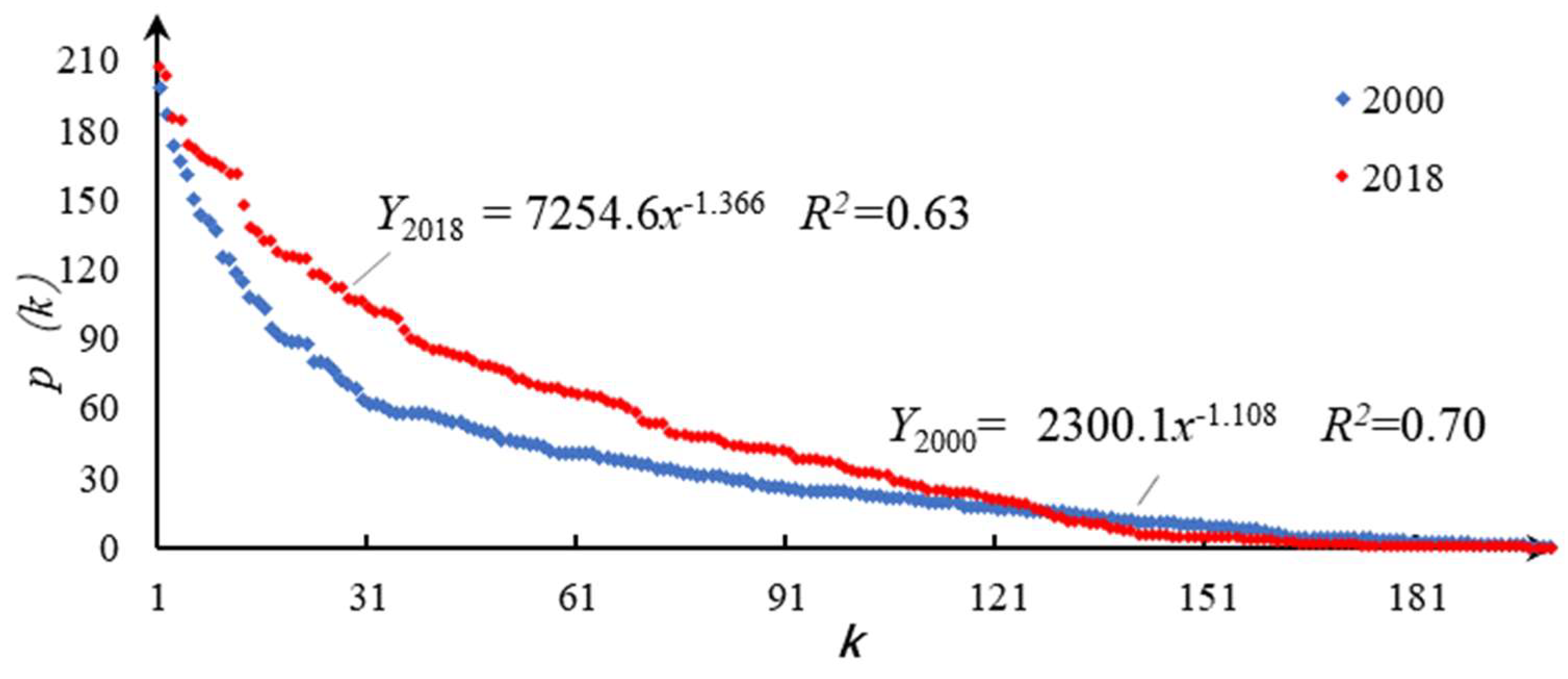
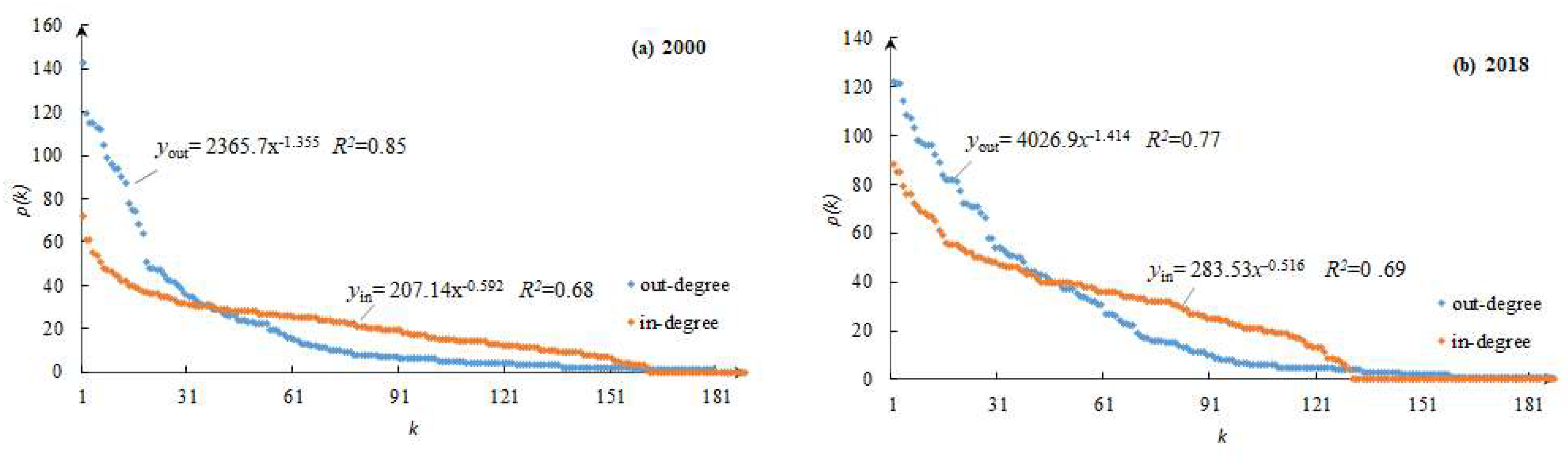
4.1.1. The Global Grain Network Has Scale-Free Properties

From the degree distribution maps of the global grain network in 2000 and 2018 (Figure 1), the degree distribution of the global grain network presents a “long tail” feature. This means that a few nodes have high degree values, whereas most have small and similar degree values. Power function fitting was conducted for the distribution in 2000 and 2018, and both passed the significance test, confirming that the degree distribution of the global grain network followed the power-law distribution, with significant heterogeneity among nodes, which was in accordance with the scale-free characteristics of the network. However, compared with that in 2000, the power ratio fitting value (R²) of the distribution curve in 2018 decreased, indicating that the scale-free characteristics of the global grain network weakened and the heterogeneity of nodes decreased. Moreover, R² of the power function of the out-degree distribution was greater than that of the in-degree distribution in 2000 and 2018 (Figure 2), indicating that the heterogeneity of the out-degree was greater than that of the in-degree.

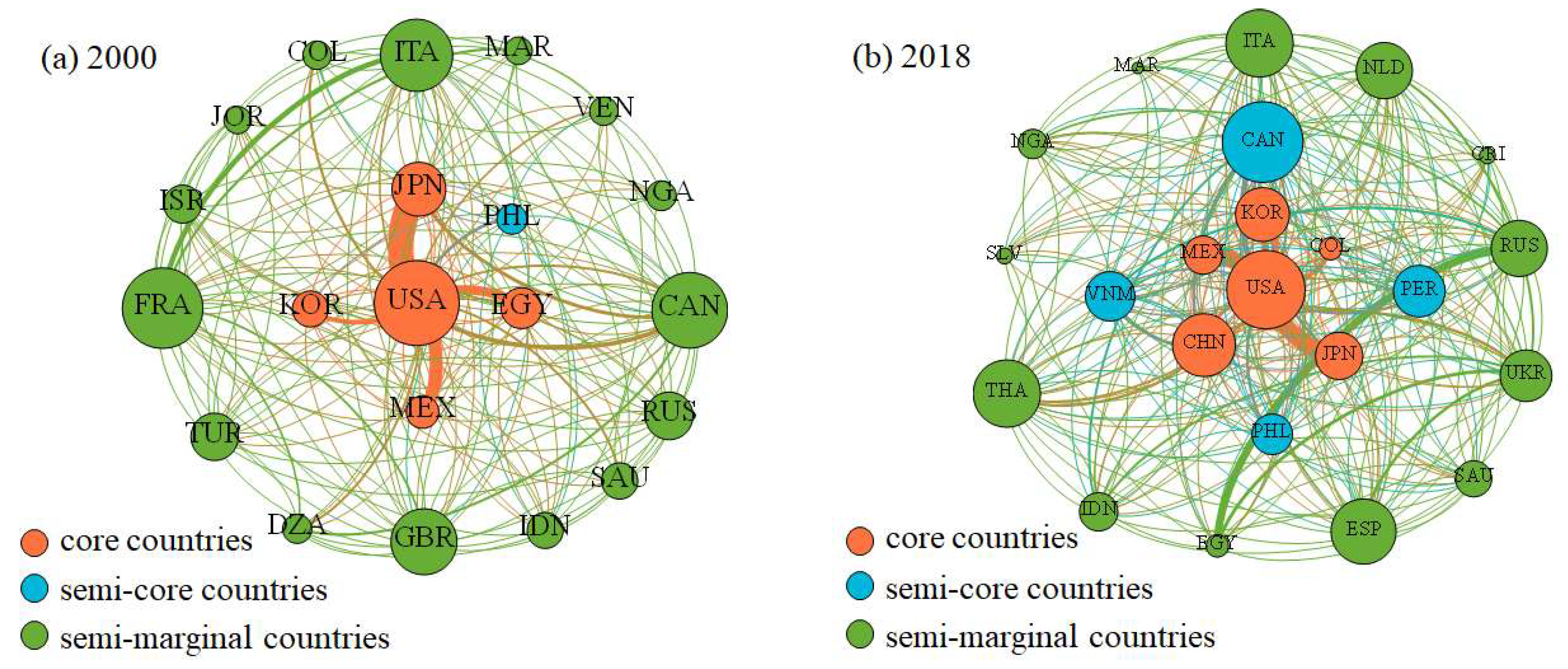
4.1.2. The Global Grain Network Presents a Significant “Core-Periphery” Structure

Figure 3 shows that the global grain network exhibits a significant “core-periphery” structure. In 2000, the core countries included the United States, Japan, Mexico, Egypt, and South Korea. The Philippines was the only semi-core country. The semi-marginal countries included 15 countries: the Philippines, Saudi Arabia, Algeria, Italy, Colombia, Canada, Venezuela, Nigeria, Israel, Russia, and Turkey. The remaining 175 countries were marginal. In 2018, the core periphery of the global grain network became more hierarchical because the number of core and semi-core countries increased and the number of semi-peripheral and peripheral countries decreased. In 2018, the core countries of the global grain network included the United States, Japan, Mexico, Egypt, the Republic of Korea, and Colombia. The semi-core countries included Venezuela, the Philippines, Peru, and Canada. There were 13 semi-marginal countries including Saudi Arabia, Egypt, Indonesia, Spain, Thailand, Ukraine, Italy, Nigeria, Russia, and the Netherlands. The number of peripheral countries was 173 (

Table 2. Quantitative of the four types of countries in the “core-periphery” structure in 2000 and 2018.

Year	Core Countries	Semi-Core Countries	Semi-Marginal Countries	Marginal Countries
2010	5	1	15	175
2018	6	4	13	173

).

4.2. Node Features

4.2.1. Heterogeneity of the Out-Degree Nodes

The out-degree indicates the number of node egress relationships. Taking 2000 data as a reference and using the natural breaks (Jenks) method, the output degree was divided into five grade types with 12, 29, 51, and 99 as the thresholds. Generally, the number of countries with higher out-degree values increased, whereas those with lower out-degree values decreased. Figure 4b shows that in 2018, there were eight countries with the highest out-degree values including the United States, Argentina, France, Italy, India, Pakistan, China, and Thailand, whose output values were greater than 100. There was one country with the highest out-degree value in 2000. The higher out-degree values between 52 and 99 including Vietnam, Spain, Canada, the United Kingdom, Russia, Peru, Germany, Turkey, the Netherlands, Belgium, South Africa, Australia, and another 26 countries, with 15 more countries than in 2000. There were 27 countries with out-degree values between 30 and 51 in 2018 including Denmark, the Czech Republic, Myanmar, Mexico, Portugal, Indonesia, Philippines, Malaysia, Egypt, and Kazakhstan, with eight more countries than in 2000. There were 24 countries with out-degree values between 13 and 29 in 2018 including Saudi Arabia, Finland, Nigeria, Ireland, Israel, Slovenia, Colombia, Guyana, Sudan, Zambia, Uganda, and Laos, with four less countries than in 2000. The remaining 111 countries scored below 12, with 20 fewer countries than in 2000.

4.2.2. Heterogeneity of In-Degree Nodes

In-degree indicates the number of node-import relationships. Taking the data of 2000 as a reference and using the natural discontinuity method, the in-degree was divided into five grades with thresholds of 7, 19, 32, and 48. Similar to the out-degree’s characteristics, the number of higher in-degree value countries increased, whereas the number of lower in-degree countries decreased. As shown in Figure 4d, 29 countries had the highest in-degree values between 49 and 99 in 2018 including France, Canada, Germany, the United States, the Netherlands, and Spain. Compared with 2000, there were 23 more countries. There were 44 countries with higher in-degree values between 33 and 48 in 2018 including Japan, South Korea, Hungary, Thailand, Kuwait, Ukraine, Australia, Portugal, China, New Zealand, India, Nigeria, Indonesia, and Egypt. There were 27 more countries than in 2000. There were 36 countries with in-degree values between 20 and 23 in 2018 including Uganda, Zambia, Zimbabwe, Burkina Faso, Latvia, Brazil, Colombia, and Peru, with a decrease of 23 countries compared to 2000. Mexico, Ecuador, Paraguay, Uzbekistan, Cambodia, Afghanistan, and another 19 countries ranked fourth in terms of in-degree with in-degree values ranging between 8 and 19. This is 39 fewer countries than in 2000. The remaining 68 countries including Laos, Iran, Ethiopia, Guinea, Jamaica, Gabon, Libya, Haiti, and Bahamas had an in-degree values below 7, which is 18 more countries than in 2000.

5. Driving Factor for the Evolution of the Global Grain Networks

5.1. Results of QAP Model Regression

Table 3. Results of QAP regression.

Indicators	2000	2018
LnRESij	0.05549 ** (6)	0.07321 ** (5) ↑
LnDISij	0.49405 ** (1)	0.40154 ** (1) ↓
CONij	0.06416 ** (5)	0.08368 ** (4) ↑
LnECOij	0.34524 ** (2)	0.38982 ** (2) ↑
LnPOLij	−0.12001 ** (3)	−0.17706 ** (3) ↑
RTAij	0.07089 ** (4)	0.04597 ** (6) ↓
CULij	−0.01824 ** (7)	−0.01047 ** (7) ↓
R2	0.886	0.877
AJ-R2	0.886	0.877
Model’s significance	p < 0.001	p < 0.001
Observation items	38,220	38,220

Note: ** represents p < 0.01; The absolute value ranking of regression coefficients is in parentheses (the same below); ”↑” and “↓” respectively indicate that the absolute value of the regression coefficient of variables in 2018 increased or decreased compared with that in 2000.

presents a summary that QAP regression models passed the 1% significance test in both 2000 and 2018, and the goodness of fit of the 2000 and 2018 models were 88.61% and 87.70%, respectively, indicating that the models had high explanatory power. QAP regression analysis results indicate that the resources endowment difference, the difference of geographical approaches, economic development, the free trade agreement, and the national comprehensive management ability between 2000 and 2018 had a significantly positive impact on the global grain network evolution, whereas social and cultural similarity had a significantly negative impact on the global grain network evolution. Moreover, the driving intensity of geographical distance, national comprehensive governance capacity, and free trade agreement decreased significantly. In 2018, the elasticity coefficient of these two factors decreased by 9.25%, 5.71%, and 2.49% compared with 2000. The driving intensity of the resource endowment difference, land border difference, economic development difference as well as cultural similarity increased, and the elastic coefficients of the four factors increased by 1.77%, 1.95%, 4.46%, and 0.78%, respectively, in 2018.

According to the classical gravity model theory, the longer the distance between the two countries, the weaker the trade links. However, our results indicate that in 2000 and 2018, the geographical distance had a positive impact on the formation of food trade links, and countries with greater distance are more likely to form trade links. This result is not consistent with the expectations, reflecting the uniqueness of food trade. Grain production has significant regional characteristics, and strongly depends on natural conditions. Countries in close proximity may have similar natural conditions, similar resource endowments, and similar regional grain production structures, which could hinder the formation of close grain trade links. In contrast, differences in natural conditions and the production structure between countries far away promote them to adjust the surplus or shortage through food trade as well as to adjust variety. For instance, in the global grain network, the larger volume of trading partners is long-distance such as China and the U.S., the EU and the U.S., Brazil and China as well as India and the U.S. [37]. However, compared with 2000, the regression coefficient of the geographical distance factor decreased in 2018, mainly because of the improvement in the modern ocean transportation system. Thus, the freight cost was significantly reduced and the impact of geographical distance on grain trade was reduced.

The grain trade had a significant “boundary effect.” QAP regression results indicate that land border had a positive effect on the formation of food trade links in both 2000 and 2018, and the coefficient showed an increasing trend. That is, countries bordering on land have closer food trade links, and the effect is increasing. As neighbors on land have been close for a long time, their public opinion is similar, mutual trust is high, and trade is more frequent. Because railway transportation is highly flexible and has a lower transit time than ocean transportation, neighboring countries on land often take advantage of the geographical benefits to promote grain trade through border ports and land transportation facilities. For instance, in recent years, China has maintained increasingly close food trade ties with its neighbors such as Russia, Pakistan, and Vietnam. Additionally, the United States has maintained close food trade ties with its land neighbor, Mexico, for a long time.

The level of economic development had a positive effect on the evolution of the grain trade network shown by a statistical significance test of 1%, and the influence coefficient showed an increasing trend. Countries with larger differences in economic development levels had a closer grain trade relationship. Generally, international grain trade mainly occurs between high-income and low-income countries. High-income countries are usually net grain export regions [61], whereas slow-income countries have maintained a consistent trend in net food imports. With a high degree of mechanization and a high per capita grain output, high-income countries such as the United States, Canada, Australia, and France, mainly export grain. Most low-income countries are in the process of transforming from plant-based food consumption to animal-based food consumption structures, and their food consumption increases rigidly. Their domestic food cannot meet the demand because of low productivity, and they have to rely on imports for food consumption.

The difference in political attributes had a negative impact on food trade, which passed the statistical significance test of 1%. Countries with smaller differences in national governance capacity had closer bilateral food trade links. Compared with 2010, the absolute value of the influence coefficient of national comprehensive governance capacity on the grain trade network exhibited an increasing trend in 2018.

The impact of resource endowment differences on the grain trade network passed the statistical significance test of 1%, indicating a positive influence, and the coefficient showed an increasing trend. The resource endowment difference is still an important factor affecting food trade. Under the condition of existing technology, food production depends highly on natural resources, specifically land resources. The greater the difference in per capita cultivated land resources between countries, the greater the bilateral trade value. As global arable land decreases and land scarcity increases, differences in resource endowments have an increasing impact on the global food trade.

Regional free trade agreements had a positive impact on grain networks using a statistical significance test of 1%, and the coefficient exhibited an increasing trend. Regional free trade agreements play a positive role in food trade. Signing bilateral free trade agreements has provided legal guarantees for bilateral economic and trade cooperation, reduced the cost of bilateral trade, and improved the level of trade facilitation. This contributed to the formation of a mutually beneficial situation to strengthen mutual food trade links.

Cultural similarity had a negative impact on the formation of food trade links using a statistical significance test of 1%. Countries with larger cultural differences had fewer bilateral food trade links, which is consistent with the expected result. Compared to 2000, the absolute value of the regression coefficient of cultural similarity exhibited a decreasing trend in 2018, but the relative ranking remained unchanged, ranking seventh among all influencing factors.

5.2. Robustness Test

To test the robustness of the QAP regression results, two methods of removing variables and randomly deleting samples were used to conduct the QAP regression analysis.

The results of the variable exclusion test in 2000 indicated that the QAP regression was relatively robust. After a variable was removed in 2000, the regression coefficient symbols of the remaining variables were consistent with the original QAP regression results, and all p values were less than 0.01 (

Table 4. Results of the variable exclusion test in 2000.

Indicators	Model 1	Model 2	Model 3	Model 4	Model 5	Model 6	Model 7
LnRESij		0.03832 **	0.04968 **	0.04802 **	0.04833 **	0.04230 **	0.05646 **
LnDISij	0.47128 **		0.45887 **	0.84713 **	0.64667 **	0.40053 **	0.49376 **
CONij	0.06190 **	0.05384 **		0.06720 **	0.07637 **	0.07440 **	0.06216 **
LnECOij	0.33375 **	0.75434 **	0.35725 **		0.27203 **	0.42114 **	0.34205 **
LnPOLij	−0.11397 **	−0.21721 **	−0.14651 **	−0.07978 **		−0.15989 **	−0.11660 **
RTAij	0.06427 **	0.03548 **	0.08411 **	0.09570 **	0.09461 **		0.06800 **
CULij	−0.01976 **	−0.01790 **	−0.01012 **	−0.01496 **	−0.01186 **	−0.00917 **
R2	0.884	0.877	0.882	0.880	0.882		0.885
AJ-R2	0.884	0.877	0.882	0.880	0.882		0.885
Model’s significance	p < 0.001	p < 0.001	p < 0.001	p < 0.001	p < 0.001		p < 0.001
Observation items	38,220	38,220	38,220	38,220	38,220	38,220	38,220

Note: ** represents p < 0.01.

). In addition, the results of the variable exclusion test in 2018 indicated that the QAP regression was robust. In 2018, the sign of the regression coefficient of cultural difference variables changed from negative to positive when only land border variables were excluded, but it was not significant. In addition, when other variables were removed, the regression coefficient symbols of the remaining variables were consistent with the original results, and all p values were less than 0.01 (

Table 5. Results of the variable exclusion test in 2018.

Indicators	Model 8	Model 9	Model 10	Model 11	Model 12	Model 13	Model 14
LnRESij		0.06357 **	0.06268 **	0.06527 **	0.06433 **	0.06855 **	0.07417 **
LnDISij	0.37491 **		0.32565 **	0.79360 **	0.65213 **	0.32627 **	0.40348 **
CONij	0.07974 **	0.07341 **		0.08931 **	0.10126 **	0.08728 **	0.08244 **
LnECOij	0.37053 **	0.73467 **	0.42639 **		0.25749 **	0.46590 **	0.38695 **
LnPOLij	−0.16940 **	−0.25540 **	−0.21765 **	−0.13003 **		−0.20275 **	−0.17506 **
RTAij	0.04010 **	0.01169 **	0.05806 **	0.08535 **	0.08339 **		0.04499 **
CULij	−0.01350 **	−0.01270 **	0.00001	−0.00373 **	−0.00314 **	−0.00801 **
R2	0.875	0.873	0.871	0.873	0.872	0.876	0.877
AJ-R2	0.875	0.873	0.871	0.873	0.872	0.876	0.877
Model’s significance	p < 0.001	p < 0.001	p < 0.001	p < 0.001	p < 0.001	p < 0.001	p < 0.001
Observation items	38,220	38,220	38,220	38,220	38,220	38,220	38,220

Note: ** represents p < 0.01.

).

The results were tested using a random deletion of the samples. Based on the original samples in 2000 and 2018, 20% of the samples were randomly excluded to obtain 35,910 and 35,532 samples. QAP regression was performed for the new samples. The new QAP regression results indicated that in 2000 and 2018, the regression symbols of all variables were consistent, and the p values were all less than 0.01, which passed the significance test at the 1% level (

Table 6. Results of randomly deleting samples test in 2000 and 2018.

Indicators	2000	2018
LnRESij	0.04142 **	0.06995 **
LnDISij	0.49925 **	0.39088 **
CONij	0.07030 **	0.08597 **
LnECOij	0.34104 **	0.39754 **
LnPOLij	−0.10828 **	−0.17727 **
RTAij	0.06927 **	0.04312 **
CULij	−0.02331 **	−0.00844 **
R2	0.886	0.878
AJ-R2	0.886	0.878
Model’s significance	p < 0.001	p < 0.001
Observation items	35,910	35,532

Note: ** represents p < 0.01.

). Therefore, the test results of the random deletion sample method also indicate that the empirical conclusion of this study is robust and credible.

6. Conclusions

This study constructed a weighted global grain network based on complex network theory using data from 2000 and 2018. First, we analyzed the topological properties of the evolution of the global grain network. We then investigated the evolution of the global grain trade and its spatial homogeneity for the years of 2000 and 2018 based on complex networks. Thereafter, we evaluated the impacts of six factors on the global food trade using the QAP model. We conclude that:

(1) The global grain network is scale-free. The distributions of degree, out-degree, and in-degree of the global grain network follow the power-law distribution. There was significant heterogeneity among nodes, and the heterogeneity of out-degree was greater than that of in-degree. There were eight countries with the highest output values greater than 100 including the United States, Argentina, France, Italy, India, Pakistan, China, and Thailand. There were 29 countries with the highest in-degree value between 49 and 99 including France, Canada, Germany, the United States, the Netherlands, and Spain.

(2) The global grain network has a significant core-periphery structure. The United States, Japan, Mexico, Egypt, South Korea, and Colombia are the core countries. Compared with 2000, the number of core and semi-core countries increased in 2018, whereas the number of semi-peripheral and peripheral countries decreased. This trend indicates that the “core-periphery” hierarchy of the global grain network is more obvious.

(3) Empirical research into trade network evolution mechanism with the six factors revealed several significant findings: (a) The geographical distance has a positive impact on the formation of food trade links in both 2000 and 2018, and countries with greater distance between them are more likely to form trade links. This is contrary to the classical gravity model theory, reflecting the uniqueness of the food trade. (b) Grain trade has significant “boundary effects.” Countries with land borders are more closely linked to the food trade, and this effect increases. (c) The level of economic development has a positive impact on the evolution of the grain trade network. Countries with larger differences in economic development have closer trade links, and the world grain trade mainly occurs between high-income and low-income countries. (d) The difference in resource endowment has a positive impact on the grain networks. Under existing technological conditions, food production is highly dependent on natural resources, specifically land resources. The scarcity of cultivated land increases with decreasing global cultivated land, and the impact of resource endowment differences on global food trade increases. (e) Regional free trade agreements have a positive impact on grain networks, and they play a positive role in food trade. In contrast, cultural similarity and differences in politics attributes have a negative impact on the formation of food trade links.

This study contributes to the literature by first addressing a gap in the global grain network research that focuses on structural and topological characteristics without considering its influencing factors. Second, the influence of geographical distance on grain trade is in contrast to the classical gravity model, which reflects the uniqueness of the food trade. Third, this study expands the application of the QAP model to the grain trade sector. In addition, this study can provide policymakers with a basis for the development of timely grain export and import strategy adjustments and policy-making processes.

There are several potential directions for future research. First, the impact of ocean liner transportation, tariff rates, currency interest rates, urbanization rates, and other factors on the global food trade should be considered. Second, innovative models such as the temporal exponential random graph model (TERGM) may be used to observe the endogenous structural and relational embeddedness effects. Third, it is necessary to add more cross-sectional data and improve the time resolution to observe more details of the variability for the 2000–2018 period in future research. Last, but not least, to explore the impacts of climate change on grain production and trade patterns. Global climate changes have multiple implications for the global food system by affecting food production, processing, packaging, storage, food prices, and retailing [62]. For example, climate change is projected to rise agriculture prices [63,64]. According to the Intergovernmental Panel on Climate Change (IPCC) global agricultural prices could increase up to 29% from the current levels by 2050 [65], which will aggravate financial burdens for food acquisition, particularly for net-importing countries [64]. Moreover, due to future climate change, many countries such as China [66], the United States [65], Bangladesh, and Myanmar [67] will suffer from decreases in crop production, while increases in precipitation and temperature will increase the yields and exports of wheat and rice in Kazakhstan [68]. The heterogeneous impacts of climate change across the world will change the relative competitive advantages in agricultural production, leading to significant adjustments of global grain trade patterns, and countries may experience the heterogeneous economic consequences depending on the position and the nodal relationship of each country in the global agricultural trade network [63]. Thus, the precise simulation of future changes in grain production and trade has important implications for stabilizing the international grain market and ensure food security.

References

1. Godfray, H.C.J.; Beddington, J.R.; Crute, I.R.; Haddad, L.; Lawrence, D.; Muir, J.F.; Pretty, J.; Robinson, S.; Thomas, S.M.; Toulmin, C. Food Security: The Challenge of Feeding 9 Billion People. Science 2010, 327, 812–818. [Google Scholar] [CrossRef] [Green Version]
2. Rosegrant, M.W.; Cline, S.A. Global Food Security: Challenges and Policies. Science 2003, 302, 1917–1919. [Google Scholar] [CrossRef] [PubMed] [Green Version]
3. Porkka, M.; Kummu, M.; Siebert, S.; Varis, O. From Food Insufficiency towards Trade Dependency: A Historical Analysis of Global Food Availability. PLoS ONE 2013, 8, e82714. [Google Scholar] [CrossRef] [Green Version]
4. Puma, M.; Bose, S.; Chon, S.Y.; Cook, B.I. Assessing the Evolving Fragility of the Global Food System. Environ. Res. Lett. 2015, 10, 24007. [Google Scholar] [CrossRef]
5. D’Odorico, P.; Carr, J.; Laio, F.; Ridolfi, L.; Vandoni, S. Feeding Humanity through Global Food Trade. Earth Future 2014, 2, 458–469. [Google Scholar] [CrossRef]
6. Matthews, A. Trade Rules, Food Security and the Multilateral Trade Negotiations. Eur. Rev. Agric. Econ. 2014, 41, 511–535. [Google Scholar] [CrossRef] [Green Version]
7. Gephart, J.A.; Pace, M. Structure and Evolution of the Global Seafood Trade Network. Environ. Res. Lett. 2015, 10, 125014. [Google Scholar] [CrossRef] [Green Version]
8. Dupas, M.-C.; Halloy, J.; Chatzimpiros, P. Time Dynamics and Invariant Subnetwork Structures in the World Cereals Trade Network. PLoS ONE 2019, 14, e0216318. [Google Scholar] [CrossRef] [Green Version]
9. Macdonald, G.K.; Brauman, K.; Sun, S.; Carlson, K.M.; Cassidy, E.S.; Gerber, J.; West, P. Rethinking Agricultural Trade Relationships in an Era of Globalization. BioScience 2015, 65, 275–289. [Google Scholar] [CrossRef]
10. Duan, J.; Xu, Y.; Jiang, H. Tradevulnerability Assessment in the Grain-Importing Countries: A Case Study of China. PLoS ONE 2021, 16, e0257987. [Google Scholar] [CrossRef]
11. FAO. World Food and Nutrition Press Security: Report. 2019. Available online: www.fao.org/home/search/en?Page=0&category=publications (accessed on 25 October 2020).
12. Foley, J.A.; Ramankutty, N.; Brauman, K.; Cassidy, E.S.; Gerber, J.; Johnston, M.; Mueller, N.D.; O’Connell, C.; Ray, D.; West, P.; et al. Solutions for a Cultivated Planet. Nat. Cell Biol. 2011, 478, 337–342. [Google Scholar] [CrossRef] [Green Version]
13. Crist, E.; Mora, C.; Engelman, R. The Interaction of Human Population, Food Production, and Biodiversity Protection. Science 2017, 356, 260–264. [Google Scholar] [CrossRef] [PubMed]
14. Herzberger, A.; Chung, M.G.; Kapsar, K.; Frank, K.A.; Liu, J. Telecoupled Food Trade Affects Pericoupled Trade and Intracoupled Production. Sustainability 2019, 11, 2908. [Google Scholar] [CrossRef] [Green Version]
15. Serrano, M. Ángeles; Boguñá, M. Topology of the World Trade Web. Phys. Rev. E 2003, 68, 015101. [Google Scholar] [CrossRef] [PubMed] [Green Version]
16. Fagiolo, G.; Reyes, J.; Schiavo, S. World-Trade Web: Topological Properties, Dynamics, and Evolution. Phys. Rev. E 2009, 79, 036115. [Google Scholar] [CrossRef] [Green Version]
17. He, Z.; Yang, Y.; Liu, Y.; Jin, F. Characteristics of Evolution of Global Energy Trading Network and Relationships Between Major Countries. Prog. Geogr 2019, 38, 1621–1632. [Google Scholar] [CrossRef]
18. Kitamura, T.; Managi, S. Driving Force and Resistance: Network Feature in Oil Trade. Appl. Energy 2017, 208, 361–375. [Google Scholar] [CrossRef]
19. Hou, W.; Liu, H.; Wang, H.; Wu, F. Structure and Patterns of the International Rare Earths Trade: A Complex Network Analysis. Resour. Policy 2018, 55, 133–142. [Google Scholar] [CrossRef]
20. Sui, G.; Zou, J.; Wu, S.; Tang, D. Comparative Studies on Trade and Value-Added Trade Along the “Belt and Road”: A Network Analysis. Complexity 2021, 2021, 3994004. [Google Scholar] [CrossRef]
21. Dong, C.; Yin, Q.; Lane, K.J.; Yan, Z.; Shi, T.; Liu, Y.; Bell, M. Competition and Transmission Evolution of Global Food Trade: A Case Study of Wheat. Phys. A Stat. Mech. Appl. 2018, 509, 998–1008. [Google Scholar] [CrossRef]
22. Shutters, S.T.; Muneepeerakul, R. Agricultural Trade Networks and Patterns of Economic Development. PLoS ONE 2012, 7, e39756. [Google Scholar] [CrossRef]
23. Cai, H.; Song, Y. The state’s Position in International Agricultural Commodity Trade. China Agric. Econ. Rev. 2016, 8, 430–442. [Google Scholar] [CrossRef]
24. Wang, X.; Niu, S.W.; Qiang, W.L.; Liu, A.M.; Cheng, S.K.; Qiu, X. Trade Network of Global Agricultural Products Weighted by Physical and Value Quantity. Econ. Geogr. 2019, 39, 164–173. [Google Scholar] [CrossRef]
25. Fan, Y.; Ren, S.; Cai, H.; Cui, X. The state’s Role and Position in International Trade: A Complex Network Perspective. Econ. Model. 2014, 39, 71–81. [Google Scholar] [CrossRef]
26. Chen, W.-Q.; Graedel, T.E.; Nuss, P.; Ohno, H. Building the Material Flow Networks of Aluminum in the 2007 U.S. Economy. Environ. Sci. Technol. 2016, 50, 3905–3912. [Google Scholar] [CrossRef]
27. Nuss, P.; Chen, W.-Q.; Ohno, H.; Graedel, T.E. Structural Investigation of Aluminum in the U.S. Economy Using Network Analysis. Environ. Sci. Technol. 2016, 50, 4091–4101. [Google Scholar] [CrossRef] [PubMed]
28. Nie, C.L.; Jiang, H.N.; Duan, J. Spatial Pattern Evolution of Global Grain Trade Network since the 21st Century. Econ. Geogr. 2021, 41, 119–127. [Google Scholar] [CrossRef]
29. Wu, Z.; Cai, H.; Zhao, R.; Fan, Y.; Di, Z.; Zhang, J. A Topological Analysis of Trade Distance: Evidence from the Gravity Model and Complex Flow Networks. Sustainability 2020, 12, 3511. [Google Scholar] [CrossRef]
30. Anderson, J.E.; Van Wincoop, E. Gravity with Gravitas: A Solution to the Border Puzzle. Am. Econ. Rev. 2003, 93, 170–192. [Google Scholar] [CrossRef] [Green Version]
31. Mizik, T. Agri-Food Trade Competitiveness: A Review of the Literature. Sustainability 2021, 13, 11235. [Google Scholar] [CrossRef]
32. Tadesse, B.; White, R. Does Cultural Distance Hinder Trade in Goods? A Comparative Study of Nine OECD Member Nations. Open Econ. Rev. 2010, 21, 237–261. [Google Scholar] [CrossRef]
33. Shi, B.Z. Cultural Identification and International Trade. J. World Econ. 2016, 39, 78–97. [Google Scholar]
34. Feng, L.; Xu, H.; Wu, G.; Zhang, W. Service Trade Network Structure and Its Determinants in the Belt and Road Based on the Temporal Exponential Random Graph Model. Pac. Econ. Rev. 2021, 26, 617–650. [Google Scholar] [CrossRef]
35. Serrano, R.; Pinilla, V. Causes of World Trade Growth in Agricultural and Food Products, 1951–2000: A Demand Function Approach. Appl. Econ. 2010, 42, 3503–3518. [Google Scholar] [CrossRef] [Green Version]
36. Manger, M.S.; Pickup, M.A.; Snijders, T.A.B. A Hierarchy of Preferences. J. Confl. Resolut. 2012, 56, 853–878. [Google Scholar] [CrossRef]
37. Anderson, J.E.; Marcouiller, D. Insecurity and the Pattern of Trade: An Empirical Investigation. Rev. Econ. Stat. 2002, 84, 342–352. [Google Scholar] [CrossRef] [Green Version]
38. Wang, J.-Y.; Dai, C.; Zhou, M.-Z.; Liu, Z.-J. Research on Global Grain Trade Network Pattern and Its Influencing Factors. J. Nat. Resour. 2021, 36, 1545–1556. [Google Scholar] [CrossRef]
39. McCallum, J. National Borders Matter: Canada-U.S. Regional Trade Patterns. Am. Econ. Rev. 1995, 85, 615–623. [Google Scholar]
40. Kimura, F.; Lee, H.-H. The Gravity Equation in International Trade in Services. Rev. World Econ. 2006, 142, 92–121. [Google Scholar] [CrossRef]
41. Lee, J. Network Effects on International Trade. Econ. Lett. 2012, 116, 199–201. [Google Scholar] [CrossRef]
42. Gani, A.; Clemes, M.D. Modeling the Effect of the Domestic Business Environment on Services Trade. Econ. Model. 2013, 35, 297–304. [Google Scholar] [CrossRef]
43. Huang, S.Y.; Gou, W.S.; Cai, H.B.; Li, X.M.; Chen, Q.H. Effects of Regional Trade Agreement to Local and Global Trade Purity Relationships. Complexity 2020, 2987217. [Google Scholar] [CrossRef]
44. Watkins, M.H.; Linder, S.B. An Essay on Trade and Transformation. Can. J. Econ. Political Sci. 1963, 29, 121. [Google Scholar] [CrossRef]
45. Ma, J.; He, C. Structure and Change of International Trade Network of Intermediate Goods: From the Perspective of Trade Costs. Prog. Geogr 2019, 38, 1607–1620. [Google Scholar] [CrossRef]
46. Chen, Y.; Li, E. Spatial Pattern and Evolution of Cereal Trade Networks Among the Belt and Road Countries. Prog. Geogr 2019, 38, 1643–1654. [Google Scholar] [CrossRef]
47. Davis, L.S.; Abdurazokzoda, F. Language, Culture and Institutions: Evidence from a New Linguistic Dataset. J. Comp. Econ. 2016, 44, 541–561. [Google Scholar] [CrossRef]
48. Walker, S. Cultural Barriers to Market Integration: Evidence from 19th Century Austria. J. Comp. Econ. 2018, 46, 1122–1145. [Google Scholar] [CrossRef]
49. Yang, W.L.; Du, D.B.; Ma, Y.H.; Jiao, M.Q. Network Structure and Proximity of the Trade Network in the Belt and Road Region. Geogr. Res. 2018, 37, 2218–2235. [Google Scholar]
50. Carrère, C. Revisiting the Effects of Regional Trade Agreements on Trade Flows with Proper Specification of the Gravity Model. Eur. Econ. Rev. 2006, 50, 223–247. [Google Scholar] [CrossRef] [Green Version]
51. Ghosh, S.; Yamarik, S. Are Regional Trading Arrangements Trade Creating? An Application of Extreme Bounds Analysis. J. Int. Econ. 2004, 63, 369–395. [Google Scholar] [CrossRef]
52. Magee, C.S. New Measures of Trade Creation and Trade Diversion. J. Int. Econ. 2008, 75, 349–362. [Google Scholar] [CrossRef]
53. Ding, S.H.; He, S.Q. Analysis on the Efficiency and Influence Factors of China’s Agricultural Products Export to the Five Central Asian Countries. Int. Bus. 2019, 13–24, 5. [Google Scholar] [CrossRef]
54. Zhen, J.; Wang, X.M. Potential and Influencing Factors of Agricultural Trade Among RCEP members—Empirical Analysis Based on Stochastic Frontier Gravity Model. Xinjiang State Farms Econ. 2019, 8, 28–36, 64. [Google Scholar]
55. Dalin, C.; Konar, M.; Hanasaki, N.; Rinaldo, A.; Rodriguez-Iturbe, I. Evolution of the Global Virtual Water Trade Network. Proc. Natl. Acad. Sci. USA 2012, 109, 5989–5994. [Google Scholar] [CrossRef] [PubMed] [Green Version]
56. Geng, J.-B.; Ji, Q.; Fan, Y. A Dynamic Analysis on Global Natural Gas Trade Network. Appl. Energy 2014, 132, 23–33. [Google Scholar] [CrossRef]
57. Borgatti, S.; Everett, M.G. Models of core/Periphery Structures. Soc. Netw. 2000, 21, 375–395. [Google Scholar] [CrossRef]
58. Zheng, L.; Liu, Y.; Liu, W.D. Globalization and Regionalizationof Complete Auto’s and Auto parts’ trade. Sci. Geogr. Sin. 2016, 36, 662–670. [Google Scholar] [CrossRef]
59. Elliott, A.; Chiu, A.; Bazzi, M.; Reinert, G.; Cucuringu, M. Core–periphery Structure in Directed Networks. Proc. R. Soc. A Math. Phys. Eng. Sci. 2020, 476, 20190783. [Google Scholar] [CrossRef]
60. Xu, H.; Cheng, L. The QAP Weighted Network Analysis Method and Its Application in International Services Trade. Phys. A Stat. Mech. Appl. 2016, 448, 91–101. [Google Scholar] [CrossRef]
61. Feng, Z.M.; Zhao, X.; Yang, Y.Z. Evolutionary Trends of World Cereal Trade in Recent 50 Years from a View of Spatial-Temporal Patternsand Regional Differences. Resour. Sci. 2010, 32, 2–10. [Google Scholar]
62. Molly, E.B.; Edward, R.C.; Kathryn, L.G.; Keith, W.; Christopher, C.F.; Witsanu, A.; Peter, B.; Lawrence, B. Do Markets and Trade Help or Hurt the Global Food System Adapt to Climate change? Food Policy 2017, 68, 154–159. [Google Scholar] [CrossRef] [Green Version]
63. Lee, H.-L.; Lin, Y.-P.; Petway, J.R. Global Agricultural Trade Pattern in A Warming World: Regional Realities. Sustainability 2018, 10, 2763. [Google Scholar] [CrossRef] [Green Version]
64. Janssens, C.; Havlík, P.; Krisztin, T.; Baker, J.; Frank, S.; Hasegawa, T.; Leclère, D.; Ohrel, S.; Ragnauth, S.; Schmid, E.; et al. Global Hunger and Climate Change Adaptation through International Trade. Nat. Clim. Chang. 2020, 10, 829–835. [Google Scholar] [CrossRef] [PubMed]
65. Kunimitsu, Y.; Sakurai, G.; Iizumi, T. Systemic Risk in Global Agricultural Markets and Trade Liberalization under Climate Change: Synchronized Crop-Yield Change and Agricultural Price Volatility. Sustainability 2020, 12, 10680. [Google Scholar] [CrossRef]
66. Xie, W.; Huang, J.; Wang, J.; Cui, Q.; Robertson, R.; Chen, K. Climate Change Impacts on China’s Agriculture: The Responses from Market and Trade. China Econ. Rev. 2020, 62, 101256. [Google Scholar] [CrossRef]
67. Wu, F.; Wang, Y.; Liu, Y.; Liu, Y.; Zhang, Y. Simulated Responses of Global Rice Trade to Variations in Yield under Climate Change: Evidence from Main Rice-Producing Countries. J. Clean. Prod. 2021, 281, 124690. [Google Scholar] [CrossRef]
68. Yu, X.; Luo, H.; Wang, H.; Feil, J.-H. Climate Change and Agricultural Trade in Central Asia: Evidence from Kazakhstan. Ecosyst. Heal. Sustain. 2020, 6, 1766380. [Google Scholar] [CrossRef]
Figure 1. Distribution curve of node degree of the grain trade network.
Sustainability 14 00245 g001
Figure 2. Distribution curve of in-degree and out-degree of the grain trade network in 2000 (a) and 2018 (b).
Sustainability 14 00245 g002
Figure 3. The “core-periphery” structures of the global grain trade network in 2000 (a) and 2018 (b).
Sustainability 14 00245 g003
Figure 4. Evolution of in-degree and out-degree nodes of the global grain trade network in 2000 and 2018. Note: (a) out-degree in 2000; (b) in-degree in 2000; (c) out-degree in 2018; (d) in-degree in 2018. The gray line represents the trade flow among nodes. The thicker the line, the greater the trade flow.
Sustainability 14 00245 g004