Archimedes Optimization Algorithm Based Selective Harmonic Elimination in a Cascaded H-Bridge Multilevel Inverter

Abstract

This paper presents the Archimedes optimization algorithm to eliminate selective harmonics in a cascaded H-bridge (CHB) multilevel inverter (MLI). The foremost objective of the selective harmonic elimination (SHE) is to eliminate lower order harmonics by finding the optimal switching angle combination which minimizes the objective function containing Total Harmonic Distortion (THD) and other specific harmonic terms. Consequently, the THD is also reduced. In this study, a recently proposed metaheuristic technique named the Archimedes optimization algorithm (AOA) is used to determine the optimal angles corresponding to the 5, 7 and 9 level CHB-MLI. AOA involves equations related to a physical law, the Archimedes Principle. It is based on the idea of a buoyant force acting upward on a body or object that is partially or completely submerged in a fluid, and the upward force is related to the weight of the fluid displaced. This optimization technique has been implemented on CHB-MLI to generate various level outputs, simulated on MATLAB™ R2021a version environment software. The simulation results reveal that AOA is a high-performance optimization technique in terms of convergence speed and exploitation-exploration balance and is well-suited to the solution of the SHE problem. Furthermore, the laboratory validated the simulation result on a hardware setup using DSP-TMS320F28379D.

1. Introduction

Renewable energy such as wind and solar energy provides dc power that can be converted into ac power by an inverter. However, this generated power cannot be directly utilized for application in industry because it is very low. To overcome these problems, multilevel inverters are used for high power applications such as electric drives, active filters, frequency link systems, utility interfaces for renewable energy resources, induction motor control, voltage regulation, reactive power compensation, high-voltage system interconnections and variable speed motor drives [1]. Multi-Level Inverters (MLIs) can produce staircase sinusoidal-like output. The name “multilevel” refers to the output waveform, which resembles steps and hence forms levels, resulting in lower THD and in the desired sinusoidal waveform. Increasing the number of levels in the network topology will increase smoothness and thus reduce the harmonic distortion [2]. The major features of MLIs are the transformer-less structure, minimal switching losses and less stress on power semiconductors.

Depending upon the number of dc sources, capacitors, diodes and semiconductor switches used in the circuit, there may be numerous classifications of the inverters. Multilevel inverters are of three basic kinds mentioned in the literature: Diode-Clamped MLI, Cascaded H-bridge MLI and Flying-Capacitor MLI [2,3,4,5,6,7,8,9,10,11,12,13,14,15]. The cascaded H-bridge (CHB) is the most commonly used MLI due to its simple and modular structure and low component count [3]. This modular design allows for easy extension of the output voltage levels without increasing the power circuit’s complexity or requiring extra clamping diodes or voltage balancing capacitors. The topology of the cascaded H-bridge is composed of a S number of single-phase full-bridge inverters connected in series to create a (2S + 1) number of levels [4].

One of the most challenging issues with the MLI is reducing harmonics. Essentially, several control strategies may be used to improve the output quality and the performance of MLIs. A variety of strategies have been developed according to modulation and control for multilevel converters including space vector modulation (SVM), selective harmonic elimination pulse width modulation (SHE-PWM) and sinusoidal pulse width modulation (SPWM). Fundamental frequency and high frequency switching techniques can be used to classify these technologies. Fundamental frequency switching techniques such as selective harmonic elimination (SHE) and space vector modulation have attracted a lot of interest in recent years because they increase power conversion efficiency, reduce power losses, and lower prices [5]. SPWM introduces increased switching losses and harmonics at higher frequencies. Computational intricacy is a significant disadvantage of SVM. Consequently, it can only be used in real-time applications. The switching losses are decreased using the staircase modulation technique. In the case of staircase modulation, a variety of strategies have been described to reduce lower order harmonics in CHB-MLI. In recent years, the SHE-PWM has been an extensively used technique for removing lower order harmonics from the output voltage of the inverter. SHE-PWM techniques perform better than the other modulation methods in several ways, including an acceptable performance with direct control over output waveform harmonics and the ability to leave triple harmonics uncontrolled to take advantage of circuit topology in three-phase systems [6]. The concept of SHE has recently attracted a lot of interest. It can minimize the harmful lower harmonics in the output voltage waveforms. The nonlinear transcendental equations of the SHE control algorithm have complex solutions, making it difficult to use [6]. As a result, these strategies are ineffective when dealing with a large number of switching angles. The degree of polynomials in the equations increases as the number of harmonics to be eliminated increases, making it extremely difficult to solve them using existing methods. Furthermore, these algorithms are quite sensitive to initial predictions, and there is a significant risk of divergence, especially for greater numbers of levels [7].

To calculate the optimized firing angle, evolutionary techniques such as PSO (Particle Swarm Optimization), BA (Bee Algorithm), and GA (Genetic Algorithm) can be used to overcome the problem of iterative method and divergence chances [10,11,12]. The drawbacks of GA are its slow convergence speed, early convergence, and limited ability to perform local searches. In contrast to GA, PSO lacks evolution operators such as crossover and mutation. PSO rapidly converges to a nearly optimal solution. However, the main drawback of PSO is that it cannot fine-tune its velocity step size, resulting in the algorithm’s premature convergence. Ref. [13] demonstrated the superiority of the improved colonial competitive algorithm (ICCA) to GA and PSO in convergence rate. With regard to the convergence rate and precision, the GSA-based SHE approach showed significant improvements over GA in [15]. These techniques are easy to comprehend and implement. The Evolutionary algorithm employs a fitness function that takes into account both lower-order and fundamental harmonics of transcendental equations. The main purpose of the evolutionary algorithm is to minimize the fitness function in order to acquire the best firing angles. The ability of metaheuristic algorithms to provide improved approaches to popular optimization algorithms has become a major challenge for algorithm researchers in recent decades. The metaheuristic method is built on two pillars: inspiration and mathematical modeling. This goal is frequently achieved by employing strong mathematical models based on a compelling concept. These equations can also be solved well using neural networks (NN), Firefly algorithm (FFA), ant colony optimization (ACO), and fuzzy logic (FL). Ref. [16] introduces a new algorithm, the Crystal Structure Algorithm (CryStAl). Other approaches that are derivatives of the aforementioned ones can also be used. Each algorithm has its own set of advantages and disadvantages. Some algorithms require a long time to calculate and yield better results, and vice versa. However, there is always scope for improvement in terms of accuracy and convergence, allowing researchers to develop new optimization approaches for the SHE problem.

This paper utilizes a widely used test environment for experimentation and to evaluate the proposed AOA algorithm’s performance. Archimedes’ principle explains the law of buoyancy. It describes the relationship between an object submerged in water (fluid) and a buoyant force applied on it. As a result, an object’s buoyancy is affected by an upward force equal to the displaced fluid’s weight [17]. The object will sink if the weight of the object is greater than the displaced fluid weight. Otherwise, the object floats on the fluid (water) if the displaced fluid’s weight is equal to the object weight. In AOA, the objects immersed in the fluid are the population individual. The object has volume, acceleration and density, which plays a significant role in the objects buoyance force, which means that the fluid’s resultant net force is equal to zero. We found that the proposed approach is much more efficient with the ability to search globally when the AOA performance is examined by using a large testbed that includes both constrained engineering design challenges and unconstrained benchmark functions. To summarize, this study proposes a new population-based technique named AOA, which is based on the physics law known as Archimedes’ principle, to compete with this state-of-the-art and contemporary optimization algorithm as well as other physics-inspired methods. It is worth noting that the algorithm provided here maintains the perfect balance of exploitation and exploration. As a result of this feature, AOA is well suited to solve complicated problems. Because it maintains a population of solutions and analyzes a problem with many global optimum solutions, it is useful for optimization problems with many local optimal solutions. To identify the optimum global solution, a broad area must be searched. In this paper the implementation of AOA led to the elimination of lower order harmonics in Five-Level, Seven-Level and Nine-Level. The comparison between GA, DE and AOA has also been discussed. THD values for a range of modulation indexes were compared to confirm the superiority of AOA over DE and GA.

This paper constitutes eight sections in which Section 1 is the introduction. Section 2 describes the CHB-MLI whereas Section 3 provides the elementary idea of the Archimedes principle. The design and the framework of AOA are explained in Section 4. The idea of Selective harmonics elimination, and how AOA is implemented with SHE (Selective harmonic Elimination) in reducing the 5th harmonics, 5th and 7th harmonics, and 5th, 7th, and 11th harmonics are respectively removed from five-level, seven-level, and nine-level output, is described in Section 5. The simulation results are given in Section 6. The hardware results are discussed in Section 7, and the conclusion is presented in Section 8.

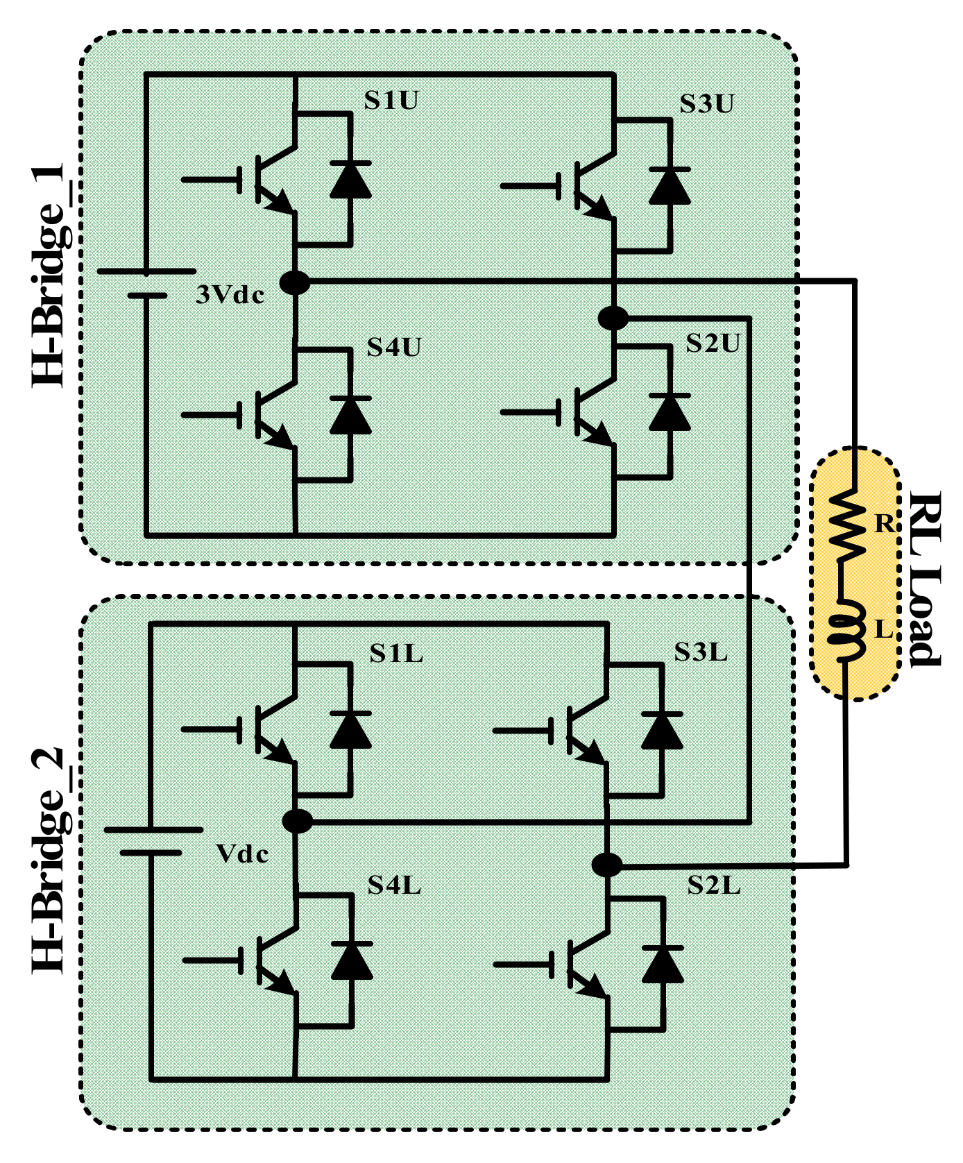
2. Cascaded H-Bridge Multilevel Inverter

The multi-level inverter was first proposed in 1975 as a diode clamped MLI. MLI has a staircase output voltage that resembles a sine wave. This stepped output waveform reduces the harmonics and enhances power quality. Higher number of output voltage levels lowers the THD, hence the losses corresponding to these harmonics are also reduced. The MLIs have been very popular in high and medium power applications such as flexible AC transmission systems (FACTS), industrial drives, solar photovoltaic system and power compensators. Reduced number of switches, low THD output voltage, improved power quality, low voltage stresses, good electromagnetic compatibility, lower switching frequency, and low common mode voltage are the attractive properties of MLI.

Researchers have emphasized compacting the inverter size without compromising the number of output voltage levels. This can be achieved by reducing the number of dc sources and switches. Numerous MLI topologies mentioned in the literature have been sorted into three major categories: Cascaded H-bridge (CHB) MLI, Flying Capacitor (FC) MLI and Diode Clamp (DC) MLI. The large number of capacitors in FC-MLI increases the volume and cost of the inverter. Moreover, regulating the capacitor voltage to the required value is challenging. An additional clamping diode is required in DC-MLI, and capacitor voltage balancing is difficult. The problem intensifies as the number of steps in the output voltage is increased. No clamping diode is required in CHB-MLI. The reliability, simplicity and modularity of the CHB-MLI topology make it preferable over others. Generally, two or more H-bridges are linked in a cascaded fashion to increase output voltage levels. Therefore, the number of dc voltage sources and switches are increased [2]. Consequently, the system complexity is increased. Each bridge with a separate source can produce an output voltage with three levels (−Vdc, +Vdc, and zero). CHB-MLI can either be asymmetrical or symmetrical depending on the voltage source combination ratio used in the system. In symmetrical CHB-MLI, voltage sources of equal magnitude are employed, while in asymmetrical CHB-MLI, voltage sources of unequal magnitude are used. 2(N−1) switches and (N−1)2 dc sources can generate N-level output. Sixteen switches and 4 dc sources are required to produce a 9-level output voltage in a symmetrical arrangement. With the same number of dc sources and switches, asymmetrical CHB-MLI can generate a higher number of output voltage levels using a different voltage combination ratio than symmetrical CHB-MLI. Figure 1 shows a Cascaded H-bride inverter employing two dc voltage sources. In a symmetrical configuration, only eight switches and two dc sources are required to produce nine-level output. Two cascaded H-bridges employing two sources and eight switches with source combination ratios of 1:1, 1:2 and 1:3 will produce an output voltage with five, seven and nine levels respectively [3].

3. Archimedes Principle

When an object (W₁) is partially or entirely submerged in a fluid, Archimedes’ principle asserts that an upward force is exerted by the fluid on the objects, which is equal to the weight of the fluid that the object displaced. Figure 2 depicts that when an object is submerged in fluid, it will undergo an upward movement, often called the buoyant force, which is equal to the fluid expelled (W₂) by the submerged object.

Assuming that in the same fluid, several objects are immersed, as illustrated in Figure 3, each attempting to reach equilibrium, the densities and volumes of the immersed items vary, which results in different accelerations. If the weight of the object is Wo which is equal to the buoyant force F_B, then the object will reach the Equilibrium state:

$$\begin{gathered} {\mathrm{F}}_{\mathrm{B}}=\mathrm{Wo} \\ {\mathsf{\rho }}_{\mathrm{B}}{\mathrm{V}}_{\mathrm{B}}{\mathrm{A}}_{\mathrm{B}}={\mathsf{\rho }}_{\mathrm{O}}{\mathrm{V}}_{\mathrm{O}}{\mathrm{A}}_{\mathrm{O}} \end{gathered}$$

(1)

where, $\mathsf{\rho }$ = Density, V = Volume, A = Acceleration or Gravity. Subscript B and O are for the fluid and immersed object respectively.

The equation can be rewritten as

$${\mathrm{A}}_{\mathrm{O}}=\frac{{\mathsf{\rho }}_{\mathrm{B}}{\mathrm{V}}_{\mathrm{B}}{\mathrm{A}}_{\mathrm{B}}}{{\mathsf{\rho }}_{\mathrm{O}}{\mathrm{V}}_{\mathrm{O}}}$$

(2)

If an additional force acts on the object, such as a collision among nearby objects (R), then in that condition the equilibrium state will be:

$$\begin{gathered} {\mathrm{F}}_{\mathrm{B}}=\mathrm{Wo} \\ {\mathrm{W}}_{\mathrm{B}}-{\mathrm{W}}_{\mathrm{R}}=\mathrm{Wo} \\ {\mathsf{\rho }}_{\mathrm{B}}{\mathrm{V}}_{\mathrm{B}}{\mathrm{A}}_{\mathrm{B}}-{\mathsf{\rho }}_{\mathrm{R}}{\mathrm{V}}_{\mathrm{R}}{\mathrm{A}}_{\mathrm{R}}={\mathsf{\rho }}_{\mathrm{O}}{\mathrm{V}}_{\mathrm{O}}{\mathrm{A}}_{\mathrm{O}} \end{gathered}$$

(3)

4. Archimedes Optimization Algorithm

AOA is an Algorithm which is based on population. Each individual of the population is converged in the proposed strategy. AOA, just like other population-based metaheuristic algorithms, begins the process of searching with a basic set of criteria. Random accelerations, volumes, and densities are used for the initial population of objects (possible solutions). During this point, each of the objects has a separate entity. In the fluid, its random position is likewise initialized. Subsequently, the AOA evaluates the starting population fitness. Until the termination condition is met the iterations are continued. At each iteration, the AOA changes the volume and density of each object. Based on the condition, the object’s acceleration is updated with the chances of colliding with any other nearby object. The new acceleration, volume and density are determined by the location of the object. The following is a full mathematical analysis of the steps involved in AOA, and a flowchart of the steps involved in AOA is also shown in Figure 4.

4.1. Algorithm Steps

This section introduces the mathematical formulation of AOA. It can theoretically be term as the global optimization algorithm because it encloses the two operations (a) exploitation operation and (b) exploration operation. The flow-chart of the proposed algorithm exhibits the evaluation of the population size, initialization of population and parameter updating. Mathematically, the detailed steps of the proposed AOA are as follows.

4.1.1. Initialization

In this step by the application of Equation (4) the position of all the objects is initialized:

$$\begin{gathered} {\mathrm{O}}_{\mathrm{I}}={\mathrm{lb}}_{\mathrm{i}}+\mathrm{rand}\times \left({\mathrm{ub}}_{\mathrm{i}}-{\mathrm{lb}}_{\mathrm{i}}\right) \\ \mathrm{i}=1,2,3,\dots ,\mathrm{N} \end{gathered}$$

(4)

where ${\mathrm{O}}_{\mathrm{I}}$ is the ith object in the population of N number of objects. ${\mathrm{ub}}_{\mathrm{i}}$ and ${\mathrm{lb}}_{\mathrm{i}}$ are the search space upper bounds and the lower bounds respectively.

$${\mathrm{den}}_{\mathrm{i}}=\mathrm{rand},{\mathrm{vol}}_{\mathrm{I}}=\mathrm{rand}$$

(5)

Initializing den (Density) and vol (Volume) for every Ith object using Equation (5), where D dimension vector randomly generates numbers among [0,1] and is indicated randomly. Using Equation (6) the acc (acceleration) of the ith object is finally initialized.

$$ac{c}_i=l{b}_i+rand\times (u{b}_i-l{b}_i)$$

(6)

The initial population is evaluated at this step, and the best fitness value object is selected. Allocate as acc_best, den_best, x_best, vol_best.

Volumes and Densities Update

By application of Equation (7), the object volume and density for the iteration t + 1 are updated.

$$\begin{gathered} de{n}_i^{t+1}=de{n}_i^t+rand\times \left(de{n}_{best}-de{n}_i^t\right) \\ vo{l}_i^{t+1}=vo{l}_i^t+rand\times \left(vo{l}_{best}-vo{l}_i^t\right) \end{gathered}$$

(7)

Here, rand is the uniformly distributed random number and den_best and vol_best are the best-associated density and volume with the best object found.

Density Factor and Transfer Operation

In the beginning, before the object collision occurs, each object tries to achieve equilibrium state after tenure. The AOA implements this state by acquiring a transfer operator (TF) responsible for transforming search from exploration to exploitation with the help of Equation (8).

$$TF=\exp \left(\frac{t-t_{max}}{Ma{x}_{iter}}\right)$$

(8)

while time extending until 1, the transfer TF gradually increases. Here Max_iter and t are maximum iterations and iteration numbers, respectively. Similarly, the AOA is assisted on global to local search by d density decreasing factor. Using Equation (9), it decreases with time.

$$d^{t+1}=\exp \left(\frac{t-t_{max}}{Ma{x}_{iter}}\right)-\left(\frac{t}{t_{max}}\right)$$

(9)

Here, d^t+1 decreases with time, allowing convergence in a previously selected suitable region, keeping in mind that this variable’s correct handling will ensure a balance between the exploitation and exploration operation in AOA.

Collision between the Object (Exploration Phase)

If there is a collision between the object if the transfer operator (TF) $\le$ 0.5, designate a mr (random material) and by using Equation (10) the object acceleration for the t + 1 iteration is updated.

$$ac{c}_i^{t+1}=\frac{de{n}_{mr}+vo{l}_{mr}+ac{c}_{mr}}{de{n}_i^{t+1}\times vo{l}_i^{t+1}}$$

(10)

Here acc_i, vol_i, and den_i are acceleration, volume and density of i object, while den_mr, vol_mr, acc_mr, are density, volume and acceleration of random material. It is necessary for the introduction that the transfer operator (TF) $\le$ 0.5 establishes the exploration during one-third of the iteration. Exploration and Exploitation behavior will change by applying values apart from 0.5.

4.1.2. No Collision between the Object (Exploitation Phase)

There is no collision between the object if the transfer operator (TF) $>$ 0.5. By using Equation (11) the object acceleration for the t + 1 iteration is updated.

$$ac{c}_i^{t+1}=\frac{de{n}_{best}+vo{l}_{best}+ac{c}_{best}}{de{n}_i^{t+1}\times vo{l}_i^{t+1}}$$

(11)

Here, acc_best is the acceleration of the best object.

Normalize Acceleration

By using Equation (12) the percentage of change is determined.

$$ac{c}_{temp}{}_{i-norm}^{t+1}=u\times \frac{ac{c}_{temp}{}_i^{t+1}-\min \left(ac{c}_{temp}\right)}{\max (ac{c}_{temp})-\min \left(acc\_temp\right)}$$

(12)

Here the normalization range is u and l and is placed at 0.9 and 0.1. The $ac{c}_{temp}{}_{i-norm}^{t+1}$ calculate the step percentage by which every agent will change. Acceleration will be high when the i object is at distance from the global optimum. This means that the object is in the exploration phase or will be in the exploitation phase. The search is transformed from the exploration phase to the exploitation phase, which can be illustrated from this. While considering a normal condition with a large value, the acceleration factor starts and decreases with time. This assists the search agent to proceed towards the global best solutions. However, it is worth noting that a few results may still be available and search agents require additional time to remain in the exploration phase, other than the normal situation. As a result, AOA attains a balance between exploration and exploitation.

Position Update

If exploration phase (transfer operator (TF) $\le$ 0.5) then by Equation (13) the ith object position for upcoming iteration t + 1.

$$x_i^{t+1}=x_i^t+C_1\times rand\times ac{c}_{i-norm}^{t+1}\times d\times \left(x_{rand}-x_i^t\right)$$

(13)

Here, C₁ is a constant whose value is 2. If the transfer operator (TF) > 0.5 which is the exploitation phase, the object updates its position using Equation (14).

$$x_i^{t+1}=x_{best}^t+F\times C_2\times rand\times ac{c}_{i-norm}^{t+1}\times d\times \left(T\times x_{best}-x_i^t\right).$$

(14)

Here, C₂ is a constant whose value is 6. The T value increases with time and the transfer operator (TF) directly proportional to it and can be described as T = C₃ $\times$ TF. Initially with increase in time the T increases in the range (C₃ 0.3, 1) and is a few percentage points away from the best position. Between best position and current position there is a large difference because of the start from a low percentage. As a result, there is a high step size for the random walk. As there is search progress, this percentage rises gradually, reducing the current and best position gap. As a result, it aids in achieving a suitable exploration and exploitation balance. By using (15), Flag (F) changes the motion direction.

$$\mathrm{F}=\left\{\begin{array}{c}+1 if P \le 0.5\\ -1 if P>0.5 \end{array}\right.$$

(15)

Here P = 2$\times$ rand -C₄.

Evaluation

Use the f objective function to evaluate each object and keep track of the best solution calculated so far. Allocate acc_best, x_best, vol_best, and den_best.

5. Archimedes Optimization Algorithm Implemented in Selective Harmonic Elimination

The output voltage is non-sinusoidal in the multilevel inverter. There are different techniques to reduce the THD. This can broadly be divided into two parts, low frequency, and high-frequency harmonics elimination. In high frequency elimination methods, there are high switching losses so this method cannot be used for very high voltage application. To avoid large switching losses low-frequency methods such as Nearest level control (NLC) and SHE selective harmonic elimination methods are used. The performance parameters of inverter/rectifier conversion systems are heavily influenced by the PWM approach chosen. Carrier-based SPWM (sinusoidal PWM), SHE-PWM and SVM (space vector modulation) are three types of PWM algorithm. In the early 1960s, selective harmonic removal was proposed for the first time. when it was discovered that it added numerous switching angles to a square wave voltage, suppressing low-order harmonics [10]. Years later, the Fourier series was employed to numerically express the harmonic contents of a PWM waveform utilizing numerous nonlinear and transcendental equations. The transitions were then computed to set the low-order harmonics to zero while keeping the fundamental at a fixed value. SHE-PWM has several characteristics, including:

• Wide converter bandwidth and High voltage gain.
• Low switching frequency to fundamental frequency ratio.
• Lower-order harmonics elimination, with external line filtering networks, which results in no harmonic interference or resonance, frequently found in inverter power supplies.
• Filtering requirements are minimal
• Performance metrics that can be optimized for various areas of quality, such as voltage/current THD.
• To take use of circuit topology, low switching losses with good harmonic control and the capacity to eliminate triple harmonics in a three-phase system are required.

Traditional two- and three-level converters were the first to use SHE-PWM. Since then, it has been expanded to include different types of multilevel and hybrid converter for a variety of applications. Because of the large number and variety of multilevel converters, each topology requires a unique implementation to realize the potential benefits of SHE-PWM for that converter.

In the SHE the equation is second order, and higher-order for MLI. The key challenge is to find an analytical solution, and the choice of an appropriate solution methodology or method is significantly influenced by the waveform’s formulation. For obtaining the switching angles for various SHE-PWM waveforms, a variety of methodologies, such as, optimization techniques, iterative approaches and resultant theory, have been developed. SHE-PWM approaches are based on the decomposition of the PWM voltage/current waveform using Fourier theory and solely depend on the waveform’s formulation and attributes [13]. Various waveform formulations, including bipolar, unipolar and stepped or PWM multilayer waveforms, have been examined and discussed in the technical literature. Waveform characteristics such as symmetry and the number and amplitude of voltage levels are equally significant in the analysis and play a crucial role in determining the shape and complexity of the solution space.

This is also called programmed pulse width modulation (PPWM). The SHE-PWM optimizes an objective function to obtain switching angles that ensure the required harmonics are eliminated with the smallest possible magnitudes. As a result, the effect of unwanted harmonics is reduced, resulting in a lower output voltage THD. As a further result, the undesired harmonics’ effect is minimized, resulting in a lower THD of the output voltage. The firing angles of the multi-level inverter can be controlled using a variety of methods. However, the staircase waveform is present in all the output voltage waveforms produced [3].

5.1. Calculations of Switching Angles

To generate N levels of quarter-wave symmetrical output, (N−1)/2 switching angles are required. Two, three and four angles are required for five, seven and nine levels respectively. Additionally, in the Selective Harmonic Elimination approach, ‘n + 1’ firing angles are required for every quarter cycle to eliminate ‘n’ number of harmonics. As a result, in five-level, only one (5th order) in seven-level, two (5th & 7th order) and in nine-level, three (5th, 7th & 11th order) harmonics can be eliminated. A five level output voltage waveform is shown in Figure 5.

The equation of the above seven-level waveforms is obtained from the Fourier series, since the above seven-level waveforms is odd symmetry, hence:

$$\begin{gathered} a_0=0\mathrm{and}{a}_n=0 \\ X\left(t\right)=\mathrm{V}\left(\mathrm{t}\right)=b_n\sin \left(\mathrm{n}\mathsf{\omega }\mathrm{t}\right) \end{gathered}$$

(16)

$$b_n=\frac{2}{2\mathsf{\pi }}{{\displaystyle \int }}_0^{2\pi }f\left(\mathsf{\omega }t\right)\ast sin\left(\mathrm{n}\mathsf{\omega }\mathrm{t}\right) d\mathsf{\omega }\mathrm{t}$$

(17)

For the quarter wave symmetry,

$$\begin{gathered} b_n=\left[\frac{2}{2\mathsf{\pi }}{{\displaystyle \int }}_0^{\raisebox{1ex}{$\pi $}\!\left/ \!\raisebox{-1ex}{$4$}\right.}f\left(\mathsf{\omega }t\right)\ast \sin \left(\mathrm{n}\mathsf{\omega }\mathrm{t}\right) d\mathsf{\omega }\mathrm{t}\right]\ast 4= \\ \frac{4}{\mathsf{\pi }}\left[\begin{array}{c}{{\displaystyle \int }}_0^{{\mathsf{\alpha }}_1}0\ast \sin \left(n\mathsf{\omega }\mathrm{t}\right) d\mathsf{\omega }\mathrm{t}+{{\displaystyle \int }}_{{\mathsf{\alpha }}_1}^{{\mathsf{\alpha }}_2}\left(E_1\ast \sin \left(n\mathsf{\omega }\mathrm{t}\right) d\mathsf{\omega }\mathrm{t}\right)\\ +{{\displaystyle \int }}_{{\mathsf{\alpha }}_2}^{{\mathsf{\alpha }}_3}\left(E_2\ast \sin \left(n\mathsf{\omega }\mathrm{t}\right) d\mathsf{\omega }\mathrm{t}\right)+{{\displaystyle \int }}_{{\mathsf{\alpha }}_3}^{\raisebox{1ex}{$\mathsf{\pi }$}\!\left/ \!\raisebox{-1ex}{$2$}\right.}\left(E_3\ast \sin \left(n\mathsf{\omega }\mathrm{t}\right) d\mathsf{\omega }\mathrm{t}\right)\end{array}\right] \end{gathered}$$

(18)

where, E₁ = V_dc, E₂ = 2V_dc, E₃ = 3V_dc

$$b_n=\frac{4V_{dc}}{n\pi }\left[\mathrm{Cos}\left({\mathrm{n}\mathsf{\alpha }}_1\right)+\mathrm{Cos}\left({\mathrm{n}\mathsf{\alpha }}_2\right)+\mathrm{Cos}\left({\mathrm{n}\mathsf{\alpha }}_3\right)\right]$$

(19)

For n = even, $b_n=0$

For n = odd

$$b_n=\frac{4V_{dc}}{n\pi }\left[\mathrm{Cos}\left({\mathrm{n}\mathsf{\alpha }}_1\right)+\mathrm{Cos}\left({\mathrm{n}\mathsf{\alpha }}_2\right)+\mathrm{Cos}\left({\mathrm{n}\mathsf{\alpha }}_3\right)\right]$$

So, the Fourier series is

$$\mathrm{V}\left(\mathrm{t}\right)={\displaystyle \sum }_{n=1,3,5\dots }^{\infty }\left(\frac{4V_{dc}}{n\pi }\ast \left(\mathrm{Cos}\left({\mathrm{n}\mathsf{\alpha }}_1\right)+\mathrm{Cos}\left({\mathrm{n}\mathsf{\alpha }}_2\right)+\mathrm{Cos}\left({\mathrm{n}\mathsf{\alpha }}_3\right)\right)\right)\mathrm{Sin}\left(\mathrm{n}\mathsf{\omega }\mathrm{t}\right)$$

(20)

For K (K = (N − 1)/2) Switching angles,

$$\mathrm{V}\left(\mathrm{t}\right)={\displaystyle \sum }_{n=1,3,5\dots }^{\infty }\left(\frac{4V_{dc}}{n\pi }\ast \left(\mathrm{Cos}\left({\mathrm{n}\mathsf{\alpha }}_1\right)+\mathrm{Cos}\left({\mathrm{n}\mathsf{\alpha }}_2\right)+\cdots \mathrm{Cos}\left({\mathrm{n}\mathsf{\alpha }}_{\mathrm{K}}\right)\right)\right)\mathrm{Sin}\left(\mathrm{n}\mathsf{\omega }\mathrm{t}\right)$$

(21)

For five levels output,

K = 2

$$V_1=\frac{4V_{dc}}{\pi }\left[\cos ({\mathsf{\alpha }}_1)+\cos \left({\mathsf{\alpha }}_2\right)\right]$$

(22)

$$V_5=\frac{4V_{dc}}{5\pi }\left[\cos (5{\mathsf{\alpha }}_1)+\cos \left(5{\mathsf{\alpha }}_2\right)\right]$$

(23)

For Seven levels output,

K = 3

$$V_1=\frac{4V_{dc}}{\pi }\left[\cos ({\mathsf{\alpha }}_1)+\cos \left({\mathsf{\alpha }}_2\right)+\cos ({\mathsf{\alpha }}_3)\right]$$

(24)

$$V_5=\frac{4V_{dc}}{5\pi }\left[\cos (5{\mathsf{\alpha }}_1)+\cos \left(5{\mathsf{\alpha }}_2\right)+\cos (5{\mathsf{\alpha }}_3)\right]$$

(25)

$$V_7=\frac{4V_{dc}}{7\pi }\left[\cos (7{\mathsf{\alpha }}_1)+\cos \left(7{\mathsf{\alpha }}_2\right)+\cos (7{\mathsf{\alpha }}_3)\right]$$

(26)

For nine levels output,

K = 4

$$V_1=\frac{4V_{dc}}{\pi }\left[\cos ({\mathsf{\alpha }}_1)+\cos \left({\mathsf{\alpha }}_2\right)+\cos ({\mathsf{\alpha }}_3)+\cos ({\mathsf{\alpha }}_4)\right]$$

(27)

$$V_5=\frac{4V_{dc}}{5\pi }\left[\cos (5{\mathsf{\alpha }}_1)+\cos \left(5{\mathsf{\alpha }}_2\right)+\cos (5{\mathsf{\alpha }}_3)+\cos (5{\mathsf{\alpha }}_4)\right]$$

(28)

$$V_7=\frac{4V_{dc}}{7\pi }\left[\cos (7{\mathsf{\alpha }}_1)+\cos \left(7{\mathsf{\alpha }}_2\right)+\cos (7{\mathsf{\alpha }}_3)+\cos (7{\mathsf{\alpha }}_4)\right]$$

(29)

$$V_{11}=\frac{4V_{dc}}{11\pi }\left[\cos (11{\mathsf{\alpha }}_1)+\cos \left(11{\mathsf{\alpha }}_2\right)+\cos (11{\mathsf{\alpha }}_3)+\cos (11{\mathsf{\alpha }}_4)\right]$$

(30)

5.2. Formulation of the SHE Problem

In order to incorporate the THD minimization along with the harmonic elimination, the following objective function is taken.

$$Obj={\left(100\frac{V_{dc}-V_1}{V_{dc}}\right)}^4+{{\displaystyle \sum }}_1^2\frac{{\left(50V_i\right)}^2}{V_1}$$

(31)

where V_dc is the dc source voltage, V₁ represents the fundamental voltage, and V_i represents the Fourier equations.

To obtain the minima of the ‘obj’, AOA has been used and the flowchart shown in Figure 6 depicts the implementation of AOA in SHE.

6. Simulation Results

The CHB-MLI model to generate an output voltage at five-level, seven-level and nine-level has been modeled in MATLAB^® Simulink. Two H-bridges are cascaded in series and two unequal voltage sources have been used to produce different voltage levels as shown in Figure 1. The voltage sources are in a ratio of 1:3, which produces five, seven and nine levels by adding and subtracting the voltages in different fractions. IGBT has been used for the switches, and the switching pulse has been generated by repeating the sequence block. The specifications of the components/parameters are mentioned in

Table 1. Simulation Parameters.

S. No.	Parameters/Components	Specifications	No. of Components
1.	Voltage Source (DC)	180 V, 60 V	Two
2.	Carrier wave frequency	1 kHz	One
3.	Reference signal frequency	50 Hz	One
4.	Insulated-Gate Bipolar Transistor (IGBT)	Resistance (Internal) = 110−3 Ω Resistance (Snubber) = 110−5 Ω Capacitance (Snubber) Cs = 0	Eight
5.	Load	L = 4510-3H, R = 400 Ω	RL & R type

. For various modulation index, a different set of firing angles has been calculated by the AOA. The variation in different sets of firing angle in five level (α₁ and α₂), seven level (α₁, α₂ and α₃) and nine level (α₁, α₂, α₃ and α₄) with different modulation indexes have been plotted and respectively shown in Figure 7, Figure 8 and Figure 9.

The outputs through the resistive load and the FFT profile have been observed for the five, seven and nine levels as shown in Figure 10, Figure 11 and Figure 12. 5th harmonics, 5th and 7th harmonics, and 5th, 7th and 11th harmonics have been eliminated from the five, seven and nine levels output voltage as shown in Figure 10, Figure 11 and Figure 12, respectively. The performance of dynamic load change has been simulated for both resistive and inductive load. Initially the R load was 50 Ω which changes at 0.1 s to 100 Ω. The RL load also changes at 0.1 s from 50 Ω + 125 mH to 100 Ω + 250 mH. The performance of the inverter for five, seven and nine levels with only R and RL change are shown in Figure 13, Figure 14, Figure 15, Figure 16, Figure 17 and Figure 18. It is obvious from these figures that the current decreases are due to increase in the load. Figure 19 shows the impact of the level change on output voltage and current. The level transition take place from nine to seven and then to five.

THD Comparison

The Genetic Algorithm (GA), Differential Evolution (DE), and the Archimedes Optimization Algorithm (AOA) have been used to compare the THD for the five, seven, and nine levels inverter and has been shown in Figure 20, Figure 21 and Figure 22, respectively. These graphs show the variation of THD with modulation index varying between 0 and 1. For five-Level inverter, it is obvious that THD is lower for AOA with m < 0.42 and is worst between 0.4 and 0.6. THD is almost the same for all the algorithms with m > 0.6. For the seven-Level inverter, THD is lower for AOA with m < 0.37. DA shows better performance from 0.4 to 0.47 and 0.6 to 0.63, whereas GA shows better performance from 0.5 to 0.57. THD is almost the same for all the algorithms with m > 0.63. Similarly, in the case of the nine-level inverter, THD is lower for AOA with m < 0.35. DE shows better performance between 0.4 and 0.6. GA is best from 0.6 to 0.64, whereas DE performs better from 0.64 to 7. THD is almost the same for all the algorithms with m > 0.7. The parameter values taken for GA, DE and Archimedes optimization have been tabulated in

Table 2. Parameters for performance evaluation.

Sl. No.	Genetic Algorithm	Differential Evolution	Archimedes Optimization Algorithm (AOA)
1	Population = 40	Population = 40	Population = 40
2	Mutation Rate = 0.01	Mutant Factor = 0.01	$C_1=2,C_2=6,C_3=3,C_4=5$,
3	Crossover Rate = 0.6	Crossover Rate = 0.6	u = 0.9 and l = 0.1

.

These methods eliminate the same selective harmonic, but the THD is significantly improved across a wide variety of modulation indexes using AOA. Additionally, AOA is quite lucid, as it has a limited number of control settings. It is robust, as this approach is capable of solving optimization problems by generating objective function values with the lowest possible error. The convergence graph of firing angles using AOA at m = 0.75 for five-level, seven level and nine-levels are respectively shown in Figure 23, Figure 24 and Figure 25. The AOA algorithm was run ten times to show that each time it converges. It also shows that the convergence is faster for the higher number of output levels. Moreover, it retains the flexibility to change its pool of candidate solutions to avoid becoming trapped in less-than-optimal situations. As a result of this algorithm’s simplicity and low THD, it can be employed in a wide variety of residential and industrial applications with a small or large number of output levels.

7. Hardware Results

AOA-based SHE has been proposed on the hardware setup of CHB-MLI. It has been implemented for 5, 7, and 9 levels, respectively. The lower and upper H-bridge has been fed using asymmetrical confirmation employing two voltage sources of 60 V and 180 V. In this experiment, 8 IGBTs with 6000 V and 50 A ratings are employed. The control signal for these IGBTs has been generated using Digital signal processor TMS320F28379D. Tektronix TPS 2024 oscilloscope has been used to measure the output voltage and current waveform and the corresponding harmonic. The hardware setup used in the laboratory is shown in Figure 26 and the list of the components with their specifications is shown in

Table 3. Hardware Parameters.

S. No.	Components/Parameters	Specifications
1.	Insulated-Gate Bipolar Transistor (IGBT) (8)	FGA25N120ANTDTU
2.	IGBTs Driver circuit	TLP 250, ±12 V, 1 A
3.	DSP Board	TMS320F28379D (Texas Instruments)
4.	Digital Storage Oscilloscope	TPS2024 (Tektronix)
5.	Power Supply (Two)	0–15 Volts
6.	Resistive load	400 Ω
7.	Inductive load	500 mH
8.	Frequency (Switching)	1 kHz
9.	Frequency (Fundamental)	50 Hz

. An AOA based SHE technique has been used in a CHB-MLI.

Output voltage and current profile of nine-level MLI with RL load at modulation index = 0.79, along with voltage stress across S2 and S6 is shown in Figure 27. Figure 28 shows the outputs of nine-level MLI with increasing R load. Figure 29 shows the voltage harmonic profile for nine-level inverter. Figure 30 depicts the output voltage and current profile of seven-level MLI with R load at modulation index = 0.71, along with voltage stress across S2 and S6. The outputs of seven-level inverter with R load and increasing RL load are shown in Figure 31 and Figure 32. Figure 33 demonstrate the harmonic profile of seven-level inverter. The Output voltage and current profile of five-level MLI with RL load at modulation index = 0.69, along with voltage stress across S1 and S5, is depicted in Figure 34. Figure 35 shows the output voltage and current profile of five-level MLI with R load at modulation index = 0.69, along with voltage stress across S2 and S6. The harmonics profile for a five level MLI is depicted in Figure 36.

8. Conclusions

The THD of the output voltage of the CHB multi-level inverter has been improved by evaluating the switching angle using the AOA and thus eliminating the lower order harmonics. The removal of low-order harmonics in 5 level, 7 level, and 9 level inverters using the SHE technique has been described and evaluated. To solve the nonlinear transcendental equations, the AOA is used. The simulation results suggest that AOA demonstrates better performance, such as fast convergence to the global optimum with parameter control and meeting constraints. The 5th harmonics, 5th and 7th harmonics and 5th, 7th and 11th harmonics are respectively removed from five-level, seven-level and nine-level output. The elimination of these selective harmonics resulted in a reduction in the THD and thus improves the performance of the inverter. This can also help in reducing the need for a filter circuit. The overall performance of MLI with the optimal switching angle have been validated using the experiment result, which is much closer to the result obtained from the simulation. This algorithm can also be used in the applications for solving various real-time problems as this algorithm is flexible to produce optimized solutions on numerous optimization problems.

References

1. Chatterjee, A.; Rastogi, A.; Rastogi, R.; Saini, A.; Sahoo, S.K. Selective harmonic elimination of cascaded H-bridge multilevel inverter using genetic algorithm. In Proceedings of the IEEE International Conference on Industrial Technology, Toronto, ON, Cannada, 22–25 March 2017; pp. 1–4. [Google Scholar]
2. Panda, K.P.; Bana, P.R.; Panda, G. FPA Optimized Selective Harmonic Elimination in Symmetric–Asymmetric Reduced Switch Cascaded Multilevel Inverter. IEEE Trans. Ind. Appl. 2020, 56, 2862–2870. [Google Scholar] [CrossRef]
3. Memon, M.A.; Siddique, M.D.; Mekhilef, S.; Mubin, M. Asynchronous Particle Swarm Optimization-Genetic Algorithm (APSO-GA) Based Selective Harmonic Elimination in a Cascaded H-Bridge Multilevel Inverter. IEEE Trans. Ind. Electron. 2021, 69, 1477–1487. [Google Scholar] [CrossRef]
4. Sarwar, M.I.; Sarwar, A.; Farooqui, S.A.; Tariq, M.; Fahad, M.; Beig, A.R.; Alamri, B. A Hybrid Nearest Level Combined With PWM Control Strategy: Analysis and Implementation on Cascaded H-Bridge Multilevel Inverter and its Fault Tolerant Topology. IEEE Access 2021, 9, 44266–44282. [Google Scholar] [CrossRef]
5. Haghdar, K. Optimal DC Source Influence on Selective Harmonic Elimination in Multilevel Inverters Using Teaching–Learning-Based Optimization. IEEE Trans. Ind. Electron. 2020, 67, 942–949. [Google Scholar] [CrossRef]
6. Haghdar, K.; Shayanfar, H.A. Selective Harmonic Elimination With Optimal DC Sources in Multilevel Inverters Using Generalized Pattern Search. IEEE Trans. Ind. Inform. 2018, 14, 3124–3131. [Google Scholar] [CrossRef]
7. Khan, S.A.; Upadhyay, D.; Ali, M.; Tariq, M.; Sarwar, A.; Chakrabortty, R.K.; Ryan, M.J.; Alamri, B.; Alahmadi, A. M-Type and CD-Type Carrier Based PWM Methods and Bat Algorithm-Based SHE and SHM for Compact Nine-Level Switched Capacitor Inverter. IEEE Access 2021, 9, 87731–87748. [Google Scholar] [CrossRef]
8. Padmanaban, S.; Dhanamjayulu, C.; Khan, B. Artificial Neural Network and Newton Raphson (ANN-NR) Algorithm Based Selective Harmonic Elimination in Cascaded Multilevel Inverter for PV Applications. IEEE Access 2021, 9, 75058–75070. [Google Scholar] [CrossRef]
9. Kamani, P.L.; Mulla, M.A. Middle-Level SHE Pulse-Amplitude Modulation for Cascaded Multilevel Inverters. IEEE Trans. Ind. Electron. 2018, 65, 2828–2833. [Google Scholar] [CrossRef]
10. Sultana, R.; Sahoo, S.K.; Prabhakar Karthikeyan, S.; Raglend, I.J. Elimination of Harmonics in Seven-Level Cascaded Multilevel Inverter Using Particle Swarm Optimization Technique. Artif. Intell. Evol. Algorithms Eng. Syst. 2014, 324, 265–274. [Google Scholar]
11. Sarwar, M.I.; Alam, S.; Sarwar, A.; Zaid, M.; Riyaz, A.; Sarfraz, M. PSO based Optimal Operation of a Cascaded Grid Connected Three Phase Solar PV Inverter. In Proceedings of the 2021 IEEE International Conference on Advances in Electrical, Computing, Communication and Sustainable Technologies (ICAECT), Bhilai, India, 19–20 February 2021; pp. 1–7. [Google Scholar]
12. Abramson, M.A.; Audet, C.; Chrissis, J.W.; Walston, J.G. Mesh adaptive direct search algorithms for mixed variable optimization. Optim. Lett. 2009, 3, 35–47. [Google Scholar] [CrossRef]
13. Kumle, A.N.; Fathi, S.H.; Jabbarvaziri, F.; Jamshidi, M.; Yazdi, S.S.H. Application of memetic algorithm for selective harmonic elimination in multi-level inverters. IET Power Electron. 2015, 8, 1733–1739. [Google Scholar] [CrossRef]
14. Etesami, M.H.; Farokhnia, N.; Fathi, S. Colonial Competitive Algorithm Development toward Harmonic Minimization in Multilevel Inverters. IEEE Trans. Ind. Informatics 2015, 11, 1. [Google Scholar] [CrossRef]
15. Rashedi, E.; Nezamabadi-Pour, H.; Saryazdi, S. GSA: A Gravitational Search Algorithm. Inf. Sci. 2009, 179, 2232–2248. [Google Scholar] [CrossRef]
16. Farooqui, S.A.; Shees, M.M.; Alsharekh, M.F.; Alyahya, S.; Khan, R.A.; Sarwar, A.; Islam, M.; Khan, S. Crystal Structure Algorithm (CryStAl) Based Selective Harmonic Elimination Modulation in a Cascaded H-Bridge Multilevel Inverter. Electronics 2021, 10, 3070. [Google Scholar] [CrossRef]
17. Hashim, F.A.; Hussain, K.; Houssein, E.H.; Mabrouk, M.S.; Al-Atabany, W. Archimedes optimization algorithm: A new metaheuristic algorithm for solving optimization problems. Appl. Intell. 2021, 51, 1531–1551. [Google Scholar] [CrossRef]
Figure 1. Cascaded H-Bridge Inverter.
Sustainability 14 00310 g001
Figure 2. Water displaced when an object is submerged in the fluid.
Sustainability 14 00310 g002
Figure 3. Different object submerged in the same fluid.
Sustainability 14 00310 g003
Figure 4. Flow chart of Archimedes Optimization Algorithm (AOA).
Sustainability 14 00310 g004
Figure 5. Seven Level output voltage.
Sustainability 14 00310 g005
Figure 6. Flow chart of AOA implemented in Selective Harmonic Elimination (SHE).
Sustainability 14 00310 g006
Figure 7. Modulation index vs. firing angles in Five-levels.
Sustainability 14 00310 g007
Figure 8. Modulation index vs. firing angles in Seven-levels.
Sustainability 14 00310 g008
Figure 9. Modulation index vs. firing angles in Nine-level.
Sustainability 14 00310 g009
Figure 10. Five-Level outputs and the Harmonic Profile.
Sustainability 14 00310 g010
Figure 11. Seven-Level outputs and the Harmonic Profile.
Sustainability 14 00310 g011
Figure 12. Nine-Level outputs and the Harmonic Profile.
Sustainability 14 00310 g012
Figure 13. Dynamic load change from 50 Ω to 100 Ω in Five-Level. The scale of current waveform is multiplied by 10.
Sustainability 14 00310 g013
Figure 14. Dynamic load change from 50 Ω + 125 mH to 100 Ω + 250 mH in Five-Level. The scale of current waveform is multiplied by 10.
Sustainability 14 00310 g014
Figure 15. Dynamic load change from 50 Ω to 100 Ω in Seven-Level. The scale of current waveform is multiplied by 10.
Sustainability 14 00310 g015
Figure 16. Dynamic load change from 50 Ω + 125 mH to 100 Ω + 250 mH in Seven-Level. The scale of current waveform is multiplied by 10.
Sustainability 14 00310 g016
Figure 17. Dynamic load change from 50 Ω to 100 Ω in Nine-Level. The scale of current waveform is multiplied by 10.
Sustainability 14 00310 g017
Figure 18. Dynamic load change from 50 Ω + 125 mH to 100 Ω + 250 mH in Nine-Level. The scale of current waveform is multiplied by 10.
Sustainability 14 00310 g018
Figure 19. Output voltage and current when the level changes.
Sustainability 14 00310 g019
Figure 20. Variation of the THD using the DE, GA, and AOA at different modulation index for five-level.
Sustainability 14 00310 g020
Figure 21. Variation of the THD using the DE, GA, and AOA at different modulation index for seven-level.
Sustainability 14 00310 g021
Figure 22. Variation of the THD using the DE, GA, and AOA at different modulation index for nine-level.
Sustainability 14 00310 g022
Figure 23. Convergence graph (10 runs) of firing angle using AOA for five-level MLI at m = 0.75.
Sustainability 14 00310 g023
Figure 24. Convergence graph (10 runs) of firing angle using AOA for seven-level MLI at m = 0.75.
Sustainability 14 00310 g024
Figure 25. Convergence graph (10 runs) of firing angle using AOA for nine-level MLI at m = 0.75.
Sustainability 14 00310 g025
Figure 26. Laboratory Hardware setup.
Sustainability 14 00310 g026
Figure 27. Output voltage and current profile of nine-level MLI with RL load at modulation index = 0.79, along with voltage stress across S2 and S6.
Sustainability 14 00310 g027
Figure 28. Output voltage and current of nine-level MLI with increasing R load.
Sustainability 14 00310 g028
Figure 29. Harmonic profile of nine-levels MLI.
Sustainability 14 00310 g029
Figure 30. Output voltage and current profile of seven-level MLI with R load at modulation index = 0.71, along with voltage stress across S2 and S6.
Sustainability 14 00310 g030
Figure 31. Output voltage and current in seven-level MLI with RL load.
Sustainability 14 00310 g031
Figure 32. Output voltage and current of seven-level MLI with increasing R load.
Sustainability 14 00310 g032
Figure 33. Harmonic profile of seven-level MLI.
Sustainability 14 00310 g033
Figure 34. Output voltage and current profile of five-level MLI with RL load at modulation index = 0.69, along with voltage stress across S1 and S5.
Sustainability 14 00310 g034
Figure 35. Output voltage and current profile of five-level MLI with R load at modulation index = 0.69, along with voltage stress across S2 and S6.
Sustainability 14 00310 g035
Figure 36. Harmonic profile of five-level MLI.
Sustainability 14 00310 g036