Effect of Land-Use Change on the Changes in Human Lyme Risk in the United States

Abstract

The spatial extent and incidence of Lyme disease is increasing in the United States, particularly in the Upper Midwest and Northeast. Many previous studies have explored the drivers of its spatial pattern, however, few studies tried to explore the drivers for the changes of Lyme disease. We here compared the spatial patterns of changes of human Lyme cases and incidence in the Northeast and Upper Midwest between 2003–2005 and 2015–2017, and applied two different approaches (i.e., a statistical regularization approach and model averaging) to investigate the climatic and landscape factors affecting the risk change between the two periods. Our results suggested that changes in land-use variables generally showed different relationships with changes of human Lyme risk between the two regions. Changes of variables related to human-use areas showed opposite correlations in two regions. Besides, forest area and forest edge density generally negatively correlated with the change of human Lyme risk. In the context of ongoing habitat change, we consider this study may provide new insight into understanding the responses of human Lyme disease to these changes, and contribute to a better prediction in the future.

1. Introduction

Lyme disease, as one of the most influential tick-borne diseases in North America, is now still spreading geographically and increasing in incidence in the United States of America, particularly in the upper Midwestern and northeastern states [1,2]. It has been suggested that the reported number of human cases in the USA has tripled between 2004 and 2016 [3]. Lyme disease has become a serious public health concern and a recent study made a prediction that human Lyme cases in the USA will increase by 20% in the next two decades [4]. Better understanding the spatial pattern of Lyme disease and the driving factors is not only beneficial to its prediction but also contributes to better prevention [5].

The transmission of Borrelia burgdorferi, the spirochetal bacterium causing Lyme disease, is complex, involving several vertebrate host species and tick vectors. Thus any factor influencing their survival and/or distributions is able to affect disease risk [6]. Many studies have explored the factors that affect Lyme disease risk in the USA [7,8].

These studies suggested that climatic factors (e.g., temperature and precipitation) are capable of playing important roles in disease spread [9,10,11,12,13], as these variables can not only directly affect tick survival, but also influence tick activity and host finding rates [8,14]. However, the effects of these variables might not be linear. For example, experimental studies have suggested that both extreme cold and extreme hot temperatures are able to decrease both tick survival and host-seeking activity [14,15,16]. Moreover, the effects of climatic variables on tick density may also vary between different regions. For example, a previous study with ten-year fieldwork suggested that precipitation in early summer or late spring can favor tick survival and increase tick density in northeastern United States [17]. However, a study in Canada showed that climate warming with a higher average daily minimum summer temperature was positively associated with tick densities, and suggested that a relatively warm microclimate may even benefit tick populations [13] . A recent study also demonstrated that the climatic variables generally had opposite effects on Lyme cases in the Northeast and Upper Midwest of the USA [5].

Besides of climatic variables, several landscape factors have also been suggested to correlate with Lyme risk [18,19]. For example, previous studies suggested that the presence of forest generally increases the risk of Lyme disease [20,21]. A dense forest litter leads to a moisture condition and provides suitable habitats for both ticks and small mammal host species [22,23]. In addition, the fragmentation of forest habitat is also able to influence human Lyme risk not only due to its effect on the movements or distributions of host species, but also through its impact on the contacts between human and tick vectors [2,19,24,25]. For example, the edge density between forests and residential areas in the Northeast of the USA was positively correlated with Lyme disease incidence [26]. One of the main reasons is that the vegetation in this edge habitat is a preferred habitat for many host species of ticks, such as small rodent species and the white-tailed deer [24]. However, habitat fragmentation may also slow down disease spread because of the restriction on host movements in isolated patches [27]. For instance, a previous study found a lower prevalence of B. afzelii in islands compared to that in the mainland in the United Kingdom [28]. In addition, human incidence of Lyme disease was lower in fragmented landscapes around Connecticut, although both tick density and infection prevalence in ticks showed positive relationships with fragmentation [24].

When retrospecting these studies, we found that almost all these studies explored the drivers for the spatial patterns of Lyme risk, while rare studies, to our knowledge, investigated the drivers for the changes in Lyme risk. Therefore, in this study, we mainly aim to explore the spatial patterns of changes in Lyme disease risk in the United States. As several recent studies demonstrated that the climatic and landscape factors may exert different effects on human Lyme risk in the Upper Midwest and Northeast [5,18], we also compare the differences in risk factors between the two regions. This study can contribute to a better understanding of the drivers of disease risk change in the context of ongoing climate change and increasing forest fragmentation.

2. Materials and Methods

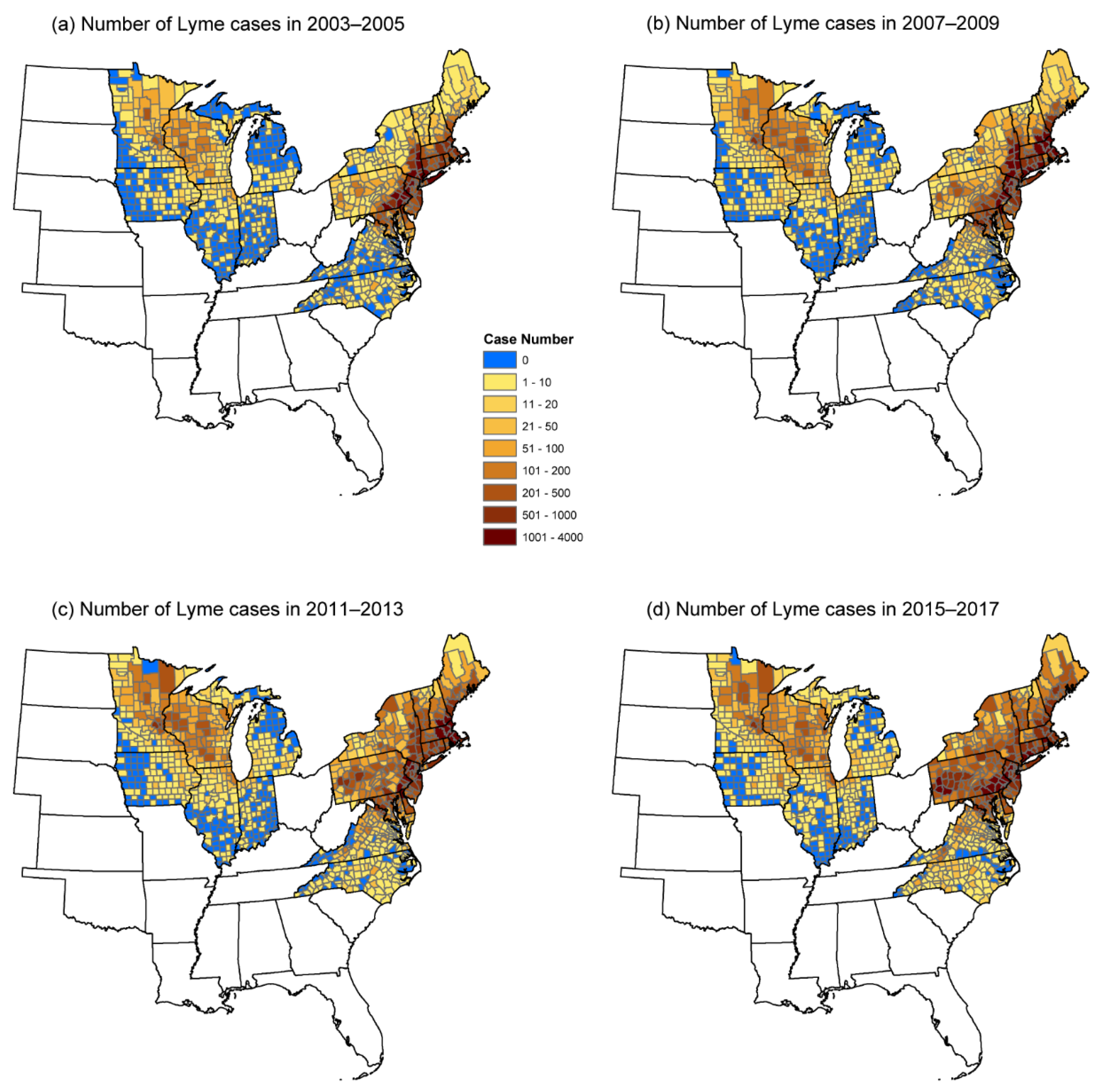
2.1. Lyme Disease Data

The study area included six states in the Upper Midwest and thirteen states in the Northeast (Figure 1), where the human Lyme cases were most frequently reported and accounted for almost 90% of all human cases in the USA (Centers for Disease Control and Prevention, CDC). It has been suggested that the disease in these two regions was mainly transmitted by the blacklegged tick, Ixodes scapularis [12,14]. According to a previous study [7], we here excluded those counties without the establishment of I. scapularis populations, as climatic and landscape factors play quite important roles in tick development and survival [26], and including the counties without tick might weaken the effects of these factors. In addition, as the spatial extent of Lyme disease is still spreading, we only included the counties where human cases were reported during 2003–2005 to avoid false absences (i.e., counties that reported human cases as zero before disease establishment).

As the life cycle of I. scapularis usually passes through 3 years [26], we consider comparing Lyme disease risk between two single years might not fully represent the true risk changes. Therefore, we collected the annual number of human Lyme cases and incidence for each county during two periods (i.e., 2003–2005 and 2015–2017) from the CDC (https://www.cdc.gov/ (accessed on 25 May 2020)). We then calculated the changes of human Lyme cases between two periods as:

$$\mathsf{\Delta }\mathrm{LymeRisk}=\log \left(\frac{\mathrm{total} \mathrm{number} \mathrm{of} \mathrm{human} \mathrm{cases} \mathrm{in} 2015–2017}{\mathrm{total} \mathrm{number} \mathrm{of} \mathrm{human} \mathrm{cases} \mathrm{in} 2003–2005}\right)$$

(1)

We also calculated the changes of Lyme incidence between the two periods in the same way.

2.2. Data of Predictors

As several previous studies suggested that climatic variables one year prior might be more predictive for Lyme disease risk [29], we here calculated, the seasonal mean temperature and precipitation (

Table 1. Description of climatic and landscape factors used in this study. X and Y relate to the season (for climatic variables) and land cover class (for landscape variables).

Predictors	Descriptions	Notes
Pre_X	Seasonal mean precipitation in previous year	X = (1. spring; 2. summer; 3. autumn; 4. Winter)
MeanT_X	Seasonal mean temperature in previous year
CA_Y	Total area of a land cover class	Y = (21–24,41–43)
ED_Y	Edge density of a land cover at the region

) during 2002–2004 and 2014–2016 for each county, based on the monthly values of these variables (with a grid cell of 0.5 × 0.5 degree) obtained from the Climate Research Unit datasets (CRUs) [30].

We collected the land-use cover maps for 2004 and 2016 from the National Land Cover Database (NLCD) [31]. Following previous studies [26], we here focused on seven land cover classes, four of which represent human-use area: developed-open space (class 21), developed space with low intensity (class 22), developed space with medium intensity (class 23), and developed space -high intensity (class 24). Another three classes related to forest habitat and represented, respectively, deciduous forest (class 41), evergreen forest (class 42), and mixed forest (class 43). We calculated the total area (CA) and the edge density (ED) for each land cover class and for each county (Table 1).

For each county, we calculated the changes of seasonal mean precipitation between the two periods (Pre_X) as:

$$\mathrm{Pre}\_\mathrm{X}=\frac{\mathrm{Pre}\_\mathrm{X}\left(2014–2016\right)-\mathrm{Pre}\_\mathrm{X}\left(2002–2004\right)}{\mathrm{Pre}\_\mathrm{X}\left(2002–2004\right)}$$

(2)

For the seasonal mean temperature, the changes of variables (MeanT_X) were calculated as the mean values of 2014–2016 minus those of 2002–2004. The changes of landscape variables between two periods were calculated in asimilar way with changes in precipitation.

2.3. Statistical Analyses

To investigate the effects of predictors on the changes in human Lyme risk between the two periods, we used general linear mixed models (LMM) with state as a random factor to control for the between-state variations. All predictor variables were scaled before performing LMMs.

We first fitted univariate models to test the effect of each predictor, and identified potential risk factors as the vairables with a p-value < 0.05 in univariate analyses. With these potential risk factors, we then conducted LASSO (Least absolute shrinkage and selection operator) regression, which was recently introduced into ecological studies [32], to construct multiple regression models. As a statistical regularization approach (LASSO regression), LASSO regression can not only deal with independent variables with multi-collinearity, but also improve models’ predictive accuracy by trading off between bias and variance in parameter estimates [33]. In LASSO regression, ten-fold cross selection (CV) is usually applied to find the turning regularization parameter, λ. However, disease data usually show spatial autocorrelation, which may bias the standard CV due to the dependency between training data and validation data [34]. We here applied a spatial CV [35] that can potentially reduce the overestimate of the real capacity of the spatial model to make reliable predictions in areas distant from the training set, and thus is important for evaluating the extrapolation capacity of a given model [35]. In this spatial CV, the data for the Upper Midwest and the Northeast, based on the State of the sample, were respectively divided into six-folds and thirteen-folds. Then, the spatial CV was performed to generate the optimal regularization parameter, λ, which then was used to construct the final LASSO model.

To test the robustness of our results from LASSO regression, we also performed traditional model averaging in multiple regression analyses. In these analyses, we first checked for the multi-collinearity by calculating the Pearson correlation coefficients (r) between the potential risk factors from the univariate analyses. For those variables that showed high multi-collinearity (with r > 0.7), we only used the variable with the smallest p-value in model averaging analyses [36]. We ranked the candidate models based on the changed AICc values [37]. We then considered the models within ΔAICc < 2 as competing models, and averaged the regression coefficient of each independent variable. In both univariate and multiple models, we control for the effect of area size by retaining the area of county (AREA) in the model, and the variable AREA was not penalized in LASSO. Statistical analyses were conducted in R 4.0.2 using the package lme4 [38], MuMIn [39] and glmnet [40].

3. Results

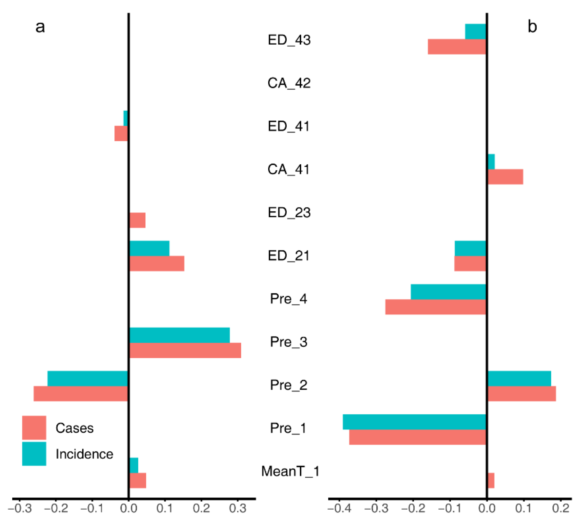
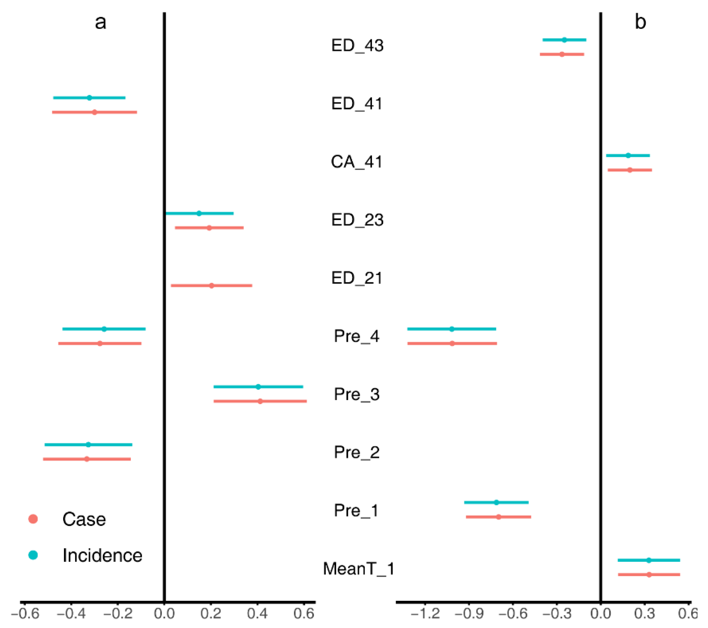
3.1. Univariate Regression Analyses

The univariate regression analyses for the changes of the human Lyme case numbers (

Table 2. Univariate regression results (standardized regression coefficient, b, and t) for the independent variables correlated with the changes of the number of human Lyme cases in the Upper Midwest (UM) and Northeast (NE).

Variables	Upper Midwest		Northeast
	b	t	b	t
Mean spring temperature	−0.35	−2.15 *	0.37	3.42 ***
Mean summer temperature	−0.12	−1.39	0.28	2.64 **
Mean autumn temperature	−0.21	−1.48	0.42	2.77 **
Mean winter temperature	0.07	0.75	0.13	0.86
Mean spring precipitation	−0.07	−0.59	−0.89	−8.36 ***
Mean summer precipitation	−0.30	−2.99 **	0.30	3.21 **
Mean autumn precipitation	0.47	4.76 ***	0.062	0.49
Mean winter precipitation	−0.22	−2.18 *	−1.18	−7.18 ***
Cover area of open space	0.29	3.71 ***	−0.08	−0.97
Edge density of open space	0.37	4.93 ***	−0.17	−2.22 *
Cover area of low-intensity space	0.25	3.21 **	−0.19	−2.45 *
Edge density of low-intensity space	0.27	3.54 ***	−0.18	−2.20 *
Cover area of medium-intensity space	0.18	2.18 *	−0.14	−1.62
Edge density of medium-intensity space	0.22	2.76 **	−0.13	−1.50
Cover area of high-intensity space	0.02	0.23	−0.04	−0.47
Edge density of high-intensity space	0.14	1.78	−0.06	−0.68
Cover area of deciduous forest	−0.20	−2.75 **	0.24	3.01 **
Edge density of deciduous forest	−0.38	−4.87 ***	0.01	0.14
Cover area of evergreen forest	0.04	0.49	−0.08	−1.05
Edge density of evergreen forest	−0.04	−0.49	−0.19	−2.45 *
Cover area of mixed forest	−0.18	−2.20 *	−0.11	−1.45
Edge density of mixed forest	−0.18	−2.25 *	−0.19	−2.45 *

* p < 0.05; ** p < 0.01, *** p < 0.001.

) showed similar results with the changes of human Lyme incidence (

Table 3. Univariate regression results (standardized regression coefficient, b, and t) for the independent variables correlated with the changes of human Lyme incidence in the Northeast (NE) and Upper Midwest (UM) United Sates.

Predictors	Upper Midwest		Northeast
	b	t	b	t
Mean spring temperature	−0.36	−2.22 *	0.39	3.63 ***
Mean summer temperature	−0.13	−1.53	0.30	2.83 **
Mean autumn temperature	−0.24	−1.67	0.45	2.93 **
Mean winter temperature	0.06	0.64	0.13	0.84
Mean spring precipitation	−0.08	−0.67	−0.92	−8.63 ***
Mean summer precipitation	−0.30	−2.94 **	0.32	3.32 **
Mean autumn precipitation	0.46	4.65 ***	0.08	0.61
Mean winter precipitation	−0.20	−2.07 *	−1.19	−7.22 ***
Cover area of open space	0.24	3.08 **	−0.12	−1.48
Edge density of open space	0.3	4.27 ***	−0.22	−2.76 **
Cover area of low-intensity space	0.19	2.49 *	−0.25	−3.17 **
Edge density of low-intensity space	0.22	2.81 **	−0.24	−2.93 **
Cover area of medium-intensity space	0.13	1.67	−0.20	−2.31 *
Edge density of medium-intensity space	0.18	2.21 *	−0.19	−2.21 *
Cover area of high-intensity space	−0.01	−0.12	−0.07	−0.89
Edge density of high-intensity space	0.10	1.31	−0.11	−1.26
Cover area of deciduous forest	−0.19	−2.59 **	0.25	3.02 **
Edge density of deciduous forest	−0.36	−4.61 ***	0.02	0.20
Cover area of evergreen forest	0.04	0.48	−0.07	−0.95
Edge density of evergreen forest	−0.04	−0.49	−0.18	−2.40 *
Cover area of mixed forest	−0.16	−2.04 *	−0.10	−1.33
Edge density of mixed forest	−0.17	−2.10 *	−0.17	−2.27 *

* p < 0.05; ** p < 0.01, *** p < 0.001.

). For climatic variables, change of mean spring temperature was negatively correlated with the changes of human Lyme risk in Upper Midwest of the United States, while showed a positive correlation with risk changes in the Northeast. In the Northeast, the change in disease risk was negatively associated with the changes in the mean spring and winter precipitation, while positively correlated with changes in the mean summer precipitation. Changes of disease risk in the Upper Midwest showed negative correlations with changes of mean precipitation in summer and winter, while positive correlation with precipitation in autumn.

For landscape factors, all indicators related to the human-use area (except for class 24) showed positive correlations with the changes of human Lyme risk in the Upper Midwest, while indicators related to developed-open space (class 21) and developed-low intensity space (class 22) showed negative correlations in the Northeast (Table 2 and Table 3). Deciduous forest variables showed negative associations with risk changes in the Upper Midwest, while positive correlations in the Northeast. In addition, risk change in the Upper Midwest was also negatively correlated with mixed forest, and risk change in the Northeast was also natively correlated with the edge densities of evergreen forest and mixed forest.

3.2. Multiple Regression Analyses

Generally, analyses on the change of human Lyme cases and incidence generated similar results for both LASSO regression (Figure 2) and model averaging (Figure 3). In both the Upper Midwest and the Northeast, the results only showed slight differences between LASSO regression and model averaging.

In the Upper Midwest (Figure 2a and Figure 3a), both the change of case number and incidence were negatively correlated with the changes of mean precipitation in summer (Pre_2), and the edge density of deciduous forests (ED_41); while positively correlated with the mean precipitation in autumn (Pre_3), the edge densities of open space (ED_21) and medium-intensity space (ED_23). LASSO regression (Figure 2a) also identified a negative correlation of the mean temperature in spring (MeanT_1).

In the Northeast (Figure 2b and Figure 3b), the results suggested that the risk change was positively associated with the change of mean temperature in spring (MeanT_1) and the cover area of deciduous forest (CA_41), while negatively correlated with the changes of mean precipitation in spring (Pre_1) and winter (Pre_4), and the edge density of mixed forest (ED_43). LASSO regression (Figure 2b) also identified a positive correlation of the mean precipitation in summer (Pre_2) and a negative correlation of edge density of open space (ED_21).

4. Discussion

In this study, we compared the spatial patterns of human Lyme risk in the Upper Midwest and Northeast of United States in two periods (2003–2005 and 2015–2017), and investigated the correlations between the changes of landscape/climatic factors and risk change. The results from univariate analyses suggested that climate and landscape variables generally showed different, even opposite, relationships with the changes in human Lyme risk in the Upper Midwest and Northeast. In addition, we used both model averaging and LASSO regression to construct the multiple regression models, which identified several but distinct risk factors for the two regions. In this discussion, we first discuss the effects of climatic and landscape factors on the change of human Lyme risk. Then, we compare the results from LASSO and model averaging and focus on the potential applications of LASSO approach and spatial cross validation. Finally, we acknowledge the limitation of this study and give suggestions for future research.

4.1. Effects of Climatic Factors

In our analyses, for precipitation variables, we found that change of mean summer precipitation was positively associated with the changes of human Lyme risk in the Northeast, which is consistent with a previous study showing that precipitation in early summer can favor tick survival in the Northeast [17]. However, the changes of mean spring and winter precipitation were negatively associated with changes of human risk changes in the Northeast. We consider this might be caused by the effects of precipitation on food availability for rodent species, many of which are competent hosts for Lyme disease. In the Northeast, the rainfall in winter and spring (86 mm and 101 mm respectively) were much higher than those in the Upper Midwest (24 mm and 77 mm respectively). Increasing winter and spring rainfall in this region might rot the food collected by rodents, reducing rodent abundance. For temperature variables, the results showed that changes in mean spring temperature were negatively associated with human risk changes in Upper Midwest, which is consistent with our expectation that ticks are vulnerable to high temperature. However, the positive effect of mean temperature we identified in the Northeast did not follow this expectation, but was consistent with a previous study suggesting that a high temperature at ground level is able to promote tick abundance [13]. In general, these results, consistent with several previous studies, showed that climatic variables could show considerably different effects on Lyme risk among different regions [5,29], and indicated that the changes of Lyme disease in these two regions might show different responses to the ongoing climate change.

4.2. Effects of Landscape Factors

For landscape factors, we found that, for each land cover type, the total area (CA) and the edge density (ED) are highly correlated, therefore, it is difficult to know which index had the true causal effect on the change of Lyme risk. Our results from the univariate regression analyses suggested that the landscape variables related to develop-space (class 21–23) generally had opposite effects on the risk change in the two regions, with positive associations in Upper Midwest and negative associations in the Northeast. We consider this result might be caused by the difference of development between the two regions. Generally, counties in the Upper Midwest were less developed than those in the Northeast, as suggested by lower percentage of develop-space area in the Upper Midwest (10.79% in 2003–2005) than that in the Northeast (21.61% in 2003–2005). Increasing develop-space area in the Upper Midwest may cause more edges between human residences and forests, leading to an increase in the contact rates between people and ticks. However, the negative effects of develop-space area identified in the Northeast were not consistent with previous studies, and needs more studies to explore the underlying mechanisms. For forest related factors, the deciduous forest has opposite correlations between the Upper Midwest and the Northeast. In the Upper Midwest, decreasing forests, particularly deciduous forest, might be correlated with more contacts of human to forests and ticks, thus can increase human Lyme disease risk. In addition, evergreen forests (class 42) and mixed forests (class 43) generally had negative effects on Lyme disease risk, which was consistent to several previous studies assuming that these forests might be poor environments for ticks regarding to temperature and precipitation as they were generally located in mountainous areas [26]. In general, the climatic and landscape factors showed divergent effects on the changes in human Lyme risk in the two regions. We consider this result might attribute to the differences in tick and pathogen dispersal and distributions between the regions, which can be contributed by the differences in the dominant reservoir host species [3].

4.3. LASSO and Model Averaging

Landscape metrics are notorious numerous, and some of them are correlated with each other, including these metrics, particularly the metrics without explicit hypotheses, may lead to a high chance of detecting spurious correlations and over-fit of the model. Moreover, as disease risk data usually show spatial autocorrelation (e.g., cluster geographically), random partition of the data into training and validation sets can lead to over-fit of the spatial model and overestimate the capacity of the model to make reliable predictions in regions far away from the training set [35]. We thus here applied a LASSO approach integrated with spatial cross validation (spatial CV), together with traditional model averaging approach, to construct multiple regression models. The results from these two different approaches were quite similar. We consider this might be caused by the little spatial-autocorrelation of the change in Lyme risk, as suggested by low Moran’s I indices (0.131 and 0.134 for case number change and incidence change in the Upper Midwest, 0.056 and 0.051 in the Northeast).

With increasing high-resolution land cover data and advances in remote sensing techniques, scientists have been showing more and more interest in exploring the roles of landscape factors on pathogen transmission [41,42]. We consider our approach could be applied in the future studies which try to map the risk of infectious diseases using landscape metrics.

4.4. Limitations

We must admit that the Lyme case number obtained from CDC might be an underestimate of actual human cases. Particularly, different states may apply different approaches to gather case data. Including state as a random effect in our analyses was able to control for, to some extent, the differences in surveillance way among states. In addition, we admit that other socioeconomic (e.g., human behavior) or biotic factors (e.g., tick density, host community composition, etc.) could be also important in determining human Lyme disease risk. However, due to the lack of landscape-scale data of these factors, we could not control for these factors. Finally, this study focus on the correlations between Lyme risk changes and predictors, and may not disclose the causality underlying the detected relationships, we thus suggest future studies could explore the underlying mechanisms with more field data, such as the fluctuation of rodent density or tick density. Despite of the limitations of our analyses, this study is the first study, to our knowledge, trying to investigate and compare the drivers of spatial patterns in Lyme risk change in two “highly endemic” regions in the United States. In addition, we consider the findings here in Lyme disease may also be applied in other I. scapularis-transmitted diseases, such as Anaplasmosis and Babesiosis which are also most frequently reported in the Upper Midwest and the Northeast.

5. Conclusions

In this study, we compared the spatial patterns of human Lyme disease in the Upper Midwest and Northeast of United States in two periods (2003–2005 and 2015–2017), and investigate the correlations of the changes in climatic and landscape variables with these patterns. Our analyses demonstrated that variables related to climate and landscape factors generally had different, even opposite, effects on the changes of human Lyme disease in the two regions. Besides, even in the same region, the correlations of changes of precipitation vary among different seasons. Changes of human-use area show opposite effects on changes of human Lyme disease in these two regions. Generally, our results indicated that the changes of human Lyme disease in the two regions may show different responses to the ongoing changes in climate and land use, which might be beneficial to the future prediction of Lyme disease. As this is a correlation analysis which cannot disclose the causality for the detected relationships, we suggest future studies could explore the ecological mechanisms underlying the correlations we found, by collecting detailed field data such as rodent and tick density.

References

1. Turney, S.; Gonzalez, A.; Millien, V. The negative relationship between mammal host diversity and Lyme disease incidence strengthens through time. Ecology 2014, 95, 3244–3250. [Google Scholar] [CrossRef]
2. Wang, Y.X.; Matson, K.D.; Xu, Y.; Prins, H.H.; Huang, Z.Y.; de Boer, W.F. Forest connectivity, host assemblage characteristics of local and neighboring counties, and temperature jointly shape the spatial expansion of lyme disease in United States. Remote. Sens. 2019, 11, 2354. [Google Scholar] [CrossRef] [Green Version]
3. Gardner, A.M.; Pawlikowski, N.C.; Hamer, S.A.; Hickling, G.J.; Miller, J.R.; Schotthoefer, A.M.; Tsao, J.I.; Allan, B.F. Landscape features predict the current and forecast the future geographic spread of Lyme disease. Proc. R. Soc. B 2020, 287, 20202278. [Google Scholar] [CrossRef] [PubMed]
4. Dumic, I.; Severnini, E. “Ticking bomb”: The impact of climate change on the incidence of Lyme disease. Can. J. Infect. Dis. Med. 2018, 2018, 5719081. [Google Scholar] [CrossRef] [PubMed] [Green Version]
5. Dong, Y.; Huang, Z.; Zhang, Y.; Wang, Y.X.; La, Y. Comparing the Climatic and Landscape Risk Factors for Lyme Disease Cases in the Upper Midwest and Northeast United States. Int. J. Environ. Res. Public Health 2020, 17, 1548. [Google Scholar] [CrossRef] [PubMed] [Green Version]
6. Hofmeester, T.R.; Jansen, P.A.; Wijnen, H.J.; Coipan, E.C.; Fonville, M.; Prins, H.H.; Sprong, H.; van Wieren, S.E. Cascading effects of predator activity on tick-borne disease risk. Proc. R. Soc. B 2017, 284, 20170453. [Google Scholar] [CrossRef] [Green Version]
7. Eisen, R.J.; Piesman, J.; Zielinski-Gutierrez, E.; Eisen, L. What do we need to know about disease ecology to prevent Lyme disease in the northeastern United States? J. Med. Entomol. 2012, 49, 11–22. [Google Scholar] [CrossRef]
8. Kilpatrick, A.M.; Dobson, A.D.; Levi, T.; Salkeld, D.J.; Swei, A.; Ginsberg, H.S.; Kjemtrup, A.; Padgett, K.A.; Jensen, P.M.; Fish, D. Lyme disease ecology in a changing world: Consensus, uncertainty and critical gaps for improving control. Philos. Trans. R. Soc. B Biol. Sci. 2017, 372, 20160117. [Google Scholar] [CrossRef]
9. Ostfeld, R.S.; Canham, C.D.; Oggenfuss, K.; Winchcombe, R.J.; Keesing, F. Climate, Deer, Rodents, and Acorns as Determinants of Variation in Lyme-Disease Risk. PLoS Biol. 2006, 4, e145. [Google Scholar] [CrossRef]
10. Lindgren, E.; Tälleklint, L.; Polfeldt, T. Impact of climatic change on the northern latitude limit and population density of the disease-transmitting European tick Ixodes ricinus. Environ. Health Perspect. 2000, 108, 119–123. [Google Scholar] [CrossRef]
11. McPherson, M.; García-García, A.; Cuesta-Valero, F.J.; Beltrami, H.; Hansen-Ketchum, P.; MacDougall, D.; Ogden, N.H. Expansion of the Lyme disease vector Ixodes scapularis in Canada inferred from CMIP5 climate projections. Environ. Health Perspect. 2017, 125, 057008. [Google Scholar] [CrossRef] [PubMed] [Green Version]
12. Eisen, R.J.; Eisen, L.; Ogden, N.H.; Beard, C.B. Linkages of weather and climate with Ixodes scapularis and Ixodes pacificus (Acari: Ixodidae), enzootic transmission of Borrelia burgdorferi, and Lyme disease in North America. J. Med. Entomol. 2016, 53, 250–261. [Google Scholar] [CrossRef] [PubMed] [Green Version]
13. Werden, L.; Barker, I.K.; Bowman, J.; Gonzales, E.K.; Leighton, P.A.; Lindsay, L.R.; Jardine, C.M. Geography, deer, and host biodiversity shape the pattern of Lyme disease emergence in the Thousand Islands archipelago of Ontario, Canada. PLoS ONE 2014, 9, e85640. [Google Scholar] [CrossRef] [PubMed] [Green Version]
14. Ostfeld, R.S.; Brunner, J.L. Climate change and Ixodes tick-borne diseases of humans. Philos. Trans. R. Soc. B Biol. Sci. 2015, 370, 20140051. [Google Scholar] [CrossRef] [PubMed] [Green Version]
15. Clark, D.D. Lower temperature limits for activity of several Ixodid ticks (Acari: Ixodidae): Effects of body size and rate of temperature change. J. Med. Entomol. 1995, 4, 449–452. [Google Scholar] [CrossRef]
16. Ogden, N.H.; Lindsay, L.R.; Beauchamp, G.; Charron, D.; Maarouf, A.; O’Callaghan, C.J.; Waltner-Toews, D.; Barker, I.K. Investigation of Relationships Between Temperature and Developmental Rates of Tick Ixodes scapularis (Acari: Ixodidae) in the Laboratory and Field. J. Med. Entomol. 2004, 41, 622–633. [Google Scholar] [CrossRef] [Green Version]
17. McCabe, G.J.; Bunnell, J.E. Precipitation and the occurrence of Lyme disease in the northeastern United States. Vector. Borne. Zoonotic. Dis. 2004, 4, 143–148. [Google Scholar] [CrossRef]
18. Ballard, K.; Bone, C. Exploring spatially varying relationships between Lyme disease and land cover with geographically weighted regression. Appl. Geogr. 2021, 127, 102383. [Google Scholar] [CrossRef]
19. Diuk-Wasser, M.A.; VanAcker, M.C.; Fernandez, M.P. Impact of Land Use Changes and Habitat Fragmentation on the Eco-epidemiology of Tick-Borne Diseases. J. Med. Entomol. 2020, 58, 1546–1564. [Google Scholar] [CrossRef]
20. Killilea, M.E.; Swei, A.; Lane, R.S.; Briggs, C.J.; Ostfeld, R.S. Spatial dynamics of lyme disease: A review. Ecohealth 2008, 5, 167–195. [Google Scholar] [CrossRef] [Green Version]
21. Wood, C.L.; Lafferty, K.D. Biodiversity and disease: A synthesis of ecological perspectives on Lyme disease transmission. Trends Ecol. Evol. 2013, 28, 239–247. [Google Scholar] [CrossRef] [PubMed]
22. Bertrand, M.R.; Wilson, M.L. Microclimate-dependent survival of unfed adult Ixodes scapularis (Acari: Ixodidae) in nature: Life cycle and study design implications. J. Med. Entomol. 1996, 33, 619–627. [Google Scholar] [CrossRef] [PubMed]
23. Schulze, T.L.; Jordan, R.A.; Hung, R.W. Suppression of subadult Ixodes scapularis (Acari: Ixodidae) following removal of leaf litter. J. Med. Entomol. 1995, 32, 730–733. [Google Scholar] [CrossRef] [PubMed]
24. Brownstein, J.S.; Skelly, D.K.; Holford, T.R.; Fish, D. Forest fragmentation predicts local scale heterogeneity of Lyme disease risk. Oecologia 2005, 146, 469–475. [Google Scholar] [CrossRef] [PubMed]
25. Horobik, V.; Keesing, F.; Ostfeld, R.S. Abundance and Borrelia burgdorferi-infection prevalence of nymphal Ixodes scapularis ticks along forest–field edges. EcoHealth 2006, 3, 262–268. [Google Scholar] [CrossRef] [Green Version]
26. Tran, P.M.; Waller, L. Effects of landscape fragmentation and climate on Lyme disease incidence in the northeastern United States. Ecohealth 2013, 10, 394–404. [Google Scholar] [CrossRef] [PubMed]
27. Li, S.; Hartemink, N.; Speybroeck, N.; Vanwambeke, S.O. Consequences of landscape fragmentation on Lyme disease risk: A cellular automata approach. PLoS ONE 2012, 7, e39612. [Google Scholar] [CrossRef] [Green Version]
28. Millins, C.; Dickinson, E.R.; Isakovic, P.; Gilbert, L.; Wojciechowska, A.; Paterson, V.; Tao, F.; Jahn, M.; Kilbride, E.; Birtles, R.; et al. Landscape structure affects the prevalence and distribution of a tick-borne zoonotic pathogen. Parasit Vector 2018, 11, 621. [Google Scholar] [CrossRef]
29. Schauber, E.M.; Ostfeld, R.S.; Evans, J.; Andrew, S. What is the best predictor of annual Lyme disease incidence: Weather, mice, or acorns? Ecol. Appl. 2005, 15, 575–586. [Google Scholar] [CrossRef]
30. Harris, I.; Jones, P.D.; Osborn, T.J.; Lister, D.H. Updated high-resolution grids of monthly climatic observations—The CRU TS3. 10 Dataset. Int. J. Climatol. 2014, 34, 623–642. [Google Scholar] [CrossRef] [Green Version]
31. Wickham, J.; Homer, C.; Vogelmann, J.; McKerrow, A.; Mueller, R.; Herold, N.; Coulston, J. The multi-resolution land characteristics (MRLC) consortium—20 years of development and integration of USA national land cover data. Remote. Sens. 2014, 6, 7424–7441. [Google Scholar] [CrossRef] [Green Version]
32. Tredennick, A.T.; Hooker, G.; Ellner, S.P.; Adler, P.B. A practical guide to selecting models for exploration, inference, and prediction in ecology. Ecology 2021, 102, e03336. [Google Scholar] [CrossRef]
33. Hastie, T.; Tibshirani, R.; Friedman, J. The Elements of Statistical Learning: Data Mining, Inference, and Prediction; Springer: New York, NY, USA, 2009. [Google Scholar]
34. Randin, C.F.; Dirnböck, T.; Dullinger, S.; Zimmermann, N.E.; Zappa, M.; Guisan, A. Are niche-based species distribution models transferable in space? J. Biogeogr. 2006, 33, 1689–1703. [Google Scholar] [CrossRef]
35. Dhingra, M.S.; Artois, J.; Robinson, T.P.; Linard, C.; Chaiban, C.; Xenarios, I.; Engler, R.; Liechti, R.; Kuznetsov, D.; Xiao, X. Global mapping of highly pathogenic avian influenza H5N1 and H5Nx clade 2.3. 4.4 viruses with spatial cross-validation. eLife 2016, 5, e19571. [Google Scholar] [CrossRef] [PubMed]
36. Zuur, A.F.; Ieno, E.N.; Elphick, C.S. A protocol for data exploration to avoid common statistical problems. Methods. Ecol. Evol. 2010, 1, 3–14. [Google Scholar] [CrossRef]
37. Burnham, K.P.; Anderson, D.R.; Huyvaert, K.P. AIC model selection and multimodel inference in behavioral ecology: Some background, observations, and comparisons. Behav. Ecol. Sociobiol. 2011, 65, 23–35. [Google Scholar] [CrossRef]
38. Bates, D.; Sarkar, D.; Bates, M.D.; Matrix, L. The lme4 package. R Package Version 2007, 2, 74. [Google Scholar]
39. Barton, K. MuMIn: Multi-Model Inference. 2009. Available online: http://r-forge.r-project.org/projects/mumin/ (accessed on 23 April 2022).
40. Hastie, T.; Qian, J.; Tay, K. An Introduction to Glmnet. CRAN R Repositary. 2021. Available online: https://cloud.r-project.org/web/packages/glmnet/vignettes/glmnet.pdf (accessed on 23 April 2022).
41. Ostfeld, R.S.; Glass, G.E.; Keesing, F. Spatial epidemiology: An emerging (or re-emerging) discipline. Trends Ecol. Evol. 2005, 20, 328–336. [Google Scholar] [CrossRef]
42. Estrada-Peña, A.; Ostfeld, R.S.; Peterson, A.T.; Poulin, R.; de la Fuente, J. Effects of environmental change on zoonotic disease risk: An ecological primer. Trends Parasitol. 2014, 30, 205–214. [Google Scholar] [CrossRef]
Figure 1. Spatial pattern of the number of human Lyme cases in 2003–2005 (a), 2007–2009 (b), 2011–2013 (c), and 2015–2017 (b).
Sustainability 14 05802 g001
Figure 2. The coefficients for LASSO regression models for the Upper Midwest (a) and the Northeast (b). MeanT_1, changes of mean spring temperature; Pre_X, changes of seasonal mean precipitation (X = [1, spring; 2, summer; 3, autumn; 4, winter]); CA_Y, total area of a land cover class; ED_Y, edge density of a land cover class (Y = [21, developed-open space; 23, developed-medium intensity space; 41, deciduous forest; 42, evergreen forest; 43, mixed forest]).
Sustainability 14 05802 g002
Figure 3. The regression coefficients and their 95% CI of model averaging for the Upper Midwest (a) and the Northeast (b). MeanT_1, changes of mean spring temperature; Pre_X, changes of seasonal mean precipitation (X = [1, spring; 2, summer; 3, autumn; 4, winter]); CA_41, total area of deciduous forests; ED_Y, edge density of a land cover class (Y = [21, developed-open space; 23, developed-medium intensity space; 41, deciduous forests; 43, mixed forests]).
Sustainability 14 05802 g003