Using Bidirectional Long-Term Memory Neural Network for Trajectory Prediction of Large Inner Wheel Routes

Abstract

When a large car turns at an intersection, it often leads to tragedy because the driver does not pay attention to the incoming car or the dead corner of the line of sight of the car body. On the market, the wheel difference warning system used in large cars generally adds sensors or lenses to confirm whether there are incoming vehicles in the dead corner of the line of sight. However, the accident rate of large vehicles has not been reduced due to the installation of a vision subsidy system. The main reason is that motorcycle and bicycle drivers often neglect to pay attention to the inner wheel difference formed when large vehicles turn, resulting in accidents with large vehicles at intersections. This paper proposes a bidirectional long-term memory neural network for the prediction of the inner wheel path trajectory of large cars, mainly from the perspective of motorcycle riders, through the combination of YOLOv4 and the stacked Bi-LSTM model used in this study to analyze the motion of large cars and predict the inner wheel path trajectory. In this study, the turning trajectory of large vehicles at the intersection is predicted by using an object detection algorithm and cyclic neural network model. Finally, the experiment shows that this study uses the stacked Bi-LSTM trajectory prediction model to predict the next second trajectory with one second trajectory data, and the prediction accuracy is 87.77%; it has an accuracy of 75.75% when predicting the trajectory data of two seconds. In terms of prediction error, the system has a better prediction error than LSTM and Bi-LSTM models.

1. Introduction

Traffic accidents worldwide cause more than 1.35 million deaths and 20–50 million serious injuries every year [1]. Therefore, many studies are being carried out on how to prevent traffic accidents and reduce damage. This kind of research is mainly to deduce the accident-prone sections by analyzing the historical data based on the road, to minimize the loss after the accident [2,3,4]. With the progress of traffic monitoring and image recognition, vehicle trajectory data is gradually used in recent research. Trajectory data includes vehicle dynamic information, such as vehicle position, speed, acceleration, etc. [5,6]. According to these data, various alternative safety measures based on traffic accidents are analyzed and predicted to reduce the occurrence and damage of traffic accidents.

In Taiwan, mass transportation has brought many mobile conveniences to our lives. All counties and cities have convenient mass transportation. In addition to fast moving modes such as MRT, trains, etc., the mass transportation in the city is mainly bus. The bus set up in each county and city is very convenient and has the characteristics of short time intervals and clear purpose, allowing us to choose a way of moving.

Not every city has a well-developed mass transportation network. Most people in other regions still use cars and locomotives as the main vehicle, which also leads to Taiwan’s top car density in the world. Combined with factors such as small roads in Taiwan, route planning, serious mixed traffic flow, passers-by habits and other factors, resulting in traffic accidents more serious than advanced countries, large cars at some junctions or traffic lights start in large numbers. The traffic accident causes a lot of regret.

Cars are roughly classified by use for buses, vans and special vehicles. The classification is divided into large and small cars. Small trucks, trucks, minibuses and buses are usually built according to the use of different forms, such as box trucks carrying solid bulk cargo, tank trucks carrying liquid class, etc.; different forms of vehicle body cause vision dead angle, roughly the height of the driver’s eye and the body structure of the car. Despite the large car body height, the driver’s eye position can see far, other than its front view dead angle and rear vision. The range of dead corners is much larger than small cars. While the installation of auxiliary devices such as mirrors, reversing radar, monitors and sensors helps improve the driver’s field of view, there is still a range of reflections or no shots.

The road killer of a large car internal wheel difference creates visual dead horns, claiming many lives every year. Figure 1 shows the number of large car accidents in the past five years. Large trucks are about twice the number of buses. Since many industries rely on large cargo vehicles, if sufficient safety warning devices are available, they will effectively reduce the accidents that occur. As a result, the Ministry of Transport has particularly promoted the law amendment, and in 2020, trucks and buses will need to install a driving vision assistance system and include regular inspection projects. However, there are still many driving reactions, and eyes on the screen of the auxiliary system will be distracted.

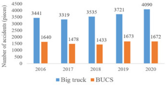
Figure 1. Statistics on the number of large car traffic accidents [7].

The market is widely used in the large vehicle wheel difference warning system to install sensors or lenses in large car bodies to confirm if there is a dead end of sight. However, the accident rate of large cars has not been reduced because of the installation of the field of view subsidy system, and locomotive and bicycle drivers still do not pay attention to the driving safety distance, and negligently pay attention to the inner wheel difference when the large car turns, causing accidents with large cars at the intersection.

In recent years, many trajectory prediction models based on the deep neural network (DNN) have been proposed [8,9,10]; the recurrent neural network (RNN), represented by long short-term memory (LSTM), has natural advantages in processing time series, which promotes the research on vehicle trajectory prediction [11,12]. Car trajectory prediction mainly uses the trajectory data of different vehicles to predict the next position or continuous trajectory to which the vehicle will move. Most of the existing studies collect and predict the trajectory based on aerial photos or camera images, but less so from the perspective of motorcycles or cyclists.

In today’s camera imaging resolution improvement, image recognition, data analysis and various intelligent technologies are developing rapidly, exploring the foresight and practicality of each technology. Through intelligent image recognition and deep learning, our main purpose is to detect large cars by using the system on the locomotive, from the perspective of the rider of the locomotive, through combining deep learning and machine vision. The action and analysis of movement trajectory during turn analyzes the inner wheel trajectory of a large car turn and predicts its future trajectory, alerting the locomotive rider to dangerous areas and reducing the chance of accidents with large cars.

This paper predicts the trajectory of the inner wheel during the turning of large cars using deep learning and the first training of image recognition models and cyclic neural network models from the perspective of locomotive or cyclists at the intersection. Using AI learning and image recognition technology, neural network models can analyze known and unknown objects. Using today’s proven algorithms to quickly dig and analyze the information and characteristics of various objects, so that computer devices can be like humans, and analyzing and predicting objects by object texture, size and direction of motion, demonstrates their ability to learn and manipulate even unknown things.

This paper focuses on intelligent image recognition, the circulating neural network and the trajectory prediction system, analyzing the turning trajectory of large cars and predicting their future position and movement. The so-called “intelligent image recognition”, in the early stages of development, means converting the reality information observed by humans into digital information that computers can understand, and allows the machine to continue to learn to have the same ability to recognize as human beings. Ultimately, it can be applied to more intelligent computing and recognition systems, and eventually to more intelligent computing and recognition systems. While a “circulating neural network” improves the traditional neural network and can only look at the current information problem alone, the information in the network cycle, as well as having memory, according to past memory and experience, can make predictions and judgments. The final “trajectory prediction” is to determine the direction and trajectory of the object in the future by giving the target object’s movement trajectory data over a period of time, by analyzing the information in the data.

This paper is divided into five sections. The first section presents the background, motivation and purpose of this paper. The second section is a study on the literature, including the development of image detection and trajectory prediction, which summarizes the knowledge of relevant research, and serves as the basis for the theoretical development of this paper. The third section is the system architecture of this paper. This paper provides an overview of the system architecture in a schematic diagram, followed by a detailed description of the image detection and circulating neural networks used by the system. The fourth section introduces the simulation environment, deep learning training process, and then analyzes and compares the experimental data results. This paper is summarized in Section 5, which includes its contributions, recommendations and improvements in future research directions.

2. Related Work

2.1. Object Detection

Image classification and object detection have become two of the most exciting fields in computer vision and artificial intelligence. Convolutional neural network (CNN) architecture develops rapidly with the explosive growth of computer computing speed. Today’s computer technology can perform well in certain specific situations (e.g., face recognition, handwritten digital recognition, image classification). In the process of neural network development, many of the already collated data sets are also increasingly available to developers on the web, which also allows neural networks to develop faster.

2.1.1. MobileNet

Ref. [13] Mobilenet is a convolutional neural network model architecture proposed by the Google team in 2017, due to the general architecture of some mobile or embedded devices in the hardware device Based on the problem of large convulvative neural network models, the overly large model leads to computational disadvantage for use on lower order hardware devices. Google proposes a new computational convouvator network method called Depthwise convolution and Pointwise convolution.

Generally, in a large network model, most of the calculations are in convolutional neural networks, with W, H and N as the width, height and dimensions of the input data, multiplied by N_k input dimensions to k × k convolutional core; the final output of the width, height and dimensions W_out, H_out and N_k, and the total calculation amount is shown in Equation (1).

$$\mathrm{calculation} \mathrm{amount}=\mathrm{W}·\mathrm{H}·\mathrm{N}·k^2·N_k$$

(1)

The concept proposed by MobileNet is to reduce the amount of calculations without affecting the structure of the final output result, and split it into two parts, namely Depthwise convolution with Pointwise convolution. The Depthwise convolution calculation first establishes individual k × k convolution cores for each dimension on the input, and then each dimension for the corresponding convolution core are calculated separately. The general convolution calculation is generally calculated by putting all the dimensions together, but here it is conducted independently, as shown in Equation (2).

$$\mathrm{calculation} \mathrm{amount}=\mathrm{W}·\mathrm{H}·\mathrm{N}·k^2$$

(2)

The Pointwise convolution calculation is the N dimension data of the H’ × W’ size resulting from the Depthwise convolution calculation, and then for the N_k 1 × 1 × N convolution, the calculated amount is shown in Equation (3); the combined result will be the same as the general convolution calculation output.

$$\mathrm{calculation} \mathrm{amount}=\mathrm{W}·\mathrm{H}·\mathrm{N}·N_k$$

(3)

By Equations (1)–(3) with the general convolution total calculation amount, the molecule with the total amount proposed by Mobilenet can be collated to obtain the formula, and the calculation in Equation (4) can be observed. The volume is increased by 1/N + 1/k² times, which means that the larger the convolution core size with the more numbers can save more calculations, such as 512 × 512 × 50 input data, and there are 10. With a convolutional core size of 5 × 5, the Depthwise separable convolution has only a 1/10 + 1/25 = 0.14 computation of general convolution.

$$\frac{\mathrm{W}·\mathrm{H}·\mathrm{N}·k^2+\mathrm{W}·\mathrm{H}·\mathrm{N}·N_k}{\mathrm{W}·\mathrm{H}·\mathrm{N}·k^2·N_k}=\frac{1}{N_k}+\frac{1}{k^2}$$

(4)

In 2018 [14], the version of MobilenetV2 adds linear bottlenecks to the depth separable convolution of MobileNetV1 (linear bottlenecks) and Inverted Residuals (Inverted Residuals), and reduced the amount of computations and increased accuracy from 89.9% to 91%. MobilenetV2 not only reduces more computations, but also improves the accuracy of recognition.

2.1.2. You Only Look Once (YOLO)

Ref. [15] YOLOv1 was proposed in 2015; its core concept compared to R-CNN is to put forward the region and then judge and look at the only area; thus, the scope is relatively small, with the Background patch being easy to see as an object. However, YOLOv1 looks at the entire picture at the time of training and detection, and directly at the output layer using the regression algorithm to calculate the position and category of b-box; thus, the background error detection rate (background error) is half the Fast R-CNN.

YOLOv1 has very small objects that are close to each other, because a grid cell only predicts two b-boxes and ends up with only one category. In addition, because only two b-boxes are used, the detection effect is poor for uncommon objects in length and width.

The changes are shown in Table 1 [16]; YOLOv2 is built on top of YOLOv1 and proposed in 2016. YOLOv2 has better accuracy and faster detection speed and can detect up to 9000 kinds of objects. [17] YOLOv3 has not made a special innovation; in order to take detection accuracy to the next level, the new network base is Darknet-53, compared to the previous Darknet-19 Deeper layers, and the ResNet structure commonly used in the general neural network deepening is used to solve the gradient problem.

Table 1. Table of improvement methods for YOLOV2 model.

Directions for Improvement	Method
More accurate for detection	Batch normalization	High resolution classifier	Convolutional with anchor boxes	Dimension clusters
	Direct location prediction	Fine-grained features	Multi-scale training
Faster for detection	Darknet-19	Training for classifier	Training for detection

To improve the detection of small objects, feature pyramid networks ([18] FPN) are used, and feature layers are changed from single layers to multiple layers. The number of layers of the type has dimensions of 13 × 13, 26 × 26 and 52 × 52, and the number of b-boxes each layer 5 into 3, thus it is a total output of 3 × 3. Using the FPN architecture compares the b-box of the next layer to the previous layer, and selects a better position to merge semantic features, making detection of small objects very good.

Ref. [19] In April 2020 by Alexey Bochkovskiy et al., the YOLOv3 structure is divided into input, backbone, neck and prediction. The original input uses the Mosaic data amplification method to enrich the data set and improve the performance of the model for small object detection, arrange and zoom.

The name is changed to CSPDarknet53 in the Backbone side and the former Darknet53 to CSPNet (Cross Stage Partial) Network) as a structure, which is composed of CBM + CSPX; CBM is a combination of Conv2d + BN and Mish activation function. The difference from YOLOv3 is that the BN changed the Cross mini-Batch Normalization (CmBN), which can be applied to smaller batch sizes. In addition, in order to avoid overfitting, the dropout of YOLOv3 is changed to Dropblock, ignoring the whole area neuron at a time than the original dropout is more advantageous. The dropout will randomly delete multiple neurons, but when the network layer increases, the model can still predict from the deleted nearby neurons, losing random dropout intent.

The Neck structure combines the Path Aggregation Network (PANet) architecture with the Spatial in addition to the original FPN architecture Pyramid Pooling (SPP) structure, in addition to improving the detection effect of small size targets; PANet splits the underlying features of the network and enhanced upwards to make the upper layer. The structure can also have the underlying edge shape feature, thus improving the detection of large objects, and SPP can effectively align the anchor box with the position of the feature map and increase accuracy. Table 2 calculates the main differences between YOLOv3 and YOLOv4.

Table 2. Comparison of YOLOv3 and YOLOv4.

Architecture and Methodical	YOLOv3	YOLOv4	Improvement Advantages
Prediction (Head)	YOLO	YOLO
Data augmentation	Pixel-wise adjustments	Mosaic	Stitching 4 images into one can reduce mini-batches by 4 times and improve detection of small objects
Backbone	Darknet53	CSPDarknet53	Reduces the number of parameters, reduces the amount of operation and improves accuracy
Normalization	Batch normalization (BN)	Cross mini-Batch Normalization (CmBN)	Can be better suited for smaller batch size settings
Neck	FPN	FPN + PAN + SPP	Combining local features and global feature messages to obtain rich semantic feature plots
Regularization	Dropout	Dropblock	Avoiding disturbance between neighboring neurons
Activations	Leaky-ReLU	Leaky-ReLU andMish	Mish function makes gradient smoother and stable

2.1.3. Faster Region-Based CNN, Faster R-CNN

Ref. [20] Faster R-CNN is an improved version of [21] R-CNN and [22] Fast R-CNN. Both models of R-CNN or Fast R-CNN basically need a Selective Search before calculating the feature map to produce a number of possible regions (Region Proposals). This part of the algorithm is the result of a loop method; thus, the calculation here is slow. A faster R-CNN was presented in 2016, and is a faster R-CNN model than the first two.

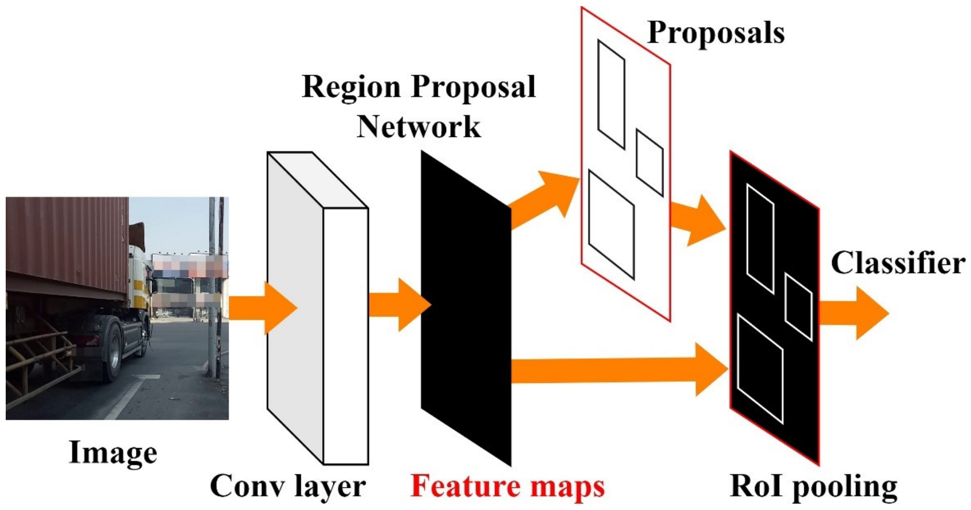
Faster R-CNN is intuitive; instead of producing Region Proposals from a slow Selective Search, instead the image is computed directly after the CNN feature map, which then passes through the Region Proposal Network layer (Region Proposal Network, RPN). Several Region Proposals are obtained and the final result is obtained from the RoIPooling layer such as Fast RCNN, as shown in Figure 2.

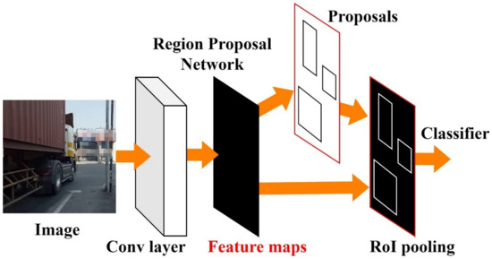
Figure 2. Ref. [8] Faster R-CNN model architecture diagram.

The feature map output of CNN contains the probability of b-box and the b-box objects. Because RPN is a convolutional network, RPN can enter the previous output of CNN. In RPN it is calculated by the sliding window and its center point is called the anchor point. The k different size set in the model parameters before training the Scale box calculates the probability score (score) that the object may contain in anchor point, taking the highest as the box. Finally, by RPN calculation one can obtain some b-boxes, although these are not necessarily accurate; however, after the last RoIPooling, one can quickly classify each box and find the most accurate b-box.

2.1.4. Single Shot Multi-Box Detector

In 2015, the Google team proposed a neural network detection model for rapid detection, called [23] SSD, which does not come from Faster R-CNN High accuracy. However, it has a relatively fast test execution time, although it is not as fast as YOLO; however, there is a relatively high detection accuracy.

2.2. Basic LSTM Encoder–Decoder Trajectory Deposit Method

In recent years, with the rise of autonomous cars, there are many ways to predict future trajectories of objects in terms of determining how objects move and accurately predicting the future trajectory of moving targets. This paper will introduce trajectory prediction methods, including inverse reinforcement learning, deep learning-based trajectory prediction and LSTM-based Encoder–Decoder trajectory prediction Methods.

Kitani et al. [24] use state machines to predict location. First of all, they cut the roads to be predicted into many small grids, each with its own location in the space, calling it states, and using the general Markov model of the decision process to optimize the problem. Thus, they use inverse reinforcement learning, hoping to learn the reward function from past trajectory messages and state appearance messages. An algorithm that makes important assumptions about the reward function, as shown in Equation (5), is a reward function that converts the observed state characteristic f(s) into a single cost value. θ is a vector to learn weights, and it will learn how much physics scene features affect a person’s behavior. The cost function parameter, θ, is optimized by maximizing the entropy of a conditional distribution. As shown in Equation (6), the eigenvector $f\prime \left(s_t\right)$ includes a tracking observation feature of state s_t and past actions u. Z(θ) is a normalized function.

$$r\left(s;\theta \right)={\theta }^{T}f\left(s\right)$$

(5)

$$r\left(s|u;\theta \right)=\frac{e\left\{{{\displaystyle \sum }}_t{\theta }^{T}f\prime \left(s_t\right)\right\}}{Z\left(\theta \right)}$$

(6)

Deep learning has been a popular and leading visual representation technology in recent years. It is also used for many forecasting tasks, such as video prediction [25,26] or future split prediction [27]. CNN demonstrates better results on many predictive issues. Ref. [28] Uses CNNs to build a spatial Matching Network and Orientation Network to predict the future movement of the block.

2.3. RNN

In deep learning, RNN is often used to describe the behavior of dynamic time, or to process information related to the time series, such as vehicle trajectory prediction [29,30], seasonal area traffic data prediction [31], etc. Unlike neural networks in general, the interdependence of input data is emphasized rather than separate from each other. Therefore, the current output must take into account the results of the previous output, just as the neural network has memory, according to the previous memory to determine the next output result.

2.4. LSTM

In 1997, Hochreiter [32] and others proposed the LSTM architecture to solve the gradient disappearance of cyclic neural networks. The problem was that a cyclic neural network structure was developed, because RNN structurally produces gradient disappearance, and long memories will be hidden for short periods of time.

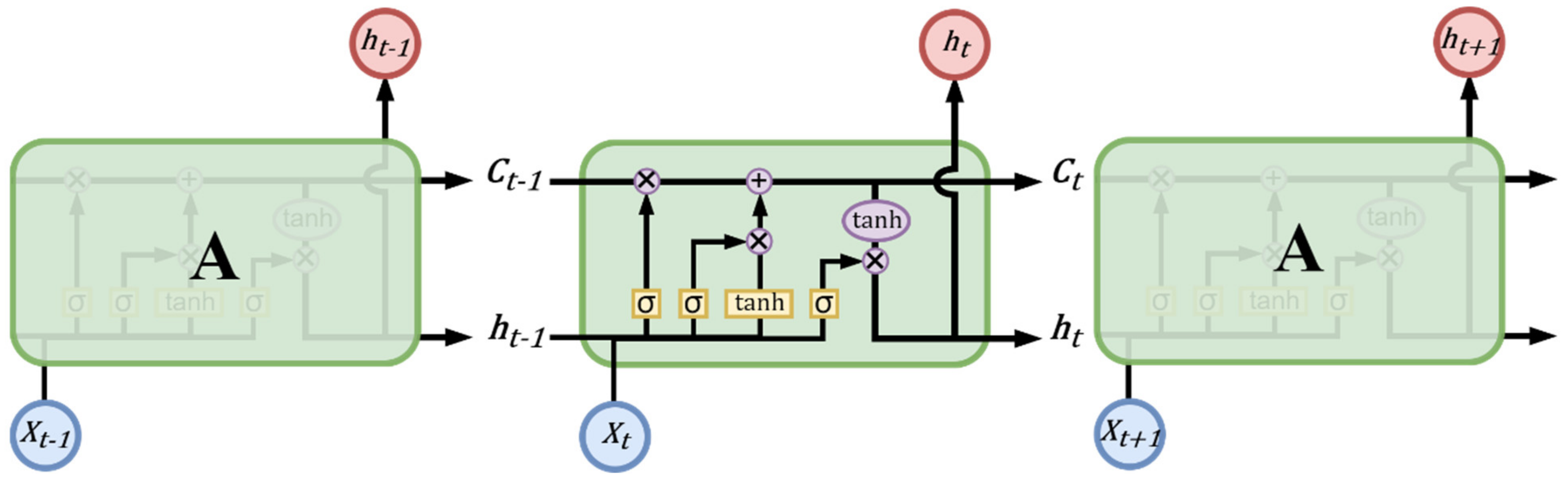
As shown in Figure 3, it can be found that the structure of LSTM is much more complex than the structure of RNN. In general, the internal structure of the RNN reuses a neuron, for example, a tanh layer. LSTM consists of three gates: input gate (i_t), output gate (i_o) and forgotten gate (f_t), and a memory cell to gate, to control the message added to the memory unit and removed from the memory unit, so that these three switches are used to protect and control the memory state; they have their respective weights and will be weighted according to the input data. After calculation, each switch decides whether it is on or off.

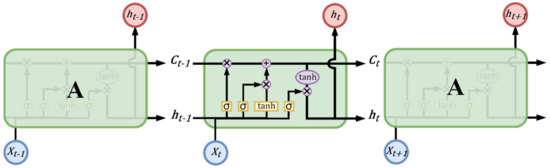
Figure 3. LSTM basic architecture diagram.

Due to the unique design structure of LSTM, the state generated by the previous input data can be stored in the memory space through a temporary memory space in neurons. Different output values are calculated. The operation and calculation method of each gate are described below.

First, you need to decide that messages should be discarded in memory cells, such as Equation (7). If the timing is t, W means the weight matrix, h_t−1 is the output at time t−1, x_t input for time t and b_f represents the bias value. Converted through the sigmoid layer, these will result in values between 0 and 1. The value 1 is fully reserved, 0 is completely discarded and the final forgotten gate the output is represented by f_t.

$$f_t=\sigma \left(W_f·\left[h_{t-1},x_t\right]+b_f\right)$$

(7)

Again, one needs to decide which new messages to save into the memory unit and split into two parts, adding temporary states and updating old states. For example, in Equations (8) and (9), i_t determines which values need to be updated through the sigmoid layer, and ${\tilde{C}}_t$ creates a vector through a tanh layer with new candidate values. These two results are updated in the Equation (10), where W_i, W_c represents the weight matrix and multiplies the old state C_t−1 by f_t to determine the need to forget the message, plus the new candidate value i_t·${\tilde{C}}_t$, will be in the new state C_t, b_i and b_c, which are the bias value.

$$i_t=\sigma \left(W_i·\left[h_{t-1},x_t\right]+b_i\right)$$

(8)

$${\tilde{C}}_t=tanh\left(W_C·\left[h_{t-1},x_t\right]+b_C\right)$$

(9)

$$C_t=f_t·C_{t-1}+i_t·{\tilde{C}}_t$$

(10)

Finally, one needs to decide the output message, such as the Equations (11) and (12), by means of a sigmoid layer to determine which parts need to output o_t from the memory unit, and the state of the memory unit is passed After the tanh layer, one obtains a value between −1 and 1, multiplying o_t with $tanh\left(C_t\right)$ and finally the h_t to determine the output. Where b_o is the bias value.

$$o_t=\sigma \left(W_o·\left[h_{t-1},x_t\right]+b_o\right)$$

(11)

$$h_t=o_t·tanh\left(C_t\right)$$

(12)

2.5. Bidirectional RNN (BRNN)

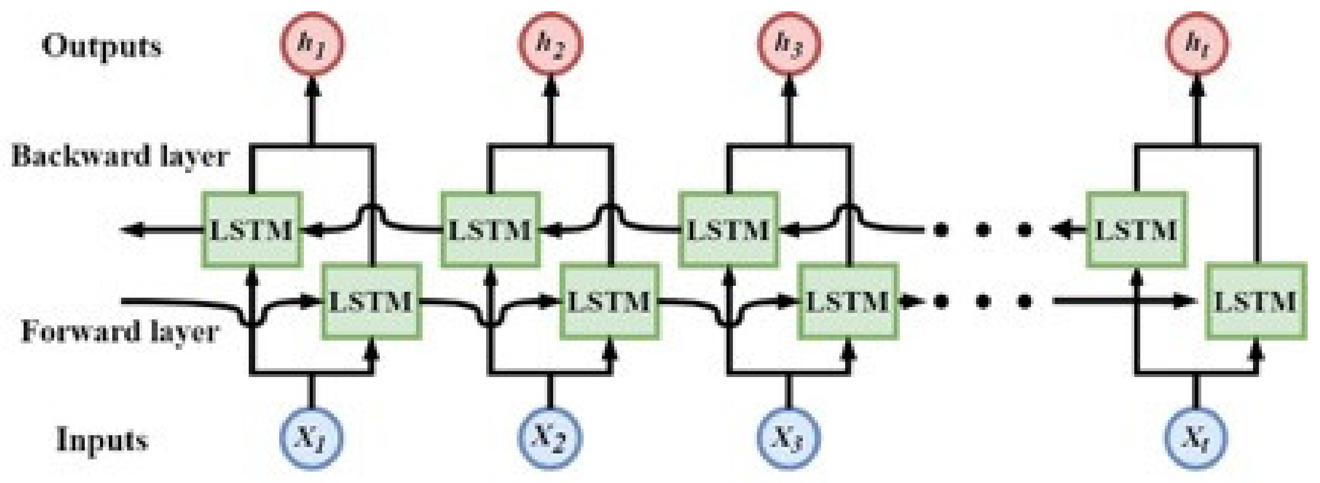
Traditional unidirectional RNN predict the next moment of output only based on previous messages, but in many cases the current output is not only relevant to the state of the previous moment but also to the future status that is related. For example, when we predict missing words in a sentence, we need not only to judge from the previous narrative, but also to consider the latter. Therefore, BRNN [33] can take advantage of both the pre- and post-message in the text.

Figure 4 shows a schematic diagram of the BRNN network. In the BRNN model, each training sequence has two circulating neural networks, each connected to a single output layer, one backward and one forward. During training, training materials are imported into the model in both directions. Input messages for both directions are stored in the hidden layer where the corresponding output is connected to the corresponding output layer, and the final output is determined by the status of the two RNNs.

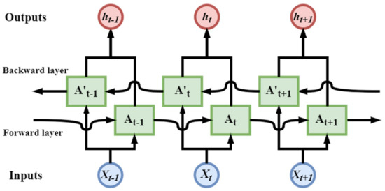
Figure 4. Schematic diagram of BRNN network architecture.

In the case of so many models being used, one should choose an algorithm model suitable for the application of this paper. Because this paper uses the object detection model to grab the movement trajectory of large cars at intersections, it is necessary to use a more immediate, simple, fast and accurate object detection network model, Faster R-CNN, which is a common object detection method, but the detection speed is too slow, about 7 frames per second (FPS), although it is very accurate for detect objects; this algorithm technique is too complex for beginners using deep learning. Therefore, it tends to use YOLOv4 in detecting smaller objects, compared to the previous generation YOLOv3, the accuracy and speed has a relative improvement, and this algorithm is very fast, with the use of a lightweight network. The architecture can be computed up to approximately 400 FPS on the GPU.

When we look at the object’s independent trajectory patterns, objects in different motion modes have different velocities, acceleration and gait movements. To predict the trajectory of the target object’s movement, the key is to analyze the target object’s time information in the time series in the image and accurately predict the target even in uncertain and unpredictable situations in the future movement trajectory. In order to achieve this prediction, this paper uses RNN to predict the trajectory by comparing multiple models and selecting a bi-LSTM with a high accuracy of bi-LSTM.

3. System Architecture

Because large cars and locomotive knights in the inner wheel difference accident is often at the turn of the junction, through the installation of video equipment at the intersection, for the perspective of locomotive and bicycle image collection, and with deep learning machine vision to detect the movement of large vehicles, it is important to predict the movement trajectory of inner wheels when turning the large car in the intersection. This paper expects to predict the movement trajectory of large cars in the next few seconds by analyzing the intersection images collected.

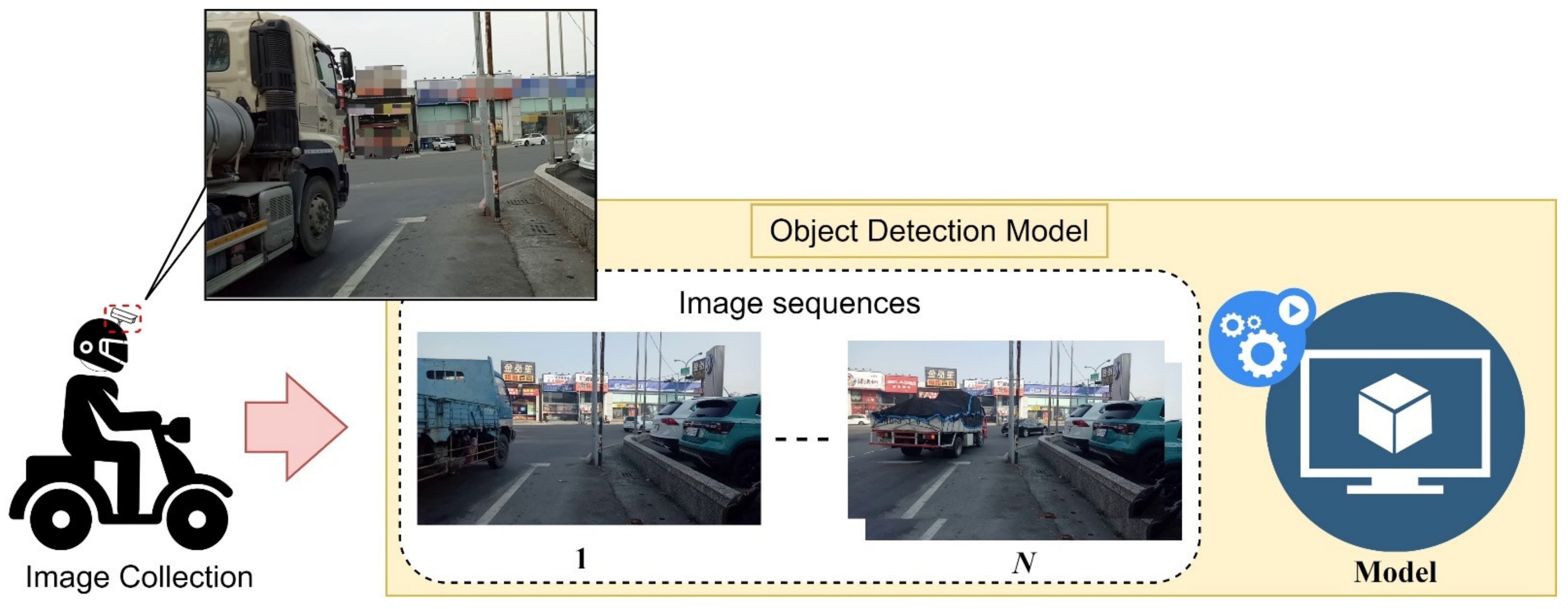
In the schematic diagram in Figure 5, showing the system architecture, the system can be roughly divided into three module blocks, the data collection module and object detection module, and the trajectory prediction module. The data collection module mainly collects moving images of large vehicles at intersection and provides the object detection module for training and testing and finally passes the results to the trajectory prediction module for training with predicting the trajectory of a large truck at the intersection when turning.

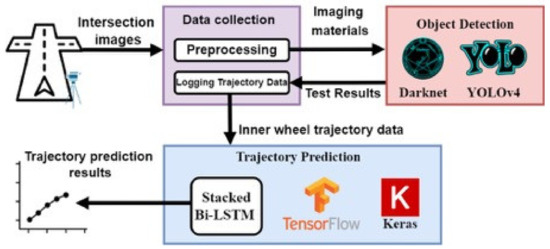
Figure 5. System Architecture Diagram.

In Figure 6, the locomotive rider system uses the situation in the locomotive or driving helmet set up tachograph and the data collection. Data collection was conducted mainly through the perspective of the locomotive knight to set up a drive recorder or set up video equipment at the intersection of the same height, in order to collect the moving images of large cars at the intersection; the images will be taken according to the truck time segmented, in addition to collecting a variety of large car images from the web from the web crawlers. The image data is provided to the object detection module for model setup and training.

Figure 6. Motorcycle knight system usage scenes.

During object detection through the use of Darknet framework for YOLOv4 object detection model training, it is mainly adapted for training images, training different numbers of images in batches, and finally, for testing the model. The network detects whether the accuracy allowed by the system is reached. trajectory prediction contains a bi-LSTM bidirectional circulating neural network model built using TensorFlow, which mainly modulates the detected object movement trajectory data and will adjust trajectory data that is randomly placed into the model for training to predict the movement trajectory when a truck turns at an intersection.

3.1. Data Collection

The images that can be collected at the traditional intersection are usually taken by the intersection or store monitor. It is difficult to collect images from the viewpoint of the road by the locomotive knight or pedestrians. Video data at the turn is to be erected at the same height as the locomotive knight viewing angle at the side of the road to observe and collect actual trajectory data.

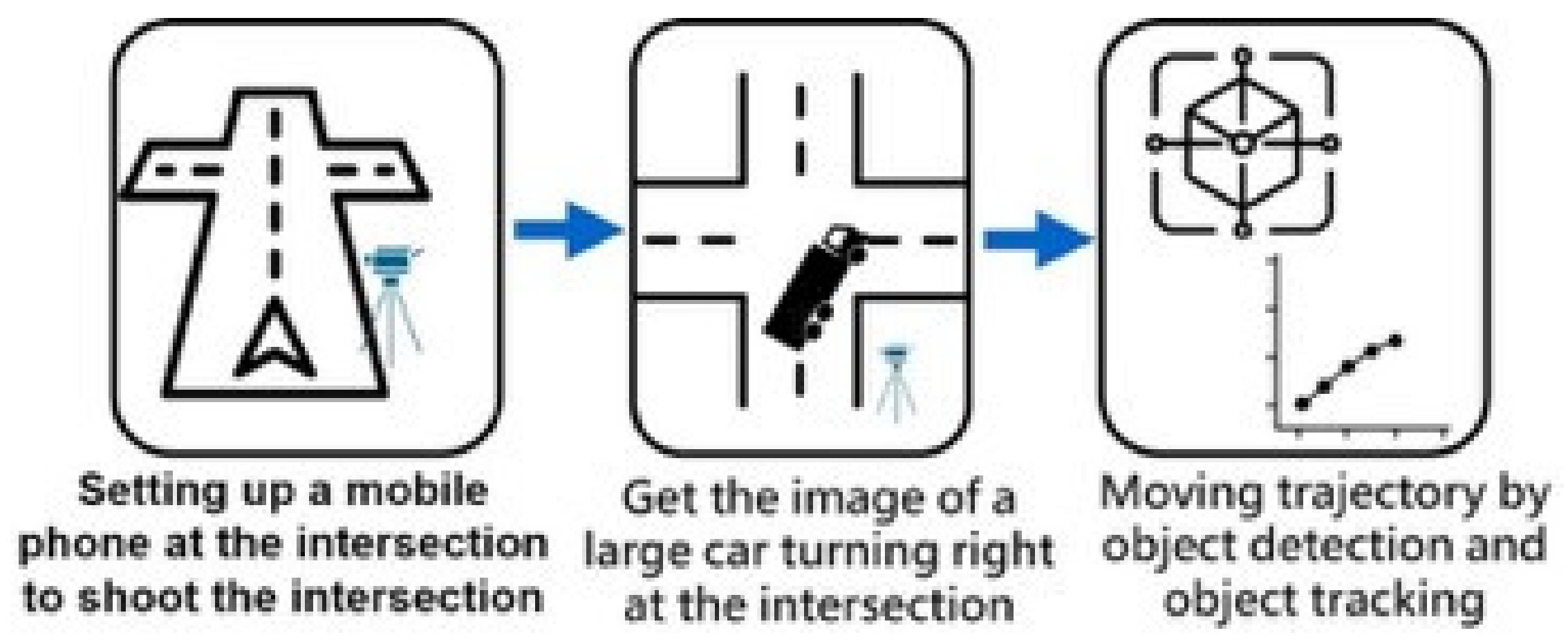
The data collection process is shown in Figure 7, as a large car turning trajectory data collection process diagram, first in the intersection of large cars through the intersection of mobile phone shooting, in order to collect intersection images. The video taken at the intersection is segmented according to the time of the arrival of the truck, with the segmented image placed into the object detection model of “object detection” and “object tracking”, and the corresponding pixel is coordinated. According to the time record, the inner wheel movement trajectory of large cars at the intersection is obtained for training and prediction of trajectory prediction models. At the same time, the collected large car images are labeled, and the large car figures collected by web crawlers are put into the object detection model for training.

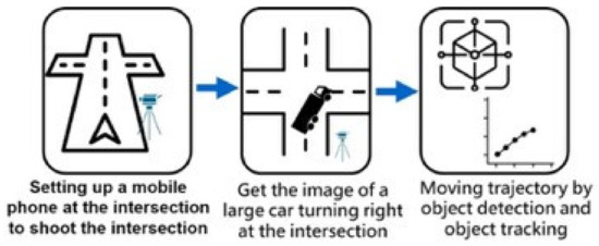
Figure 7. Schematic diagram of the data collection process of large car turning trajectory.

• Object detection

For detecting objects in the captured image, we apply YOLO for vehicle detection and YOLO detection results, e.g., object name, image coordinates, detection confidence index, and create a new object list and record the information for each frame.

• Object tracking

YOLO and other object detection algorithms are all operations on each frame captured by the camera. If the objects detected are counted directly on each frame, the same objects will be counted repeatedly; in order to avoid this happening and to use object tracking technology to distinguish the information of each frame, compare the x, y pixel coordinates of the center of the bounding box before and after the frame, and the coordinates of the next frame to the previous frame coordinate the European distance operation. The shortest European distance can be considered as the same object.

On the road, unless the same object leaves the detection range or is obscured by other scenes, there is basically no sudden disappearance of the object. Thus, in the comparison between the front and back frames, the coordinate distance between the image of the object is detected and the previous frame is not too far apart. This paper uses the storage front frame data to compare with the rear frame data to see whether the same object is still in the detection range. First, using the YOLO object detection model to detect each frame of the captured image, store the object information in a list form, and continue to receive the next frame content, comparing the bounding box center of the two frames before and after. The last frame list is used as a benchmark to find the object that is the shortest distance from the current frame, so that the comparison results are the same object.

Such as the Equation (13), for calculating two points in the list (x₁, y₁), (x₂, y₂), …, (x_t, y_t) to coordinate the difference, this paper uses Euclid distance (also known as European distance) to calculate the straight distance of the shortest line between two points. Where d is the Eujid distance of the current frame (x_t, y_t) from the previous frame ($x_{t-1}$, $y_{t-1}$) of the coordinate point, find out the center of each bounding box appearing in the image, which is the point with the shortest distance from the center of the previous bounding box, in order to set a threshold in several calculations. If the calculated distance is greater than 30 pixels, it means that this result is a newly detected object: A new list is created for this object to store the next frame. For recording data and comparisons, if the pixel quality is less than 30, the test result is the same object, and the results are added to the established list. If the target disappears and the list is not updated, the data of the objects recorded in the list is exported and the list is deleted.

$$d=\sqrt{{\left(x_t-x_{t-1}\right)}^2+{\left(y_t-y_{t-1}\right)}^2}$$

(13)

3.2. Object Detection Model

There are many neural network models for object detection, but the system in this paper needs to balance the accuracy and speed of detection execution; therefore, it is necessary to choose both to reach that are within an acceptable range. After comparing the results of various object detection neural network models with the use of FPS and YOLO, an object detection model with a high average accuracy will be selected.

In machine learning, one will need to collect different training materials as much as possible in order to avoid overfitting the model. This issue causes the model to be more accurate for the checked data detection and vice versa. In addition to this, consider the resolution and size of the image: the higher the resolution, the more information one can take from the image. This paper plans to search for different types of objects, shooting angles, ambient light and environmental complexity from the network to increase the awareness of neural network models.

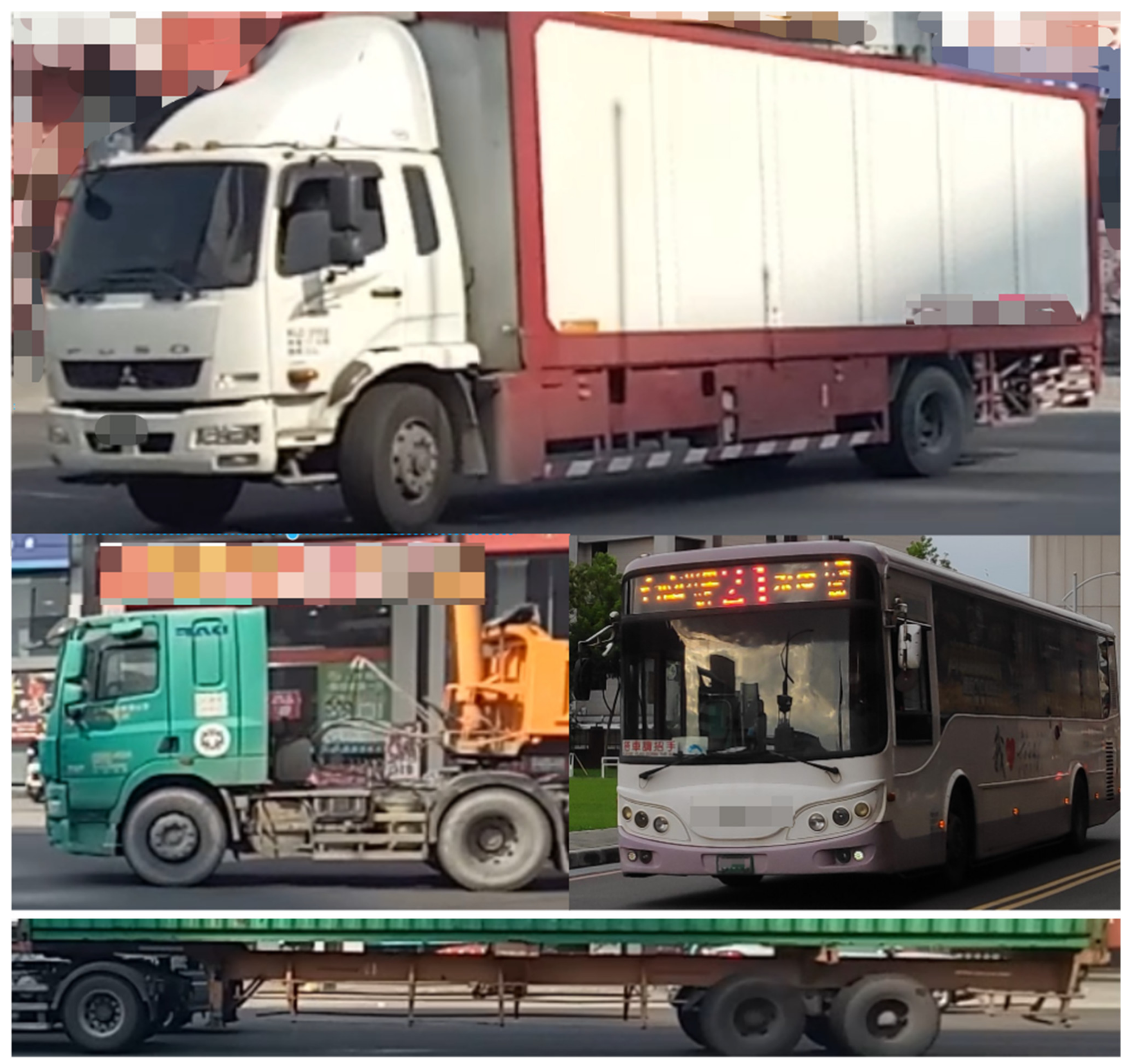
In addition, in order to simulate the actual scene, a mobile phone is set up at the intersection where large vehicles are frequent. The size of the image needs to be selected, and should not be too small or too large. This paper plans to re-scale the collected images to 1280 × 720 and add images of about the same size on the web to be used as training materials for the model. Figure 8 shows a schematic of the types of training images collected, which include trucks, buses, tractors, semi-linked vehicles and semi-linked vehicles, and are combined with the bottom semi-trailer.

Figure 8. Schematic of the type of training image.

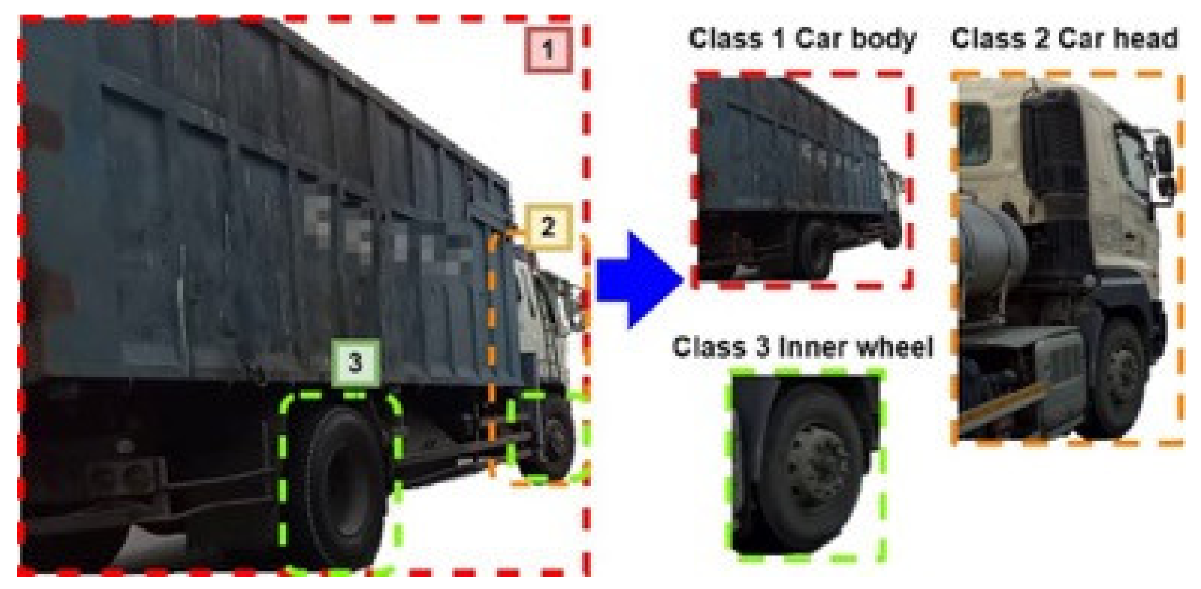
Next, one needs to determine the type and scope of the object classification in the image data. Use LabelImg [34] labeling tool LabelImg [34] to perform manual labeling. Figure 9 shows the training image analysis diagram. It is important to pay attention to the selection of categories in addition to large cars needed to label their front and wheels. The main purpose is to grab the range of contact with the pavement when turning large cars, which need to grab the image of the movement of large car tires and avoid detection with other objects prone to error, for example: other types of tires. In addition, the information generated by the labeling process has a great impact on the accuracy of the training model detection. Thus, one needs to note that the process needs to be marked with a human eye view.

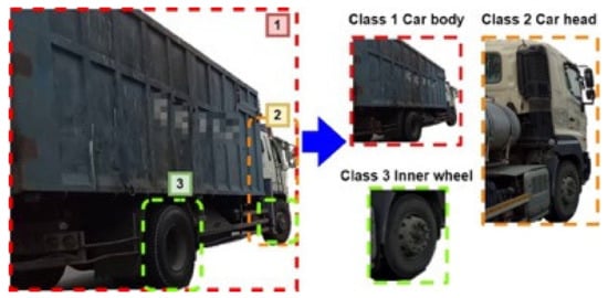
Figure 9. Schematic analysis of the training image.

We label the image 1, 2 and 3 for three objects; after the image labeling, we produce the corresponding TXT file, which is used to store the content of the labeling image. Its content contains the label category name of x, y, w, h, which is composed of four values, where x, y represents the ratio of the center coordinate of the label image to the width and height of the image. w, h represents the ratio of the width and height of the label image to the input image width and height. If the image is too blurred, causing the object to lose its features, the object is shaved.

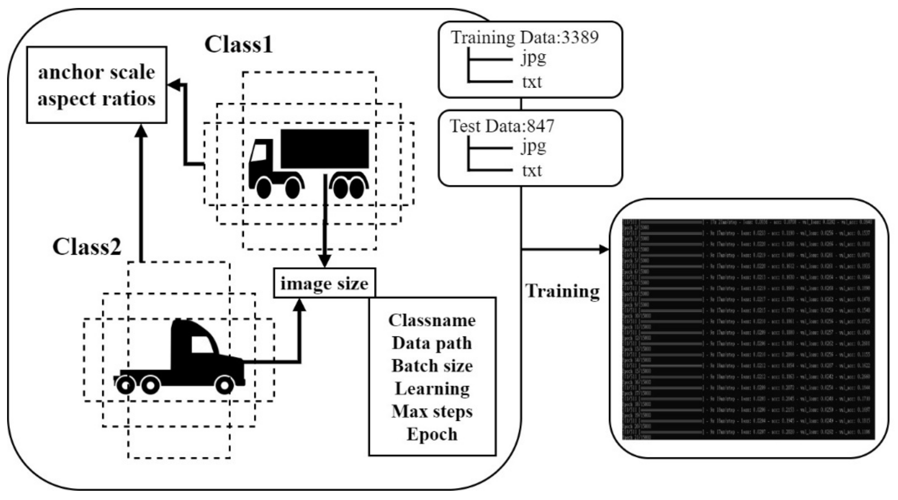
Before starting the training model, one needs to configure the environment parameters for Darknet to construct the neural network model, as shown in the Figure 10 training file setup diagram, including the number of categories, image input size, the maximum minimum scale of the bounding box produced by anchor, the number of batch trainings and the number of rounds of training. Whereas, the amount of batch training is determined by the size of the memory space of the GPU and affects the overall convergence rate of the loss Value to RTX 1080, one sets the batch number of 24 images to be based on 8 G.

Figure 10. Schematic of training profile setup.

In order to observe the stability of the neural network model, the number of training steps is set to 15,000 rounds, and the prepared images will be randomly selected at a ratio of 2:8, with 20% of the data as test images and 80% of data as training images. After training the model, the converted data will be automatically poured into the model according to the parameters set. After training, the test image is cross-validated, and the result is displayed on the terminal to view the loss of the change of function.

Figure 11 shows Darknet using a folder structure diagram. Although Darknet can directly and quickly build neural network models, the data structure is too complex and can cause it to be difficult maintain and build the model, which creates three directories under the Object Detection directory, and places the train_data and val_data directories to be used for training and testing image data, corresponding to the txt file, which records the coordinates of the category and bndBox indicated after the image is labeled.

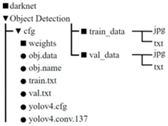
Figure 11. Schematic diagram of Darknet using a folder structure.

3.3. Trajectory Prediction Models

In general, our forecasts of time series data require data in the past, and future data are essential, resulting in a significant impact on the accuracy of the forecast. In addition, RNN is prone to gradient disappearance or explosion problems during training. LSTM, which is used to solve gradient explosion and loss of gradient during long sequence training, is the prediction. However, in some problems, the output of the current moment is not only related to the previous state, but also to the future state. After comparing multiple models, the higher accuracy of double Bi-LSTM makes predictions.

Here, we explain how to deal with the captured intersection image file, and import the file into the object detection model, as shown in Figure 12, which is the data collection diagram of large vehicle movement trajectory data, shown through the object detection model to detect large vehicles to obtain the position of the front and rear wheels in the image. The red dot represents the movement of the large front wheel; the rear wheel is represented by the blue dot.

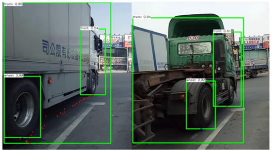
Figure 12. Roadmap of moving trajectory data collection of large vehicles at intersection.

Note that some large vehicles do not have only one set of rear wheels; thus, the object tracking method will determine whether the rear wheel is the last set of wheels of a large car, in this way obtaining the large car at the intersection When turning, the actual moving trajectory data of the front and rear wheels contact with the road, and set the sampling frequency of data to 10 Hz, and 10 trajectory coordinates per detected target every 1 s. Some of the data are found to have incorrect track coordinates; thus, the wrong coordinate data will be preprocessed.

Figure 13 shows the trajectory data of a large car in the intersection movement data. Each color represents the trajectory data of a group of large cars at the intersection, which is visualized by the data. The map can observe each car at the same intersection of the movement of different trajectories, and also finds some wrong trajectories in the figure.

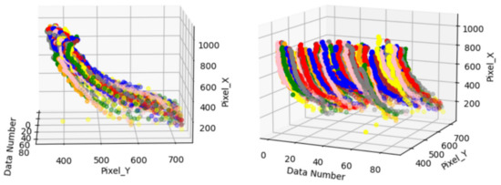
Figure 13. Visualization of moving trajectory data of large vehicle intersection.

Figure 14 shows a diagram of the data preprocessor. In order to find the wrong trajectory, the pixel coordinate F(x_t, y_t) of the front wheel and the rear wheel pixel coordinates W(x_t, y_t) in the original data, one divides and calculates the vectors between the coordinates separately to find significant outliers, and finally removes the outliers and makes up the average of the two points as the value of that coordinate.

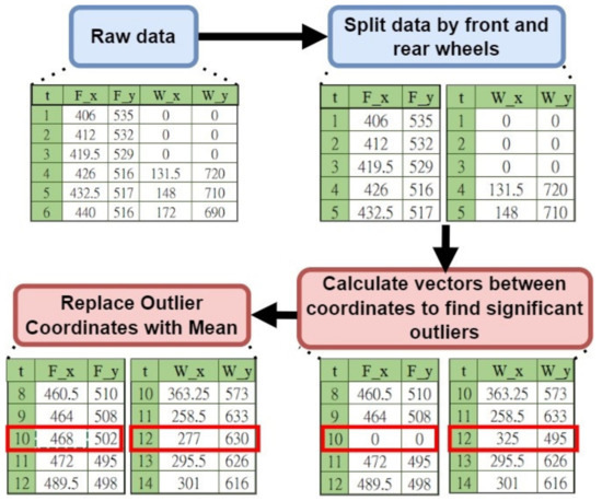
Figure 14. Schematic diagram of the data preprocessor.

The method proposed in this paper is to stack two layers of Bi-LSTM with the Stacked Bi-LSTM structure as a hidden layer. Figure 15 shows a single layer Bi-LSTM architecture diagram; the single layer Bi-LSTM consists of two layers of the green block LSTM structure, with one layer for backward training tasks and the other for reverse training tasks. In addition, the layer uses 240 neurons, the timing information is input from left to right, X₁, X₂, …, X_t represents the input data for each time sequence, h₁, h₂, …, h_t for each time sequence the output of a layer of Bi-LSTM and t represents the input time.

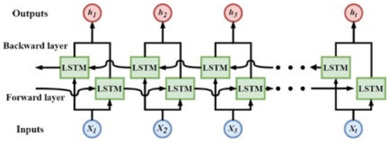
Figure 15. Schematic diagram of single-layer Bi-LSTM architecture.

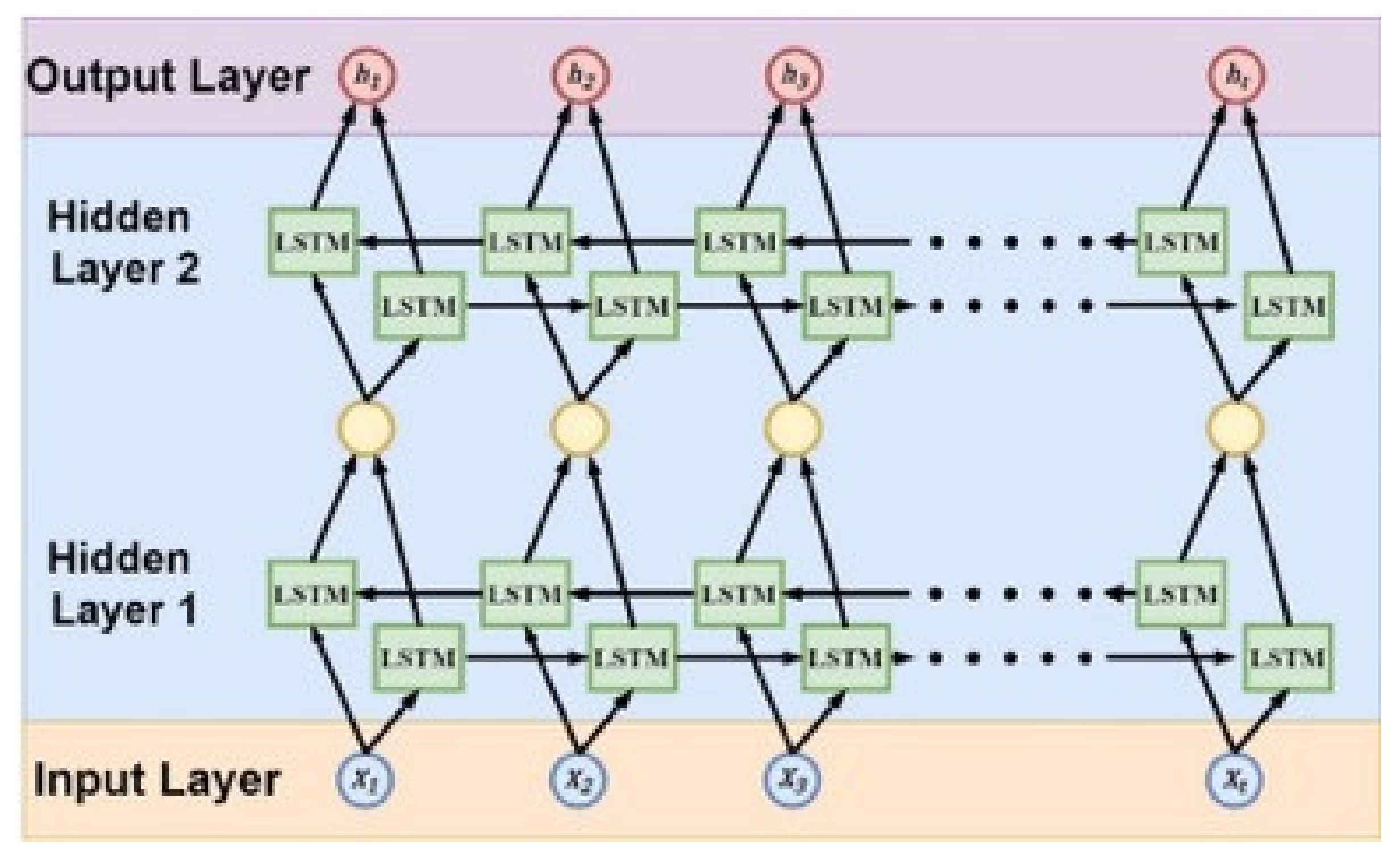
Figure 16 shows a schematic diagram of the Stacked Bi-LSTM architecture. After the input data passes through the first layer of Bi-LSTM, the output of each time series will be used as the second layer Bi-LSTM input data, and it is output in the same way as the second layer, which belongs to the architecture of Many-to-Many in LSTM. The reason for this is because the purpose of this paper is to predict the movement trajectory in the next few seconds, not just where it occurs after a few seconds.

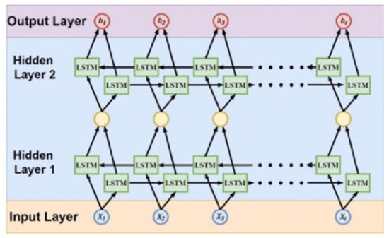
Figure 16. Stacked Bi-LSTM architectures.

In order to improve the learning speed of the network model and avoid the overfitting problem of neural network during training, before putting the data into the model training, the input data will be normalized in advance, and the value will be output between 0 and 1. So, this improves the comparability of the training data. We also join the dropout to avoid the overfitting of neural networks. The dropout will randomly delete neurons, which can reduce the dependence between neurons; thus, the model will not rely too much on a neuron, by reducing the network complexity and effectively prevent overfitting.

In this paper, the Stacked Bi-LSTM neural network is used; one mainly adjusts the parameters of the neural network training through the rules of thumb. The excitation function of the model as ReLU is set based on the rule of thumb, and the optimizer uses Adam. Its advantage is that after bias corrections, the learning rate of each iteration has a certain range, making the parameters more stable. We observe the change of the loss value and adjust the parameters of the model, and only adjust the parameters of one neural network at a time.

The experiment in this paper was trained on a trajectory prediction model with GPU using the Keras suite on TensorFlow. The trajectory prediction model training parameters take the display card GTX 1080 8 G as an example. The optimizer used is Adam and loss function is mse. The Adam optimizer updates weights in the neural training model based on the loss value and updates the weights in the neural training model based on the loss value. In addition, in each layer of the Bi-LSTM the dropout layer is added, to a dropout value of 0.5, in order to randomly remove several neurons for training to prevent neural network overfitting, and finally to add flattened and fully connected layers (Dense).

In the input layer section, one needs to set a fixed time series length (timestep), which represents the fixed length of each time the data is dropped, as well as the input data dimension. In the training set, this paper takes the smallest number of data pens in all turn trajectories as the timestep length, assuming that there are 50 large car trajectory data in the training set; therefore, including the smallest number of data pen, the number of trajectories is 30, and the training set input timestep is 30.

This setting ensures that most of the data can be trained, and that input data within the timestep length will be trajectory data of the same vehicle, in accordance with the nature of the predicted timing information, because of this type of method. The data in the training set need to be cut or complementary in the timestep length. For example, the timestep is set to 30, then, each trajectory data will be based on every 30 trajectory coordinates. Cutting, which abandons the rest according to its set threshold, such as: a trajectory data with 95 trajectory coordinates where the threshold is set to 20, then, it will be cut into 3 segments; the neural network reads a section of information each time in each segment. There are 30 areas of information, while the remaining 95 – 30 × 3 = 5 information is discarded.

4. Results

The main purpose of this study is to identify and predict the inner wheel trajectories of the front and rear wheels of large vehicles turning at an intersection from the perspective of motorcycles and cyclists. Therefore, when collecting data, we need to find the intersection where large vehicles often drive, and take photos without affecting road safety. It takes a lot of time to find the shooting location, take images and sort out image data.

In this study, a total of 33 h of images were collected at the intersection. The images of large cars turning at the intersection were taken out in sections, and the parts in which the wheels in the large car were not obscured by other objects, and with clear images, were selected as the training data of object detection. Finally, the trained object detection model is used to detect the moving track of the inner wheel of the large car in the image, which is used as the track data of the track prediction model. A total of 374 groups of the large car trajectory data were screened and put into the trajectory prediction model for training in the proportion of 8:1:1.

This paper plans to use an object detection model to detect large vehicle images and their front and rear wheel positions on images in order to apply the results to predict the movement trajectory of large cars at the intersections. Because of the differences of different neural network models, this paper will be the same as the training materials, respectively, in YOLOv4, YOLOv3 and the MobileNetv2 SSD object detection model, with residuals of the Network Resnet152 serving as a faster R-CNN of the basic network model and comparing its training results.

The experimental training parameters, such as in the Table 3 neural network model setting table, demonstrate that the above four methods will be trained with the same information. In the training materials, videos taken at the intersection were sampled at 10 Hz, and 3389 images were already marked as training sets, with 847 images taken from the highlighted data as the test set for the model; the training results are described below.

Table 3. Neural network model setup.

Names	Parameter Value
Training image size	512 × 512
Number of training images	3389
Number of classes	3
Learning rate	0.003
Maximum number of training steps	15,000
Number of training	A total of 3389
Number of tests	A total of 847

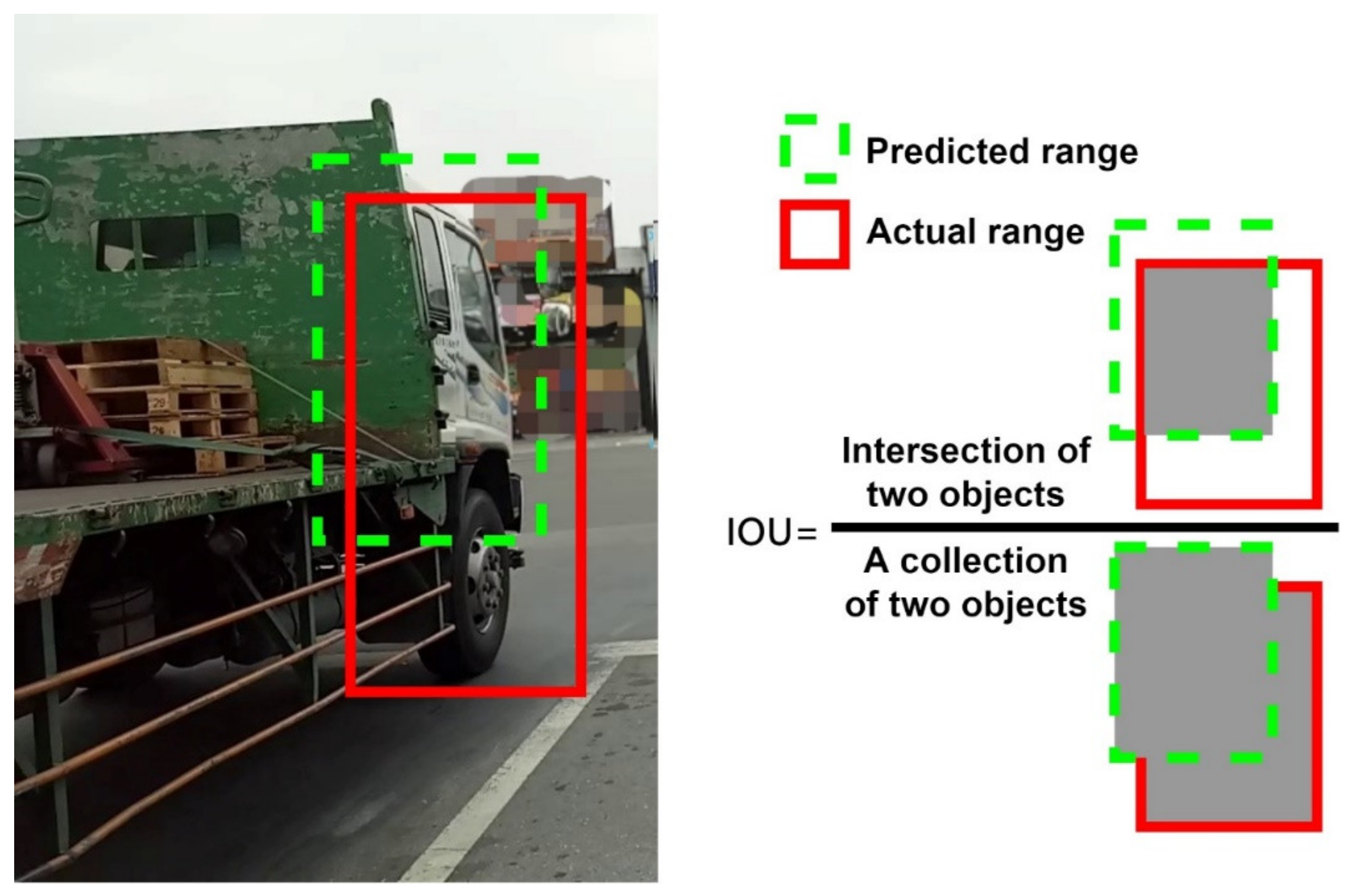
This experiment is divided into three categories, with the whole truck called “truck”, the front of the truck called “front” and the wheel of the truck called “wheel”. For the object, the accuracy (Average Precision, AP) and mean accuracy (mAP) predicted by each category are recorded separately when the model is trained. The accuracy prediction is greater than the 0.5 intersection over union (IOU), for example. Figure 17 illustrates the IOU with the category “front” as an example.

Figure 17. IOU interpretation schematic.

In order to find suitable object inspection models, this paper builds four object detection models and is trained under the same conditions, such as the Table 4 object detection model comparison table. YOLOv4 is an object detection model.

Table 4. Comparison of training results of object detection models.

Model Name	Image Size	Truck AP	Front AP	Wheel AP	Average Accuracy (mAP)	(GTX 1080 ti 8 G) FPS
ResNet152 Faster RCNN	512 × 512	72%	83%	61%	72%	6
MobileNet ver2 SSD	512 × 512	85%	90%	77%	84%	39
YOLO v3	512 × 512	90%	89%	85%	88%	49
YOLO v4	512 × 512	98%	97%	96%	97%	55

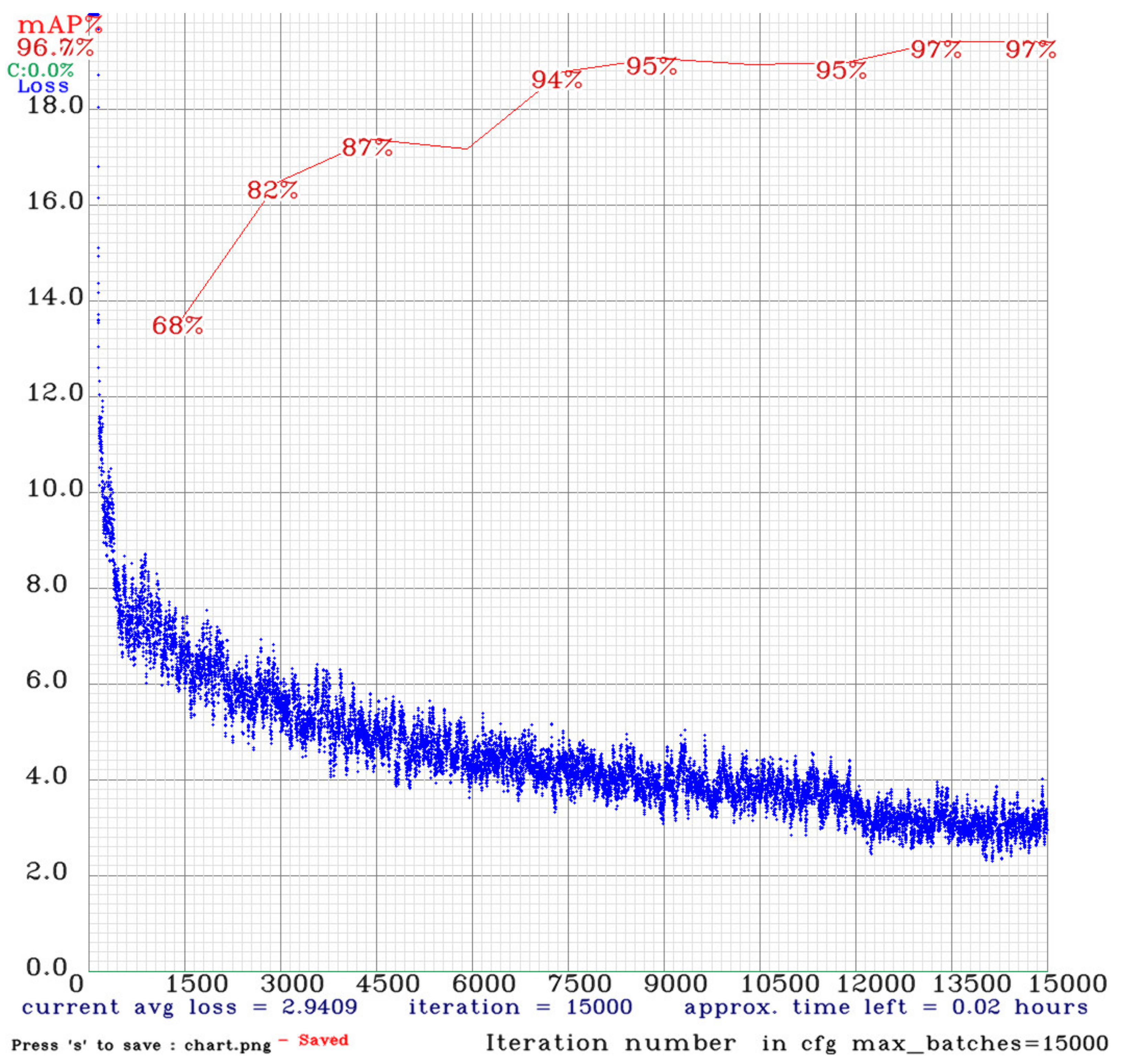
The training process is shown in the YOLOv4 training curve in Figure 18, which demonstrates the early stages of the training to drop quickly, due to a higher learning rate at the beginning and after a period of training. The Learning rate is gradually reduced to avoid oscillation. When the training steps close to 1500, the loss drops below six to start calculating the mAP value. The mAP value curve continues to grow and is inversely proportional to the loss curve, indicating that training is good, with no overfit occurring, and the model begins gently when the training steps approach 4500 steps, approximately when the 12,000 step start model is nearing saturation and the overall model training time is about 7.5 h.

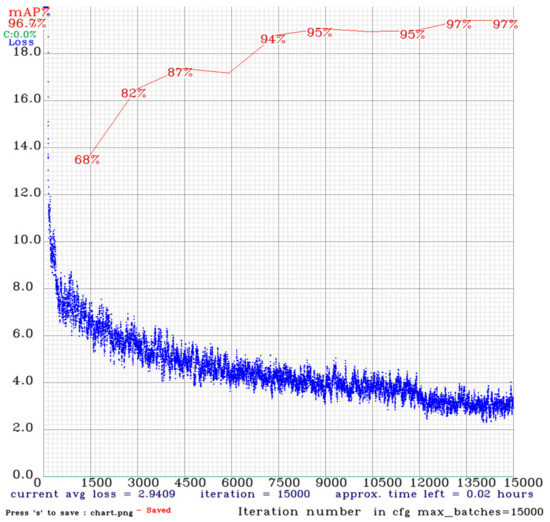
Figure 18. Training curve of YOLOv4.

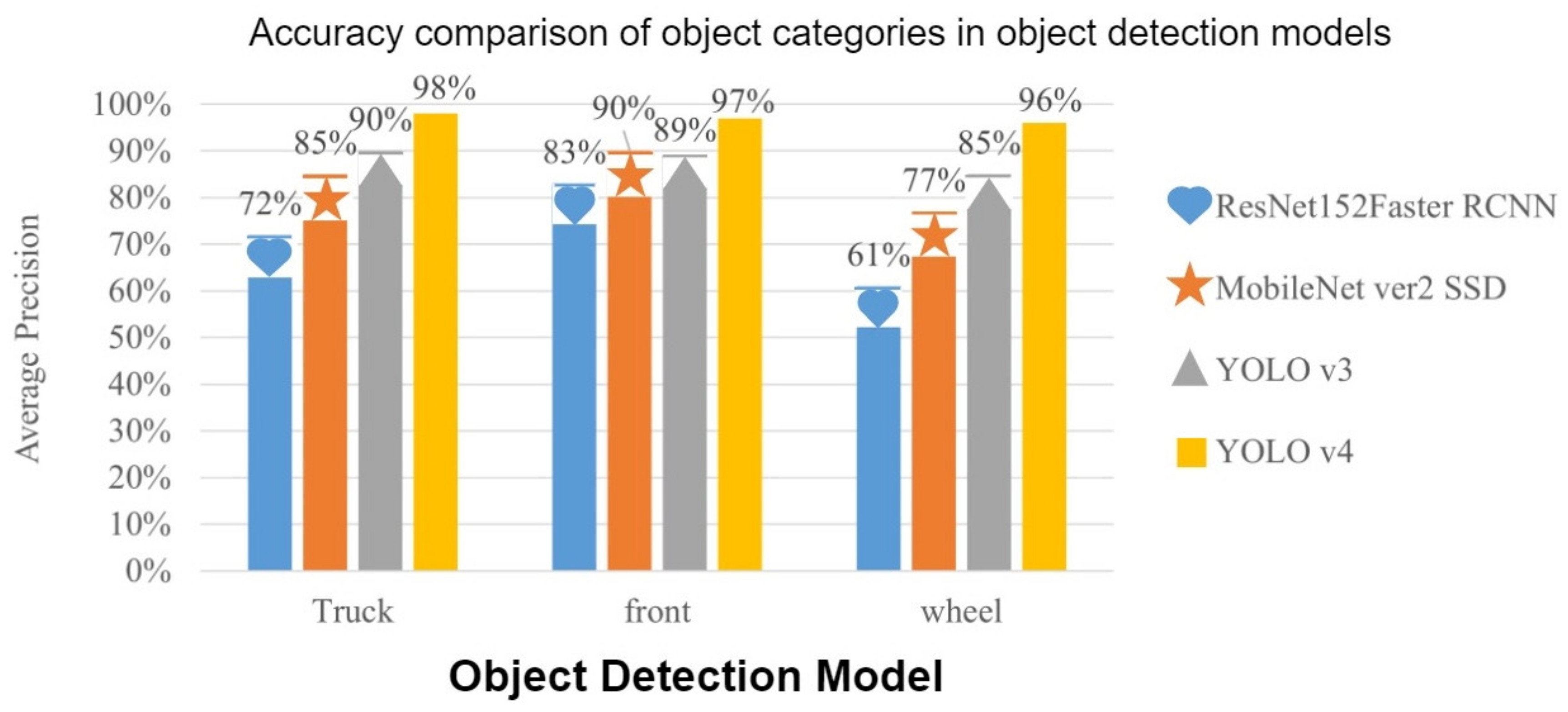
In the training results shown in the comparison table of the object detection model in Table 4, the categories are compared and the growth bar plots are drawn. From Figure 19 it can be found that YOLOv4 accuracy in three categories is higher than other object detection models. In addition, Figure 20 compares the average accuracy (mAP) in each model with the frames per second (FPS), and the YOLOv4 average accuracy and FPS are also higher than other models.

Figure 19. The accuracy of object detection of various categories is relatively long.

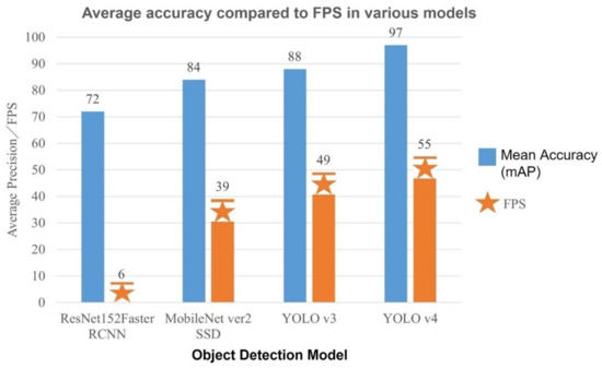
Figure 20. Object detection average accuracy and picture update rate comparison.

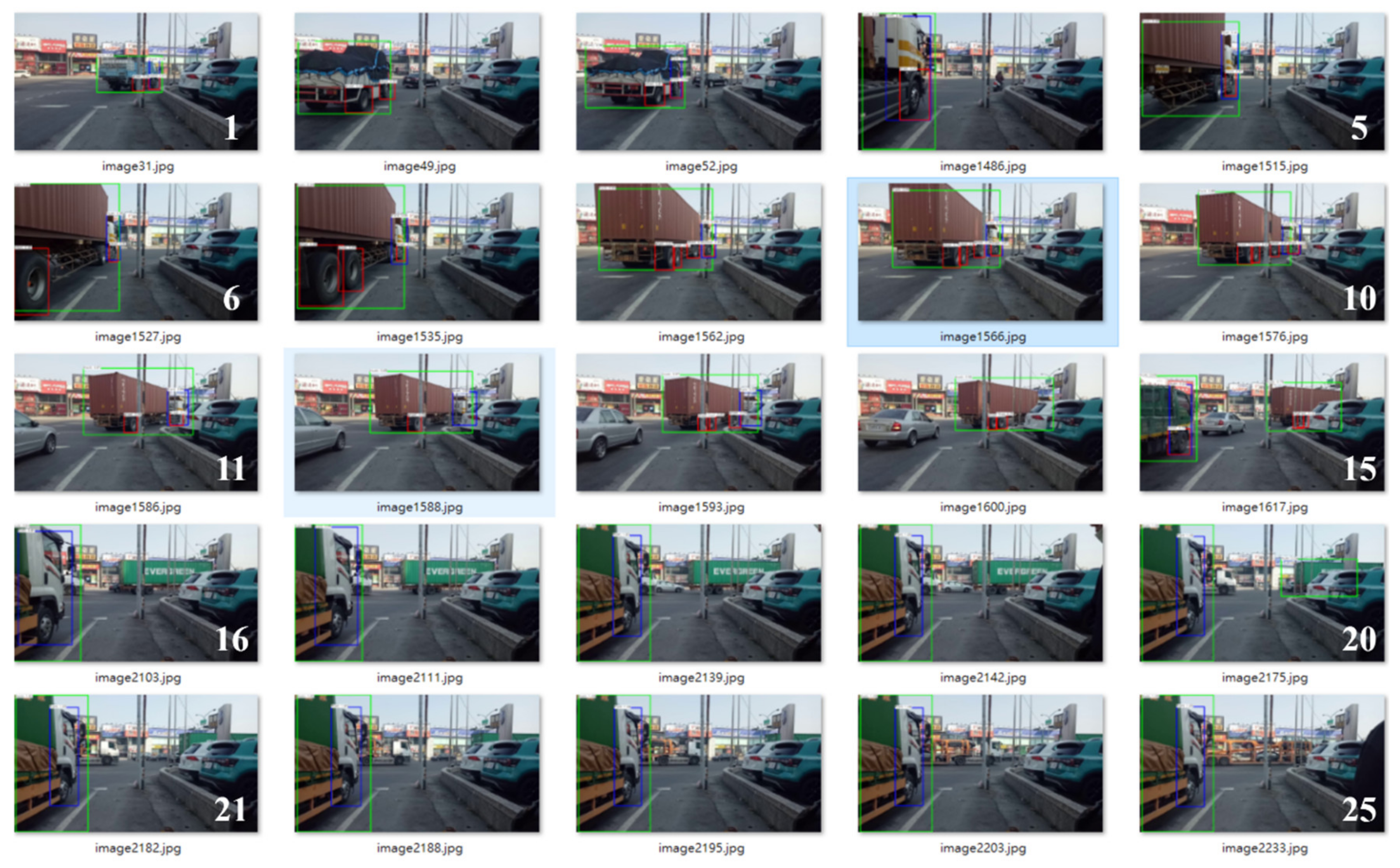
As shown in Figure 21, Figure 22 and Figure 23, the object detection neural network model training is completed, the random capture of 74 images from the untrained images will be executed in the model and the green box represents the category truck, with blue for the category front and red for the category wheel. In general, the objects are clear or less obscure, can be easily detected in the image and all categories are the same. However, in the lack of light with too much masking, the objects are too small on the image or objects. Too many similar colors can result in incorrect detection.

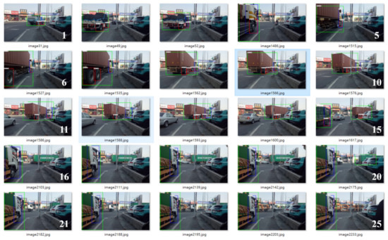
Figure 21. Test image (1~25).

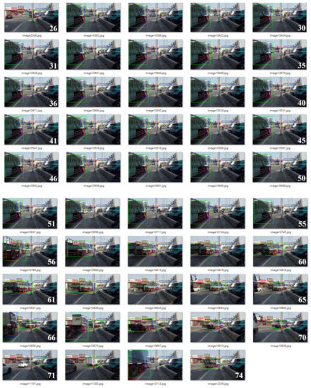
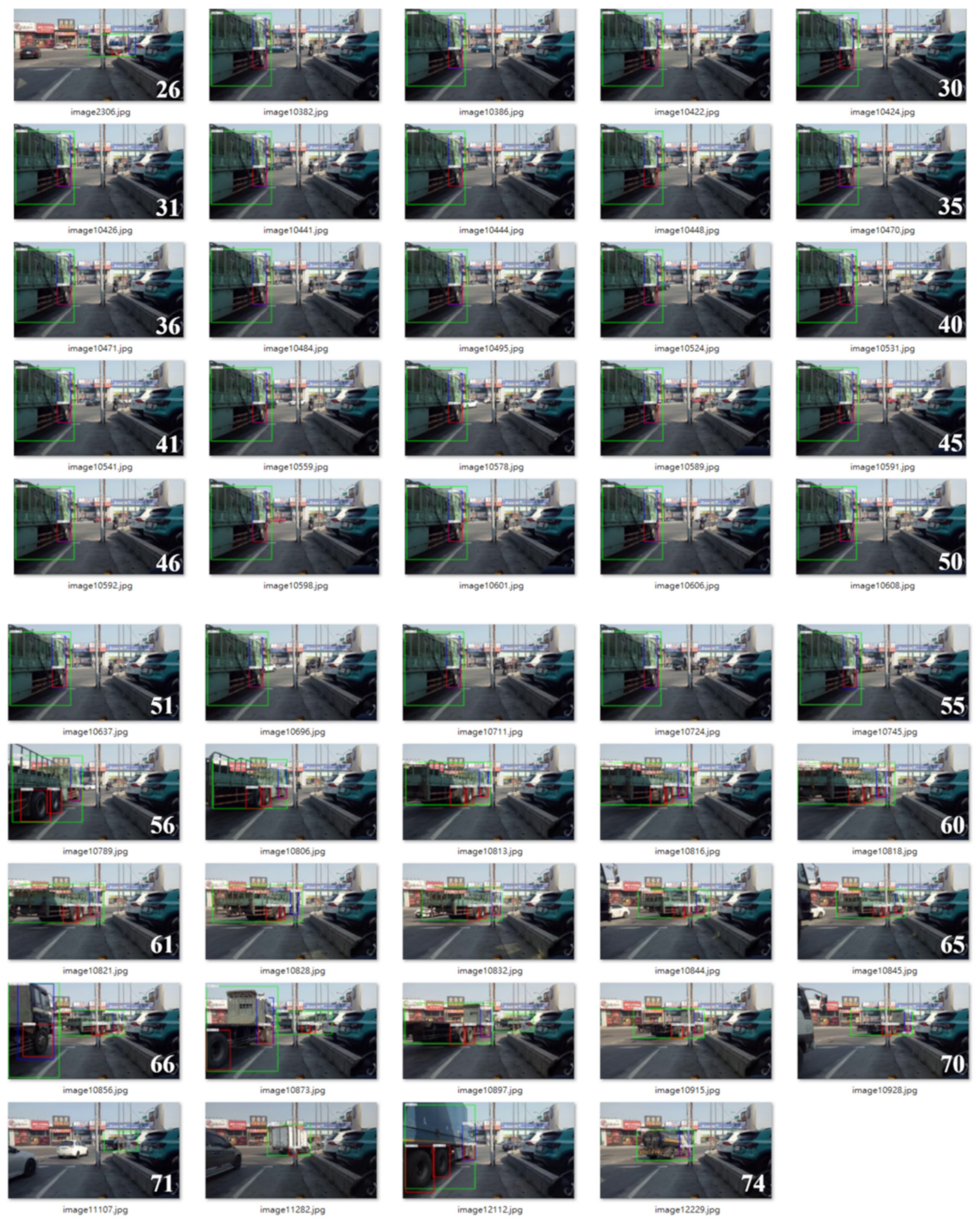
Figure 22. Test image (26~74).

Figure 23. Training curve of Bi-LSTM 10-10.

As in Figure 21, image number sheet 16 to 25, the wheel error detection condition occurs, perhaps after the image compression is not detected in the model features of the wheel; as in Figure 22, the image number sheet 31 to 33 are not marked in the front due to the detection of features similar to the wheel; however, this object is not detected. The car body is detected for several reasons. The image features are not detected by the model because of the size of the object on the image, the color of the object being too similar, and it being obscured by other objects.

Training Results of Cyclic Neural Network Prediction Model

This paper uses a cyclic neural network prediction model to predict the movement trajectory of large vehicles at the intersection. The trajectory data of the trajectory data is to be detected using the object detection model trained in this study. Data analysis and preprocessing delete it or fill the wrong track. This paper compares the LSTM model, Bi-LSTM and Stacked Bi-LSTM model of the architecture of the stacked cyclic neural network architecture, and it will be compared with different input dimensions. The number of layers, different predicted time lengths and different preprocessing methods of data are trained.

This study’s training parameters, such as the cyclic neural network model setting table in Table 5, compare the above two models in four different modes, and then compare them with different preprocessing methods. In terms of training materials, the video taken at the intersection was sampled at 10 Hz, the sample image was sent to the object detection model to capture the trajectory of a large car at the junction, and 312 strokes were taken from the trajectory data as a result of the trajectory data. The test set of training and the results of the training are described below.

Table 5. Cyclic neural network model setup table.

Name	Parameter Value
Input dimension	Two-dimensional or four-dimensional
Predicted length	10 trajectories after 10 trajectory prediction 10 trajectories after 20 trajectory prediction
Maximum number of training steps	12,000
Number of trainings	A total of 312
Number of tests	A total of 31

We set the number of trajectory prediction pens to predict the movement trajectory of the next second (10-10) in one second and two seconds in one second (10-20). The last trained model accuracy (accuracy) is recorded when the trajectory prediction models are trained. In this paper, three different architectures of LSTM models are trained in two different conditions and the results are compared, as shown in the LSTM model comparison table in Table 6.

Table 6. Comparison of training results of LSTM models.

Items	Training Model	Input Data Dimension	Number of Predictions (N-M) (N Data Predictions M Data)	Number of Generations	Accuracy
1	Stacked LSTM	4-Dimension (fx, fy, wx, wy)	10-10	12,000	52.30%
2	Stacked LSTM	4-Dimension (fx, fy, wx, wy)	10-20	12,000	49.30%
3	Stacked LSTM	2-dimensional (x, y)	10-10	12,000	86.43%
4	Stacked LSTM	2-dimensional (x, y)	10-20	12,000	71.75%
5	Bi-LSTM	4-Dimension (fx, fy, wx, wy)	10-10	12,000	62.17%
6	Bi-LSTM	4-Dimension (fx, fy, wx, wy)	10-20	12,000	59.81%
7	Bi-LSTM	2-dimensional (x, y)	10-10	12,000	87.57%
8	Bi-LSTM	2-dimensional (x, y)	10-20	12,000	68.85%
9	Stacked Bi-LSTM	4-Dimension (fx, fy, wx, wy)	10-10	12,000	76.03%
10	Stacked Bi-LSTM	4-Dimension (fx, fy, wx, wy)	10-20	12,000	61.12%
11	Stacked Bi-LSTM	2-dimensional (x, y)	10-10	12,000	87.77%
12	Stacked Bi-LSTM	2-dimensional (x, y)	10-20	12,000	75.29%

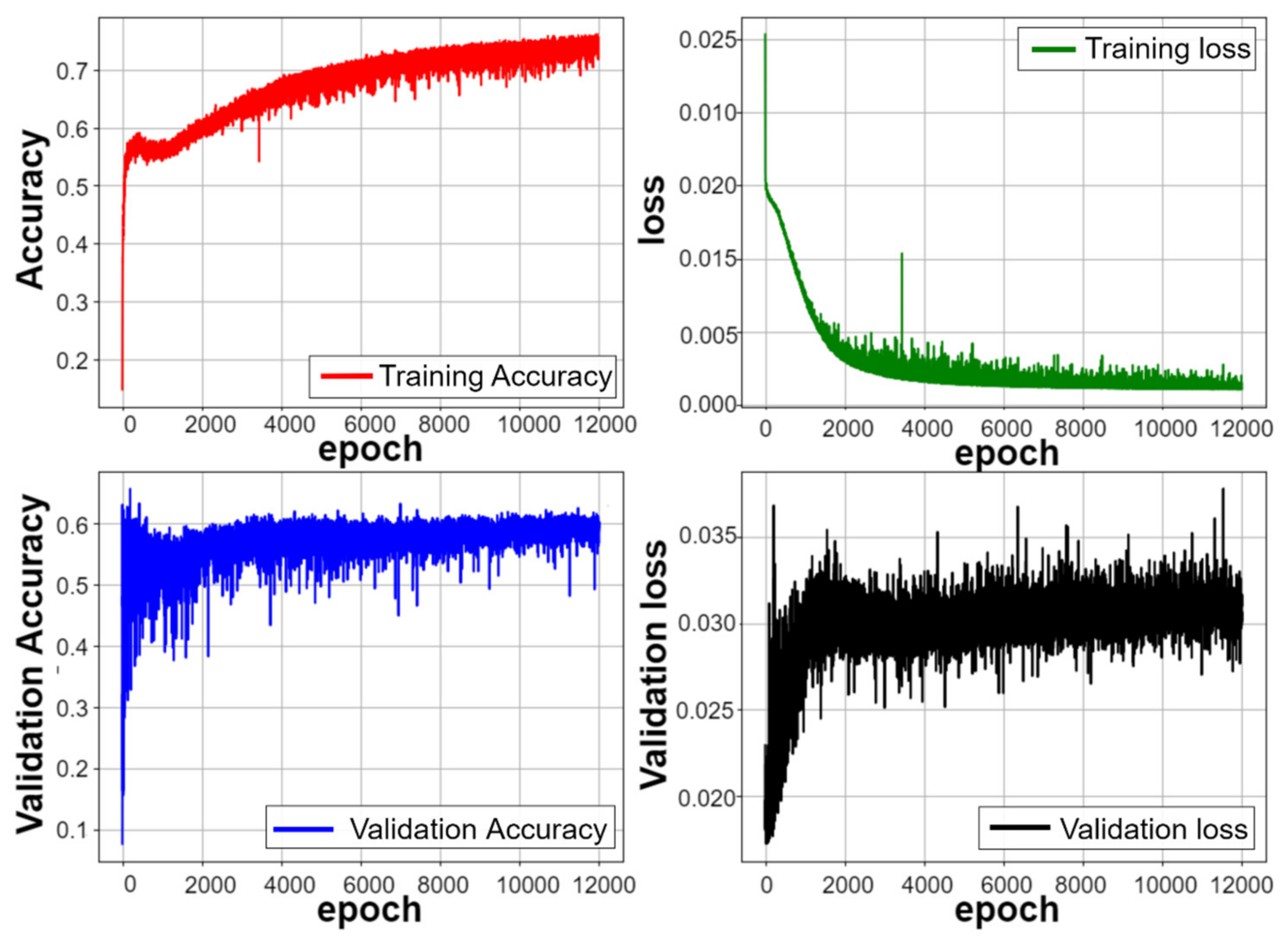
The trajectory prediction model training process is shown in Figure 23 and Figure 24. When training steps are about 2000 steps, the accuracy curve continues to grow and is inversely proportional to the loss curve, indicating that the training is good, no overfitting occurs, and the model begins to smooth when the training steps are close to 4000 steps. The model nears saturation at about 10,000 steps, the total number of steps is set to 12,000 and the overall model training time is about 13 h. It can be found by two training curves and that when predicted with the same number of data pens, the predictive precision of the model is reduced when the prediction time series is extended.

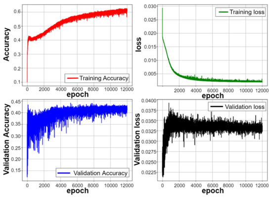
Figure 24. Training curve of Bi-LSTM 10-20.

From Table 6, one can compare input dimensions in different models with forecast lengths and visualize the table section, as shown in Figure 25. It is obvious that the model accuracy of the Stacked Bi-LSTM is generally higher than other models when the re-input dimension is four dimensions (front and rear wheel coordinates). In addition, different prediction lengths have a certain degree of influence on the model and the trajectory prediction. The model accuracy of 10 trajectories after 10 trajectory prediction can be observed in Figure 25 It is higher and the predictive accuracy of Stacked Bi-LSTM is higher than in the other two models at the same input dimension and predicted length.

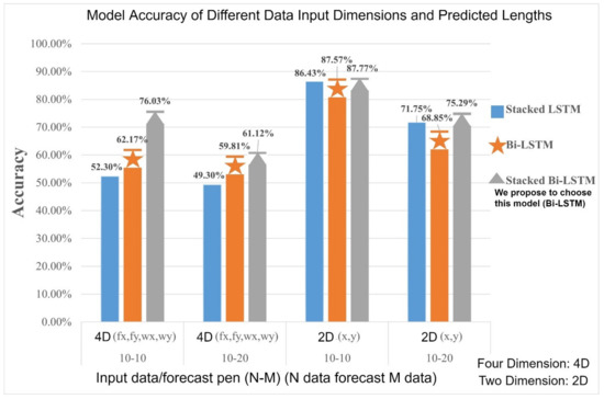
Figure 25. Model accuracy comparison of different data input dimensions and predicted length.

In Figure 25, the accuracy of the longitudinal axis of the chart indicates that the three models (stacked LSTM, Bi LSTM and Bi LSTM stacked) are used under the same setting of this study, as the training set accuracy of the training results. We can find the difference in accuracy between the method used in this paper and other different methods.

This paper uses the following three formulas for the paper review model error tool: Equation (14) is the mean absolute deviation (MAD), Equation (15) is the mean squared error (MSE), and Equation (16) is the mean absolute percentage error (MAPE).

$$\mathrm{MAD}=\frac{\sum \left|{\mathrm{Actual} \mathrm{value}}_t-{\mathrm{Predicted} \mathrm{values}}_t\right|}{n}$$

(14)

$$\mathrm{MSE}=\frac{\sum {\left({\mathrm{Actual} \mathrm{value}}_t-{\mathrm{Predicted} \mathrm{values}}_t\right)}^2}{n-1}$$

(15)

$$\mathrm{MAPE}=\frac{\sum \frac{\left|{\mathrm{Actual} \mathrm{value}}_t-{\mathrm{Predicted} \mathrm{values}}_t\right|}{{\mathrm{Actual} \mathrm{value}}_t}\times 100}{n}$$

(16)

After the trajectory prediction model training is completed, the movement trajectory of 25 groups of large car front or rear wheels that are not put into the model training is the prediction. There is a total of 10-20 ways to predict by recording the average error of each group in order to make a comparison. The comparison results are shown in the Table 7 LSTM model trajectory prediction error comparison table.

Table 7. Trajectory prediction error comparison table for LSTM model.

Items	Training Model	Number of Predictions (N-M) (N Data Predictions M Data)	MAD	MSE	MAPE
1	Stacked LSTM	10-10	27.5799	756.8014	5.5205
2	Stacked LSTM	10-20	32.6421	1103.1558	6.0711
3	Bi-LSTM	10-10	23.3785	493.8061	4.7476
4	Bi-LSTM	10-20	40.0393	1593.683	7.6167
5	Stacked Bi-LSTM	10-10	14.4397	242	3.0556
6	Stacked Bi-LSTM	10-20	22.3255	643	4.3622

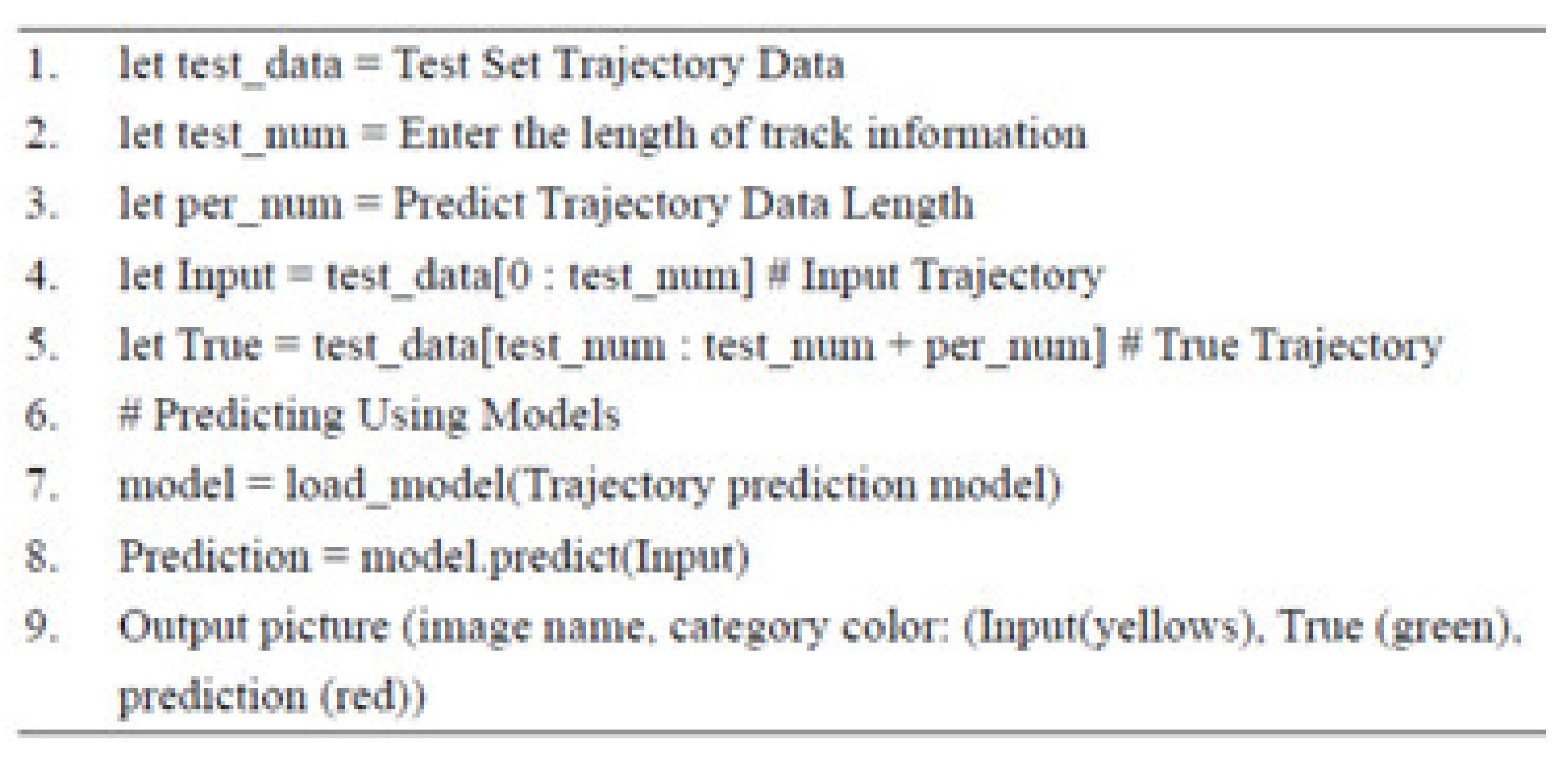
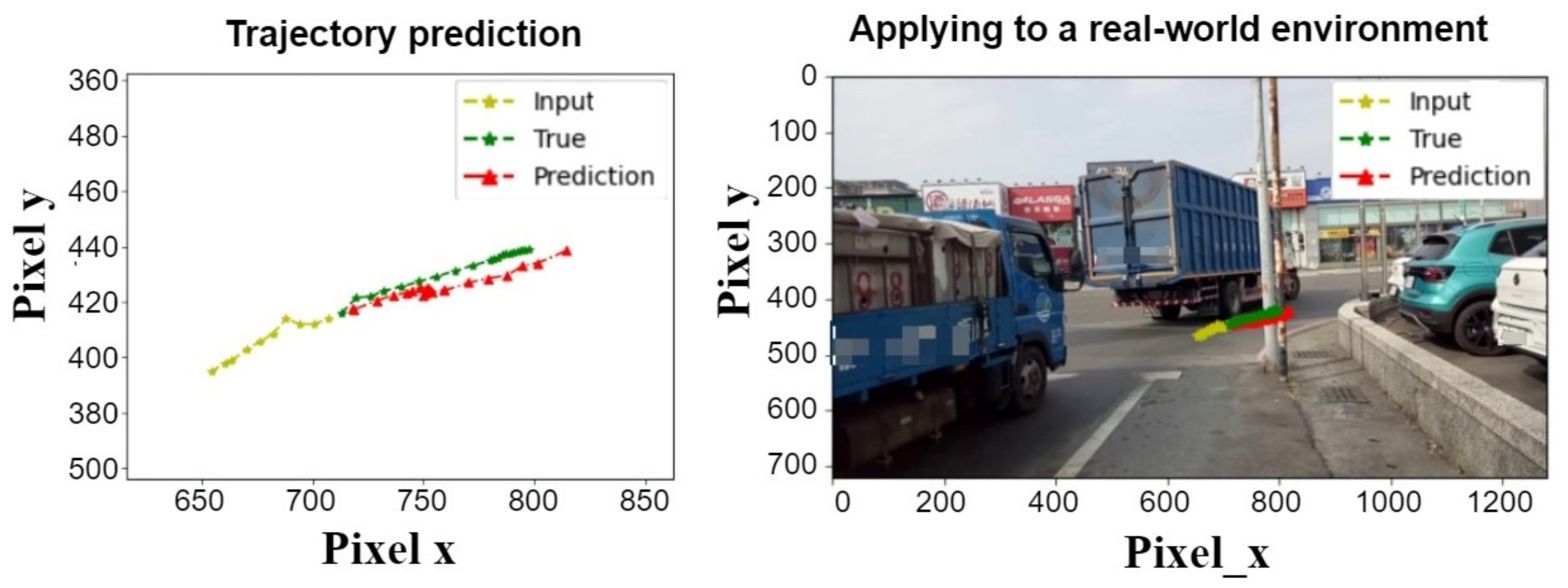
The trajectory prediction results output the pseudocode in Figure 26, split the test set data according to the predicted length of the trajectory model, split it into input and real trajectory, and put the input trajectory into the trajectory prediction model, Predict, and finally, compare the predicted trajectory to the real track output chart. Figure 27 shows the bi-LSTM trajectory prediction control graph. The next two seconds (20 trajectories) are predicted in one second (10 trajectories). The left is the result of the trajectory prediction, and on the right, the predicted trajectory is on the actual image, with yellow lines representing the previous second input. The red represents the last two seconds of the model’s predicted trajectory, and the green represents the true trajectory of the next two seconds.

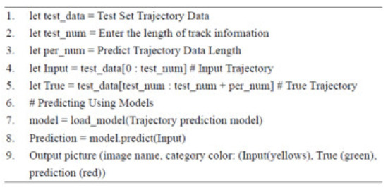
Figure 26. Trajectory prediction result output pseudocode (#: indicates a comment).

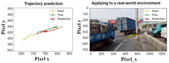
Figure 27. Bi-LSTM trajectory prediction.

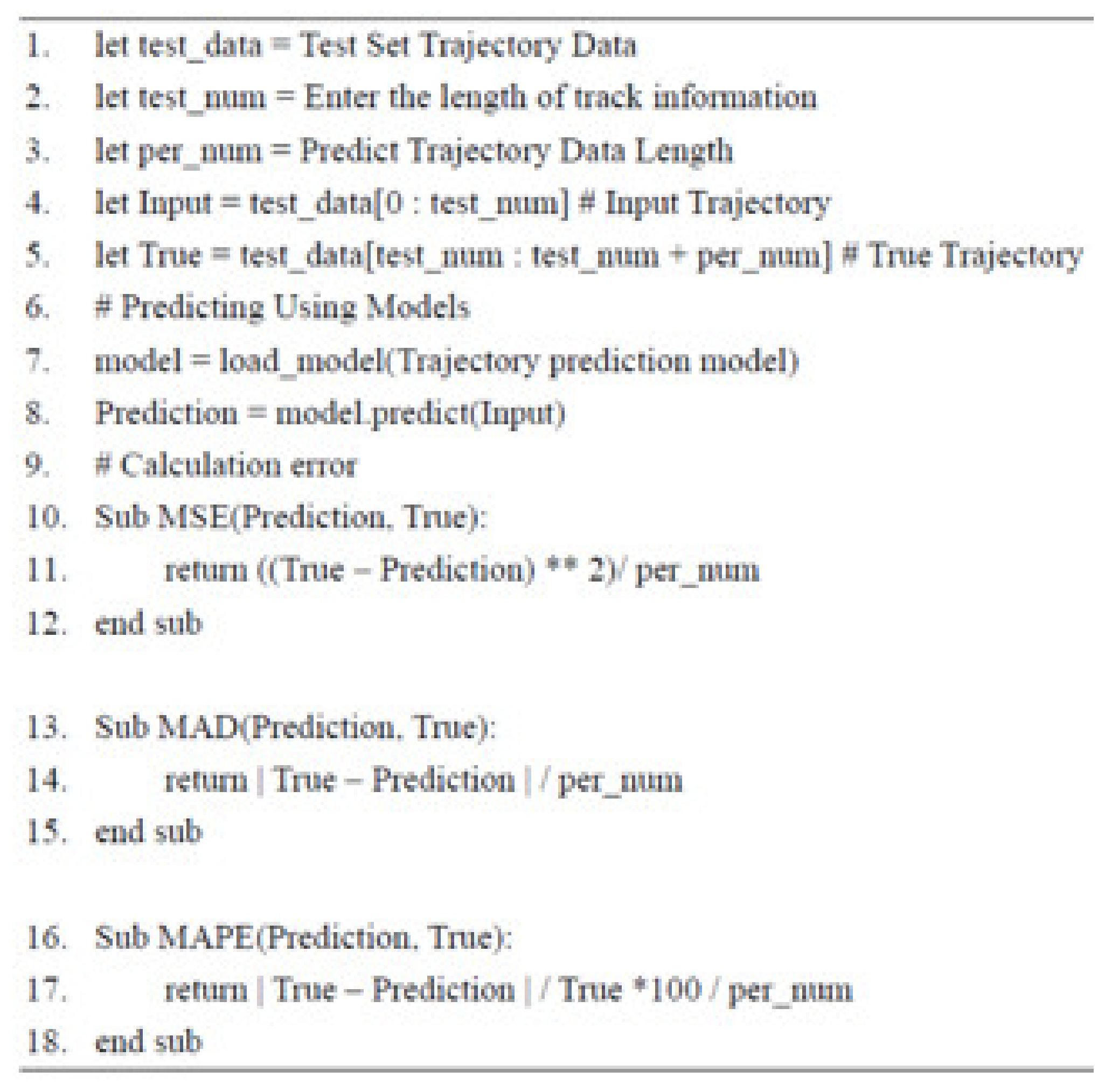
Figure 28 evaluates the prediction model error pseudocode. It calculates and outputs the predicted and true trajectory into the letter, and calculates and outputs the predicted absolute deviation, mean square error and average absolute percentage error, and records the results into the trajectory of the Table 7 LSTM model forecast error comparison table. One can compare the predictive results for each LSTM model to evaluate the predictive accuracy of the model in a mean absolute deviation, mean square error and average absolute percentage error, and the results are plots in long bars as a way to compare.

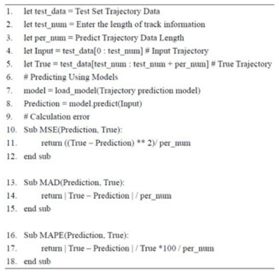
Figure 28. Evaluating prediction model error pseudocode (#: indicates a comment).

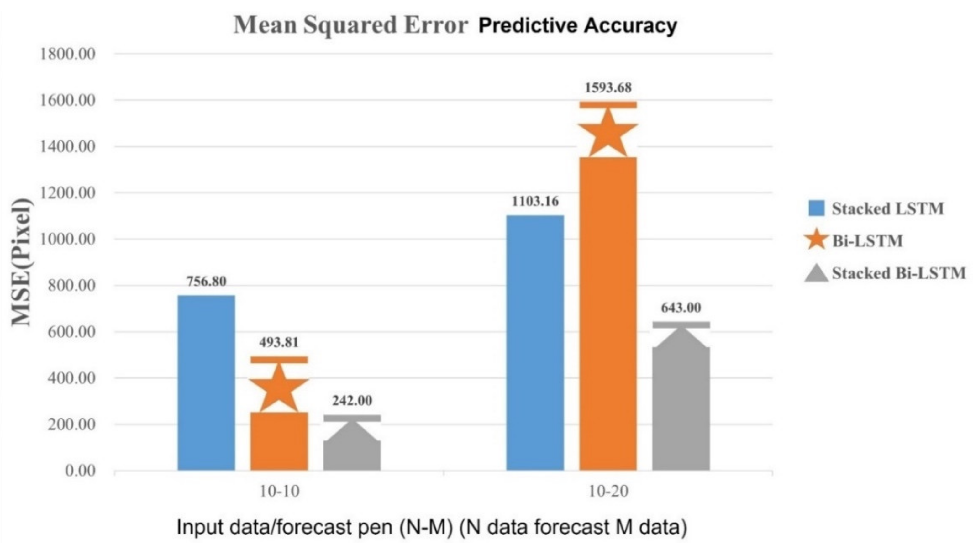
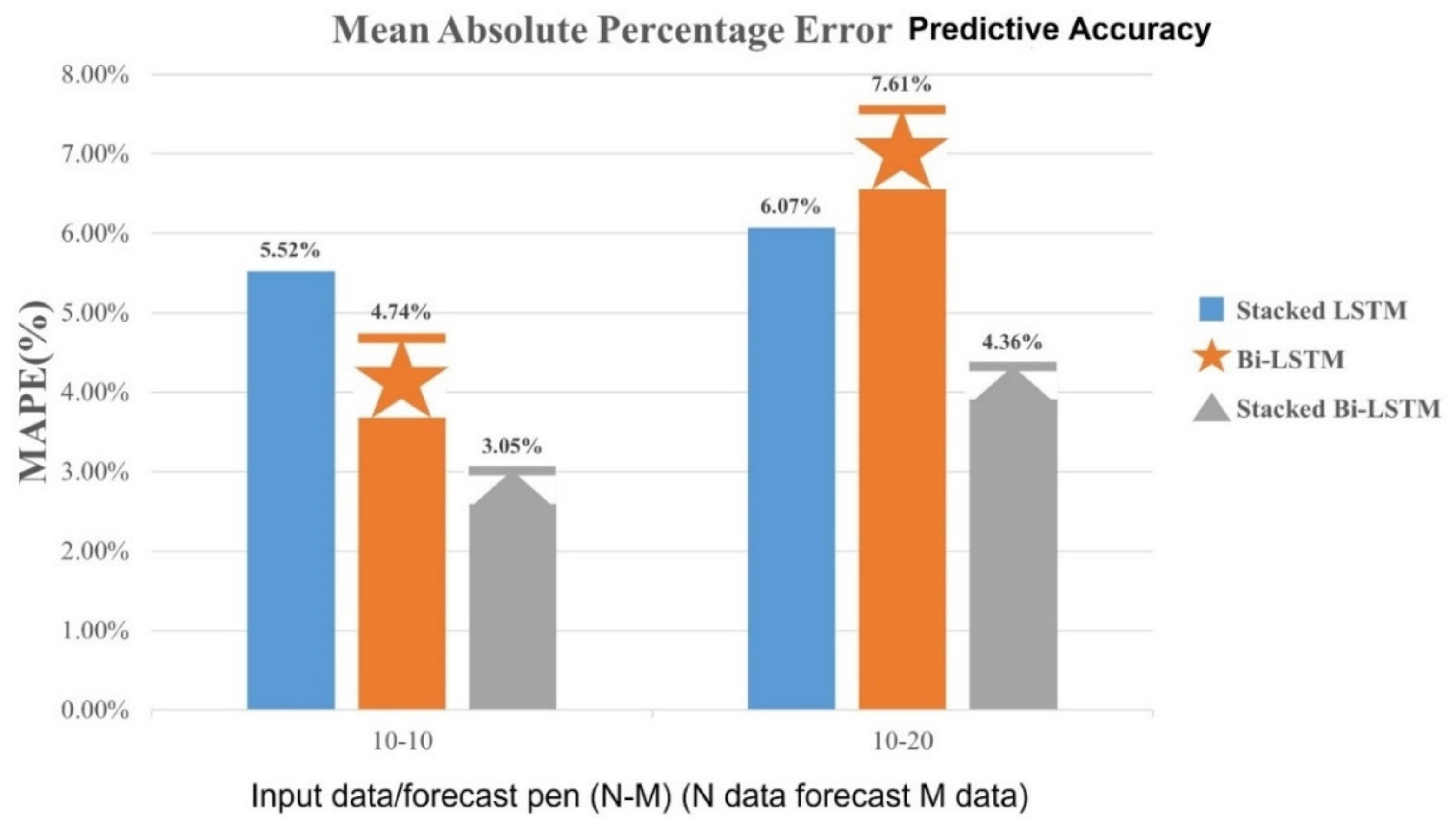
As shown in Figure 29, Figure 30 and Figure 31, the error of Stacked Bi-LSTM in prediction is generally lower than other LSTM models. It was found that the single-layer Bi-LSTM model predicts longer time-series data, the error is higher than the stacked Stacked LSTM model. Based on the above numerical results of the MAD average absolute deviation, MSE mean square error and MAPE average absolute percentage error, the Stacked Bi-LSTM is better at predicting the moving trajectory then the other two LSTM model architectures.

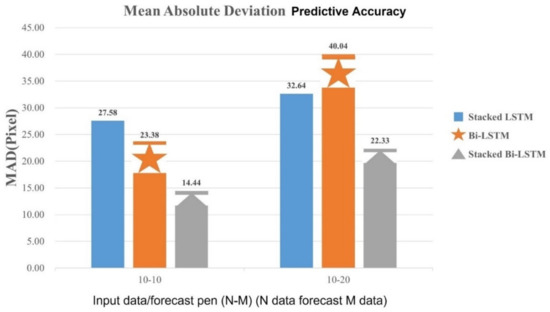
Figure 29. Predictive accuracy comparison of three models using MAD.

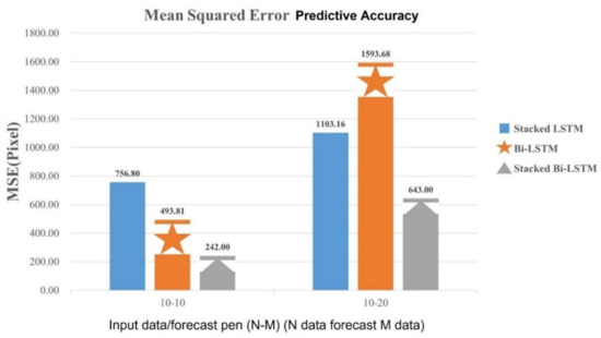
Figure 30. Comparison of three models using MSE prediction accuracy.

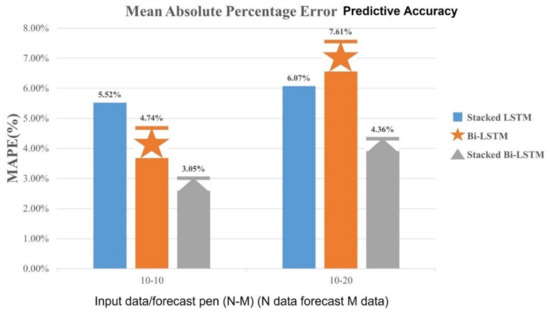
Figure 31. Comparison of three models using MAPE prediction accuracy.

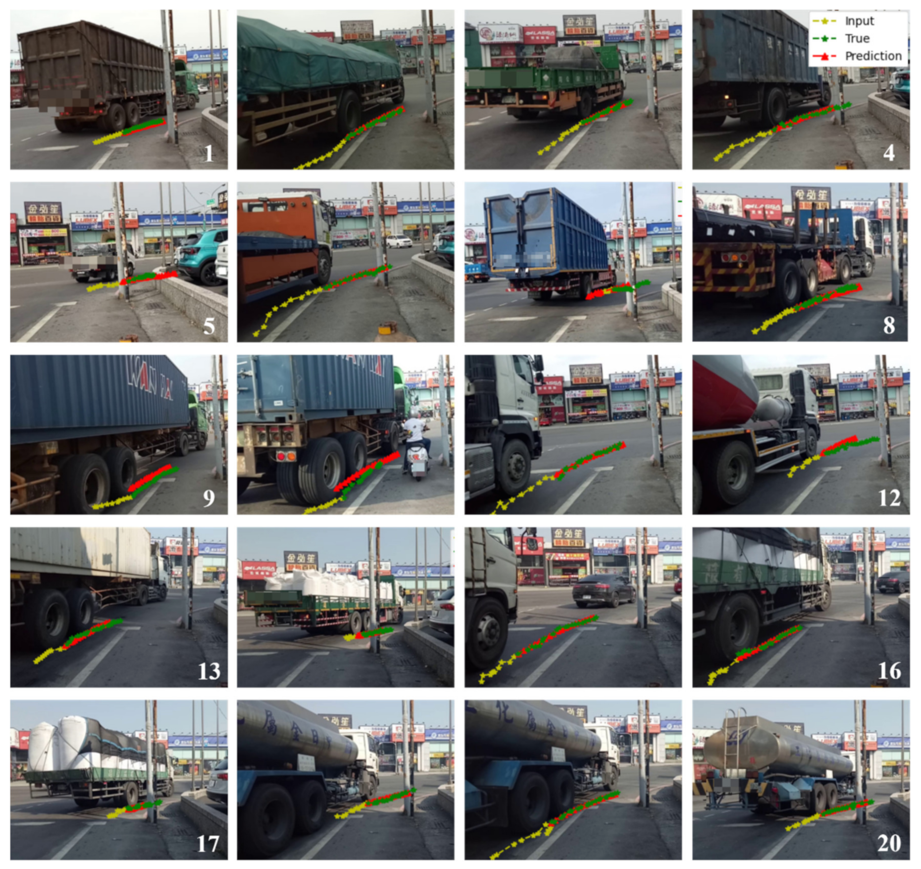
As shown in Figure 32, the trajectory prediction test image (1~20) of the trajectory prediction model training is completed, and 20 sets of trajectory data from untrained trajectory data will be selected into the model. The Stacked Bi-LSTM model predicts 10–20 trajectory data, and the yellow means the input will first put a second moving trajectory (10 strokes) into the model. The red represents the prediction, and the green represents the true movement trajectory (true) in the track data and presents the data on the real image. The predicted trajectory is basically similar to the real trajectory, but there is an error in some of the predictions.

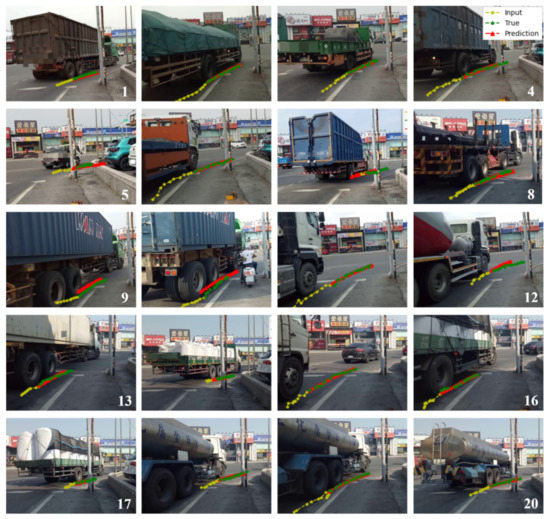
Figure 32. Trajectory prediction test image (1~20).

5. Conclusions

The contribution of this paper is to predict the inner wheel path trajectory of large cars from the perspective of the locomotive knight through object detection models and cyclic neural network models, and with image recognition through deep learning. The images are collected and analyzed to predict possible hazards by predicting the trajectory of the movement of large wheels.

This paper predicts the turning trajectory of large vehicles at the intersection by using object detection algorithms and cyclic neural network models; we analyzed object detection models such as YOLOv3, YOLOv4, Faster RCNN, MobileNet ver2 SSD and YOLOv4 models, which have a 95% average accuracy compared to other models with high precision. This paper looks for a trajectory prediction model using Stacked Bi-LSTM and proposes an 87.77% prediction accuracy when predicting subsequent trajectories with one-second trajectory data, and a 75.75% accuracy for two-second trajectory data. The Stacked Bi-LSTM model predicted error is also lower in terms of prediction errors versus the other two models.

This paper is made by stacking various basic technologies, and there are many improvements in the research. In future works, the category of object detection and capture will be added, and more vehicle features will be added, so that the vehicle type can still be judged when the vehicle is obscured, improving the accuracy and speed of object detection and object tracking, and using the object detection method to automatically mark and segment the video trajectory data. In terms of trajectory prediction, more large-scale wheel trajectory data are added, and road environmental parameters and weather factors are added to the model. Batch normalization and regularization methods are added to the model to reduce the problem of overfitting when training the model. We hope that through these improvements, the whole system can operate more smoothly. The system is integrated into the motorcycle to make the motorcycle driving perspective predict the wheel trajectory in the large car and warn the driver, so as to reduce the probability of accidents with large cars.

References

- World Health Organization. Global Status Report on Road Safety 2018: Summary; World Health Organization: Geneva, Switzerland, 2018.
- Caliendo, C.; De Guglielmo, M.L.; Guida, M. Comparison and analysis of road tunnel traffic accident frequencies and rates using random-parameter models. J. Transp. Saf. Secur. 2016, 8, 177–195. [Google Scholar] [CrossRef]
- Wu, Y.; Abdel-Aty, M.; Lee, J. Crash risk analysis during fog conditions using real-time traffic data. Accid. Anal. Prev. 2018, 114, 4–11. [Google Scholar] [CrossRef] [PubMed]
- Kopelias, P.; Papadimitriou, F.; Papandreou, K.; Prevedouros, P. Urban freeway crash analysis: Geometric, operational, and weather effects on crash number and severity. Transp. Res. Rec. 2015, 9, 123–131. [Google Scholar] [CrossRef]
- Sharma, K.P.; Poonia, R.C.; Sunda, S. Accurate real-time location map matching algorithm for large scale trajectory data. In Proceedings of the 2018 7th International Conference on Reliability, Infocom Technologies and Optimization (Trends and Future Directions) (ICRITO), Noida, India, 29–31 August 2018; pp. 646–651. [Google Scholar] [CrossRef]
- Chen, Q.H.; Huang, H.; Li, Y.; Lee, J.; Long, K.J.; Gu, R.; Zhai, X. Modeling accident risks in different lane-changing behavioral patterns. Anal. Methods Accid. Res. 2021, 30, 100159. [Google Scholar] [CrossRef]
- Road Traffic Safety Committee. Road Traffic Accident (within 30 Days)—According to the Type of Driving by the First Party. Available online: https://stat.motc.gov.tw/mocdb/stmain.jsp?sys=220&ym=10501&ymt=10912&kind=21&type=1&funid=b330704&cycle=41&outmode=0&compmode=0&outkind=1&fldlst=111&codspc0=0,2,4,1,&rdm=pqbiczld (accessed on 10 August 2021).
- Park, S.H.; Kim, B.; Kang, C.M.; Chung, C.C.; Choi, J.W. Sequence-to-sequence prediction of vehicle trajectory via lstm encoder-decoder architecture. In 2018 IEEE Intelligent Vehicles Symposium (IV); IEEE: Changshu, China, 2018; pp. 1672–1678. [Google Scholar]
- Altché, F.; de La Fortelle, A. An lstm network for highway trajectory prediction. In Proceedings of the 2017 IEEE 20th International Conference on Intelligent Transportation Systems (ITSC), Yokohama, Japan, 16–19 October 2017; pp. 353–359. [Google Scholar]
- Xue, H.; Huynh, D.Q.; Reynolds, M. Bi-Prediction: Pedestrian trajectory prediction based on bidirectional LSTM classification. In Proceedings of the 2017 International Conference on Digital Image Computing: Techniques and Applications (DICTA), Sydney, NSW, Australia, 29 November–1 December 2017; pp. 1–8. [Google Scholar] [CrossRef]
- Xia, C.; Weng, C.Y.; Zhang, Y.; Chen, I.M. Vision-based measurement and prediction of object trajectory for robotic manipulation in dynamic and uncertain scenarios. IEEE Trans. Instrum. Meas. 2020, 69, 8939–8952. [Google Scholar] [CrossRef]
- Ip, A.; Irio, L.; Oliveira, R. Vehicle trajectory prediction based on LSTM recurrent neural networks. In Proceedings of the 2021 IEEE 93rd Vehicular Technology Conference (VTC2021-Spring), Helsinki, Finland, 25–28 April 2021; pp. 1–5. [Google Scholar]
- Howard, A.G.; Zhu, M.; Chen, B.; Kalenichenko, D.; Wang, W.; Weyand, T.; Andreetto, M.; Adam, H. MobileNets: Efficient Convolutional Neural Networks for Mobile Vision Applications. arXiv 2017, arXiv:1704.04861. [Google Scholar]
- Sandler, M.; Howard, A.; Zhu, M.; Zhmoginov, A.; Chen, L.C. MobileNetV2: Inverted residuals and linear bottlenecks. In Proceedings of the 2018 IEEE/CVF Conference on Computer Vision and Pattern Recognition, Salt Lake City, UT, USA, 18–21 June 2018; pp. 4510–4520. [Google Scholar]
- Redmon, J.; Divvala, S.; Girshick, R.; Farhadi, A. You only look once: Unified, real-time object detection. In Proceedings of the 2016 IEEE Conference on Computer Vision and Pattern Recognition (CVPR), Las Vegas, NV, USA, 27–30 June 2016; pp. 779–788. [Google Scholar]
- Redmon, J.; Farhadi, A. YOLO9000: Better, faster, stronger. In Proceedings of the 2017 IEEE Conference on Computer Vision and Pattern Recognition (CVPR), Honolulu, HI, USA, 21–26 July 2017; pp. 6517–6525. [Google Scholar]
- Redmon, J.; Farhadi, A. YOLOv3: An Incremental Improvement. arXiv 2018, arXiv:180402767. [Google Scholar]
- Lin, T.-Y.; Dollr, P.; Girshick, R.; He, K.; Hariharan, B.; Belongie, S. Feature pyramid networks for object detection. In Proceedings of the 2017 IEEE Conference on Computer Vision and Pattern Recognition (CVPR), Honolulu, HI, USA, 21–26 July 2017; pp. 936–944. [Google Scholar]
- Bochkovskiy, A.; Wang, C.-Y.; Liao, H. YOLOv4: Optimal speed and accuracy of object detection. In Proceedings of the Computer Vision and Pattern Recognition, Seattle, WA, USA, 13–19 June 2020. [Google Scholar]
- Ren, S.; He, K.; Girshick, R.; Sun, J. Faster R-CNN: Towards Real-Time Object Detection with Region Proposal Networks. Adv. Neural Inf. Process. Syst. 2015, 28, 91–99. [Google Scholar] [CrossRef] [PubMed] [Green Version]
- Girshick, R.; Donahue, J.; Darrell, T.; Malik, J. Rich Feature hierarchies for accurate object detection and semantic segmentation. In Proceedings of the 2014 IEEE Conference on Computer Vision and Pattern Recognition, Columbus, OH, USA, 23–28 June 2014; pp. 580–587. [Google Scholar]
- Girshick, R. Fast R-CNN. In Proceedings of the 2015 IEEE International Conference on Computer Vision (ICCV), Santiago, Chile, 7–13 December 2015; pp. 1440–1448. [Google Scholar]
- Liu, W.; Anguelov, D.; Erhan, D.; Szegedy, C.; Reed, S.; Fu, C.Y.; Berg, A.C. SSD: Single Shot MultiBox Detector. arXiv 2016, arXiv:1512023259905, 21–37. [Google Scholar]
- Kitani, K.M.; Ziebart, B.D.; Bagnell, J.A.; Hebert, M. Activity forecasting. In Proceedings of the European Conference on Computer Vision (ECCV), Florence, Italy, 7–13 October 2012; pp. 201–214. [Google Scholar]
- Finn, C.; Goodfellow, I.; Levine, S. Unsupervised Learning for Physical Interaction through Video Prediction. Adv. Neural Inf. Processing Syst. 2016, 29, pp.64–72. [Google Scholar]
- Lotter, W.; Kreiman, G.; Cox, D. Deep Predictive Coding Networks for Video Prediction and Unsupervised Learning. arXiv 2016, arXiv:1605.08104. [Google Scholar]
- Luc, P.; Neverova, N.; Couprie, C.; Verbeek, J.; LeCun, Y. Predicting Deeper into the Future of Semantic Segmentation. arXiv 2017, arXiv:170307684. [Google Scholar]
- Huang, S.; Li, X.; Zhang, Z.; He, Z.; Wu, F.; Liu, W.; Tang, J. Deep Learning Driven Visual Path Prediction from a Single Image. IEEE Trans. Image Process. 2016, 25, 5892–5904. [Google Scholar] [CrossRef] [PubMed] [Green Version]
- Kim, B.; Kang, C.M.; Kim, J.; Lee, S.H.; Chung, C.C.; Choi, J.W. Probabilistic Vehicle Trajectory Prediction over Occupancy Grid Map via Recurrent Neural Network. arXiv 2017, arXiv:170407049. [Google Scholar]
- Xing, Y.; Lv, C.; Cao, D. Personalized Vehicle Trajectory Prediction Based on Joint Time-Series Modeling for Connected Vehicles. IEEE Trans. Veh. Technol. 2020, 69, 1341–1352. [Google Scholar] [CrossRef]
- Bandara, K.; Bergmeir, C.; Hewamalage, H. LSTM-MSNet: Leveraging Forecasts on Sets of Related Time Series With Multiple Seasonal Patterns. IEEE Trans. Neural Netw. Learn. Syst. 2021, 32, 1586–1599. [Google Scholar] [CrossRef] [PubMed] [Green Version]
- Hochreiter, S.; Schmidhuber, J. Long Short-Term Memory. Neural Comput. 1997, 9, 1735–1780. [Google Scholar] [CrossRef] [PubMed]
- Schuster, M.; Paliwal, K. Bidirectional recurrent neural networks. Signal Process. IEEE Trans. 1997, 45, 2673–2681. [Google Scholar] [CrossRef] [Green Version]
- Tzutalin. Labelimg. GitHub. Available online: https://github.com/tzutalin/labelImg (accessed on 10 August 2021).
Publisher’s Note: MDPI stays neutral with regard to jurisdictional claims in published maps and institutional affiliations. |
© 2022 by the authors. Licensee MDPI, Basel, Switzerland. This article is an open access article distributed under the terms and conditions of the Creative Commons Attribution (CC BY) license (https://creativecommons.org/licenses/by/4.0/).