Article

A Temporal Perspective in Eco2 Building Design

by
Patricia Schneider-Marin
1,2,* and
Werner Lang
1
1
Institute of Energy Efficient and Sustainable Design and Building, TUM School of Engineering and Design, Technical University of Munich (TUM), Arcisstr. 21, 80333 Munich, Germany
2
Department of Architecture and Technology, Faculty of Architecture and Design, Norwegian University of Science and Technology (NTNU), Alfred Getz’ vei 3, 7491 Trondheim, Norway
*
Author to whom correspondence should be addressed.
Sustainability 2022, 14(10), 6025; https://doi.org/10.3390/su14106025
Submission received: 6 April 2022 / Revised: 7 May 2022 / Accepted: 9 May 2022 / Published: 16 May 2022
(This article belongs to the Special Issue Life Cycle Thinking and Sustainability Assessment of Buildings)

Abstract

:
The architecture, engineering and construction (AEC) sector has great potential and responsibility for reducing its considerable resource consumption and high share of global emissions. However, economic factors are often cited as barriers to more environmentally friendly solutions in building design. Hence, environmental and economic life cycle assessment (LCA and LCC) are of utmost importance in building design. They serve as the base methodologies for what we call the “Eco2” framework. In this context, monetary valuation of multiple environmental impacts allows to integrate the results as a basis for design decisions. A case study representative of small-scale office buildings in Germany illustrates the Eco2 framework and shows the influence of temporal parameters (discount rates and price changes), as well as of differing monetary valuation, on the ranking of design options. Varying the temporal parameters affects the ranking of different solutions for the structure and finishes of the case study building but not for its mechanical, electrical and plumbing (MEP) systems and operation. However, the ratio of environmental life cycle cost (eLCC) to financial life cycle cost (fLCC) is significantly higher for MEP systems and operation than for the structure and finishes. This investigation shows that it is possible to achieve simultaneous emission and cost savings, whereas temporal factors can decisively influence decision making in design processes.

1. Introduction

Demand for comfortable indoor environments is growing globally, but the architecture, engineering and construction (AEC) sector is already responsible for 37% of global GHG (greenhouse gas) emissions [1] and consumes a large share of Europe’s material resources, especially minerals and metals [2]. The sector is falling short of reducing emissions and resource consumption [3] while trying to meet global demand. Frequently, economic barriers are cited as a reason for the slow change in the AEC sector [4]. Hence, to speed up the transition, it is not sufficient to calculate emissions for different building solutions, disregarding economic factors, or vice versa.
Additionally, a long-term life cycle view urgently needs to replace the prevalent short-time perspective in building design. This entails considering life cycle costs rather than investment costs only and life cycle emissions rather than emissions caused by operational energy use only, the latter being in the focus of current building regulation [5]. For both perspectives, life cycle methods have been established: life cycle assessment (LCA) for the emissions perspective and life cycle costing (LCC) for economic calculations. Integrating both into design processes offers the opportunity to identify win–win situations and to indicate economically viable emissions savings to building clients and stakeholders. From a policy perspective, solutions with high emissions saving potential, which are currently economically unattractive, can be supported, e.g., by financial incentives.
Work on both LCA [6] and LCC [7] in green building design, as well as on a parallel use of both [8], has increased considerably in the past decade, but there are still methodological gaps for an integrated use, and neither method is part of standard building design processes. Therefore, we developed what we call the “Eco2” (ecology × economy = Eco2) framework [9] for an integrated use of LCA and LCC in building design. This framework uses a common life cycle inventory for LCA and LCC, mapping environmental and economic data to it, as well as common data, such as reference service lives (RSLs). For result integration, monetary valuation of impacts is used. Here, we illustrate and test the framework with a case study. The case study was selected to fill information gaps in previous studies by including mechanical, electrical and plumbing (MEP) systems in both LCA and LCC calculations and their respective embedded and operational impacts. Additionally, we developed a limited database for this case study to allow for the combination of differing building subsystems. Previous studies have tended to consider either tradeoffs between embedded and operational emissions and cost [10] or optimization of envelope energy systems and emissions [11], disregarding embedded emissions in energy systems, although in a real design process, all aspects need to be taken into account.
As operational energy use has been identified as one of the major causes of GHG emissions while bearing the most economically favorable emissions savings, the EU established ecodesign regulations for some energy-consuming appliances (e.g., heating and cooling appliances) [12] but neither for buildings nor for building products. Ecodesign specifically targets financial savings by redesigning products for emissions saving and has proven that savings potential is considerable.
Using monetary valuation for result integration has only been tested in a few studies [13,14] but bears the opportunity to juxtapose environmental and economic goals. An integrated use of LCA and LCC whilst valuing emissions in monetary terms enables transfer of the quasi-dynamic approach from LCC to LCA, thereby considering identical scenarios for both environment and economics. Fully dynamic LCA and LCC require dynamic inventories, as well as the inclusion of uncertainties in future developments, such as the marginal effect of emissions [15]. Dynamic inventories for LCA consider changes in energy supply [16] and/or the increase in production efficiency [17], whereas for LCC, such inventories should include material-specific criticality. A quasi-dynamic approach simplifies this process by introducing gradual annual changes. Their effect is exponential and allows for variant studies testing different scenarios. Adding temporal parameters into LCA has not previously been implemented in simultaneous building LCA + LCC evaluations. Therefore, we aim to test the influence of discounting and price change assumptions, as well as the use of differing monetary values for emissions, on the comparison and resulting ranking of proposed building solutions.
A fully integrated Eco2 approach has the potential to show the value of emissions savings in design processes and identify solutions with low-cost or even profitable emissions saving. Introducing the life cycle perspective shifts the focus from limited investment cost considerations to a wider spectrum of evaluation. As a consequence of the future perspective, temporal factors allow for consideration of uncertainties in the development of the environment and the economy. In this context, the main question of this research is how and to what extent such temporal factors influence decision making in building design.

2. Method: Eco2

Life cycle assessment (LCA) and life cycle costing (LCC) are at the core of the Eco2 framework [9]. We employ this framework, using monetary valuation as a weighting method, to arrive at one value for LCA results, and varying temporal parameters to test their effect on design recommendations.

2.1. Goal and Scope

An office building with a gross floor area of approximately 1200 m2 serves as case study. The FTmehrHAUS has three floors and was built in 2016. The building has a simple rectangular shape with a regular façade and is representative of a standard small office building in Germany [18]. It served as a case study in the Early BIM project [19] for the investigation of opportunities of using semantically rich BIM models in early design phases and in related studies [13,20,21,22,23,24,25] because detailed information about the building has been made available by the owner. Table 1 shows the relevant parameters and boundary conditions for the Eco2 analysis.
The case study looks at the following questions:
  • Which material and energy supply solutions result in the lowest environmental impacts, expressed in environmental life cycle costs (eLCC) and/or the lowest financial life cycle costs (fLCC)?
  • Do temporal parameters change recommendations?
  • Does monetary valuation change recommendations?

2.2. Life Cycle Phases

Currently, no database provides inventory and impact data for calculating environmental and economic impacts in all life cycle phases, and different phases are excluded from LCA or LCC [9]. For instance, life cycle phases A4 (transport gate to site) and A5 (construction) are rarely accounted for in LCA, whereas it is customary that these values are included in the construction prices by default but they are not listed separately. Consequently, C1 (demolition) and C2 (transport site to waste processing or disposal) are included in LCC but disregarded in LCA. For our study, this discrepancy in system boundaries is accepted (Table 1), as previous studies have found that environmental impacts from these phases are comparatively small.
Life cycle phase D (benefits and loads outside of the system boundary) is controversially discussed in the literature [31], as it is outside of the system boundary of the building; hence, benefits from phase D should potentially be accounted for in a different system. On the other hand, phase D contains important information on the circularity potential of buildings. In LCA, recyclable virgin materials that show high impacts in the product stage (A1–A3) receive credits in phase D for avoided impacts (e.g., metals) [32]. Additionally, for materials serving as secondary fuels (e.g., wood and plastics), the offset of emissions against the current energy mix is credited. Materials with a high residual value because of their scarcity or energy-intensive production, such as metals, should also receive financial credits in LCC. However, these credits (e.g., for scrap metal) can be very small compared to investment cost [33], and they happen in the distant future. Moreover, in the databases used for this study, disposal costs include potential material values but do not consider them separately, i.e., if there are economic benefits for phase D, they are merged with the demolition and disposal cost. This is in line with the findings of [4] that the environmental impacts of the end-of-life phase are disproportionally more intensely studied than the economic impacts. For this study, each life cycle phase, including phase D, is calculated separately to allow for the tracking of drivers of impacts.

2.3. Functional Unit

Although both LCA and LCC use a functional unit, which, in principle, facilitates comparability, this is not always specified in studies and can even vary within a sustainability certification system. Specifically, the German building sustainability certification systems DGNB and BNB express LCA results as indicator per m2 NFA (net floor area) per year, where indicators include, among others, GWP and acidification potential (AP) [34,35]. The unit for LCC results, on the other hand, is EUR per m2 GFA (gross floor area) [36,37].

2.4. Building Decomposition

In the German context, the two commonly employed systems for building decomposition were developed for cost calculation and cost monitoring. One system [38] subdivides the building into so-called cost groups (CGs). The second common system, employed primarily in bidding and construction, focuses on trades [39]. It is less apt for environmental (material-focused) evaluation, as, firstly, granularity is too high for design phases with open decisions, and secondly, alternatives are harder to compare, as they are ordered by the trade involved rather than equivalent building parts. CGs are frequently used for disaggregation of the building in LCA [40], as this subdivision is already familiar to designers from cost estimation and calculation. CG 300 (structure and finishes) and CG 400 (MEP systems) are directly related to the building. CGs are applicable to all embedded (material-related) impacts, whereas for impacts caused by operational energy consumption, a separate category, life cycle phase B6, is necessary. However, B6 is closely linked to CG 400, as the type of MEP system has a major influence on emissions in phase B6 [41].

2.5. Scenario Development

For the scenario analysis, the decisive question is whether a change in the parameters, such as discount rates, price increases, or the inclusion of life cycle phase D, changes the ranking of possible solutions. This investigation shows whether the framework influences an environmental–economic recommendation to stakeholders.
Figure 1 shows the construction and energy source variations for the sample project. We aim to cover the majority of standard construction parts and a selection of heating systems. As quantifying the tradeoff between energy standard and embedded emissions is not the primary goal of this study, we excluded the mutual influence of CG 300 and CG 400 + B6. Therefore, we kept the energy standard and the heat/cold distribution constant. For example, all variations of the building contain floor heating. As such, we can consider the variations of CG 300 and CG 400 + B6 separately. For a decision-making process, these subsystems can be optimized separately and recombined to obtain a complete solution.

2.6. Time-Based Life Cycle Inventory

To integrate the two different life cycle approaches, LCA and LCC, it is necessary to use the same bill of quantities for the life cycle inventory and an integrated database for both environmental and economic values with the same base year. Matrices showing the data for each life cycle phase and each building element or material are at the core of the LCI, containing all necessary information for the subsequent impact assessment (Figure 2).

2.7. Impact Assessment

LCA and LCC were calculated in parallel through adata collection specifically created for this study. We limited environmental data for this study to materials and processes contained in Oekobaudat [26]. The life cycle inventory for the environmental calculation was also used for the life cycle cost analysis, i.e., only products and processes available in Oekobaudat were included in cost calculations to avoid differing system boundaries. Cost data were sourced from a commonly used dictionary of construction prices (Baupreislexikon [27]), with a few remaining data gaps filled by BKI [28] and Sirados [29]. Building elements were priced (investment cost and replacement cost), and maintenance and repair costs were tied to specific building elements (e.g., cleaning costs were associated with surfaces). The data source for the latter is the German certification system BNB [37]. End-of-life costs were attached to the specific building material or building part to be exchanged or demolished. These cost values are based on the assumption of careful disassembly and separation of building materials. The available cost data do not allow for differentiation between demolition (C1), transport (C2), processing (C3) and disposal (C4) costs or credits for material value (phase D), as they provide an aggregated cost value for end of life.
The operational energy demand for heating, cooling and lighting (phase B6) was calculated on the level of the whole building according to DIN V 18599 [30]. Environmental impacts and costs were assigned to operational energy consumption per year. On-site electricity generation was deducted from electricity demand on a monthly basis. Surplus electricity was sold back to the grid per the current feed-in tariff, and the difference in emissions to the German electricity mix was credited. Oekobaudat [26] provides values for the related emissions; cost data are taken from the BNB specifications [37] and converted to the base year 2020. For the electricity mix, the scenario present in Oekobaudat was used as a basis for determining how emissions from electricity generation might change over time as the share of renewable energy increases (see Section 2.8.2).

2.8. Interpretation and Communication of Results

The first step to interpret the results is to choose solutions that represent extremes in environmental or financial terms in order to simplify results and to reduce the number of choices to communicate to stakeholders. In a second step, timelines (Figure 3) represent the reduced number of solutions. This LCA result representation in a timeline is not common practice [42] but provides valuable insights into potential future developments. Step three subsequently identifies the elements causing a high share of eLCC and/or fLCC and the corresponding points in time. If applicable, in a fourth step, additional solutions combining favorable building parts and/or materials can be generated.

2.8.1. Monetary Valuation

In the case study, we account for environmental impacts in terms of their actual or potential internalized cost, as this yields an easily comprehensible picture. In that sense, this case study is an extension of our investigation into monetary valuation as a weighting method [13], now including phase B6, the building’s mechanical systems, and more closely aligning calculations according to the framework developed in [9]. The risk of this approach is that it might suggest that environmental damage can be fully compensated for in monetary terms. Therefore, we propose representing environmental life cycle cost (eLCC) separately from financial life cycle cost (fLCC) to avoid mixing the two cost values while maintaining a broader perspective than an individual investment scenario.
An important difference between LCA and LCC is the consideration of future costs. LCC uses discounting and price increase rates; this method is not applied in LCA. Using EC facilitates consideration of a temporal dimension in environmental evaluation by a quasi-dynamic approach, as is common practice in LCC. Because of the differing nature of EC, as they are not borne by individual investors but by society as a whole, discount rates and price change rates may differ from those pertaining to their financial counterparts.
Discounting of future emissions is often discouraged because of ethical concerns, as doing so values future emissions differently than present emissions, suggesting intergenerational inequality [43]. However, discounting can be justified for several reasons. For instance, it can account for a changing effect of emissions that may result from changing concentrations of pollutants in the atmosphere [43]. Additionally, if emissions are converted into external costs, these monetary values are subject to similar factors as financial costs. In light of this, both discounting and price changes should be considered for life cycle assessments. As Hoel et al. [44] point out, price increases counteract discounting and hence can be used to represent increasing resource scarcity or the changing financial value of damage costs. In economic valuation, discount rates are specific to the investor, based on time-preference assumptions and/or interest cost. To simplify calculations, discounting is, in most cases, assumed to be constant, although it is questionable for long-term considerations, as its effect is exponential [45]. As this is a highly controversial issue that has not been looked at in detail, we vary monetary valuation, price increase and discount rates to detect their influence on design recommendations.
We value environmental impacts at the high end of the spectrum found in the literature to obtain EC values (Table 2) to give more weight to eLCC compared to fLCC. A lower valuation set lowers the ratio between eLCC and fLCC but should not fundamentally change the quality of the comparison [13]. To isolate the effect of varying the temporal dimension (discount rates and price changes) we kept the EC values constant. In a second step, we varied the EC of the most influential emissions. However, in light of the considerable uncertainties pertaining to valuation of emissions, we consider monetary valuation more a weighting and comparison method than representative of actual cost magnitudes.
Previous use cases [13,14] show a strong dependency of the EC of building materials (CG 300, structure and finishes) on two indicators: GWP and ADPE. AP plays a visible albeit minor role. EP, OPD and POCP contribute only marginally to total EC. This case study extends this investigation to a range of material and energy supply alternatives, varying cost for the three indicators, GWP, AP and ADPE.
We investigated this observation on background data level by converting all datasets of Oekobaudat 2020-II [26] into environmental costs using minimum and maximum values from [13]. Table 3 shows the summarized results, whereas the corresponding box plots show the data in more detail (Appendix C, Figure A1, Figure A2, Figure A3 and Figure A4). For all Oekobaudat datasets applicable for elements of CG 300, the average contribution of GWP is 73% for life cycle phases A1–A3; followed by AP, with 12% and 14%; and ADPE with 8% or 11%. This underlines the fact that GWP is the dominant indicator for building materials. For the building’s MEP systems (CG 400), the weight shifts towards ADPE. The most likely reason for this is the prominence of plastics and metals in MEP systems, materials with a high resource depletion potential. However, the large data gaps in CG 400 make these purely statistically derived numbers less certain. For the data for operational non-renewable energy use, GWP clearly dominates EC, with up to 97%. Although GWP, together with AP, is the decisive factor for renewable operational energy use, the resulting ECs are only a fraction of the ECs of non-renewable energy supply.
Given the extensive discussions on carbon budgets, carbon tax and global warming mitigation and the strongly differing monetary values for carbon emissions, establishing a detailed top-down budget for each environmental indicator and a consensus on external cost seems unlikely in the near future. Hence, the case study varies the three most relevant indicators (GWP, AP and ADPE) to investigate whether this has an impact on the ranking of projects (Section 3.3).

2.8.2. Temporal Parameters

To account for the change in the value of money over time, cost is calculated as net present cost (NPC) per the following formula [37,52]:
X N P C = n = 1 T C n ( 1 + d ) n = n = 1 T C ( 1 + p ) n ( 1 + d ) n
where XNPC is net present cost, n = number of years between the base date and the occurrence of the cost, T = study period, d = expected real discount rate per annum, p = expected real price change per annum, Cn = cost in year n, and C = cost in the base year.
To deal with uncertainties regarding future scenarios and to show whether and how the temporal dimension informs and influences results, we conducted a scenario analysis with varying price increase and discount rates (Table 4).
Standard values for economic factors are taken from the BNB [37] and/or DGNB [36] framework. As the long-term uncertainty in energy prices and environmental impacts is potentially high, we applied a greater variation to these values than to market prices for construction and services. For environmental cost, current practice applies no discounting, i.e., a 0% discount rate. For potential price increases in damage and/or prevention costs, we chose the same rates as for energy prices. This is not customary in LCA, but it follows the logic of converting emissions into costs.
To combine the standard, minimum and maximum values, three alternative scenarios were considered: Scenario (1), standard, combines all standard values. In scenario (2), high time preference (high TP), present cost and emissions have a higher value than future cost and emissions, i.e., discount rates for both environmental and market costs are set to their maximum, whereas price increases are set to their minimum rates. In economic terms (fLCC), this means it would be preferable to save investment costs at present rather than in the future. This favors a building solution with low investment cost but high maintenance costs or a high exchange rate of materials and building parts. In environmental terms (LCA), high TP entails avoiding present emissions, even if this causes higher emissions in the future. Scenario (3), low TP, is the contrasting scenario to scenario (2). In this scenario, discount rates are set to their minimum, whereas price increases are set to their maximum rates. In economic terms (LCC), this scenario favors investment now over later investments. For a building, the low-TP scenario would suggest opting for a solution with high investment costs but low maintenance costs or a slow exchange rate of materials and building parts. In environmental terms (eLCC), this scenario encourages emitting now to save emissions later, e.g., employing an MEP system whose production is emission-intensive, but which saves emissions in the use phase.
To predict future emissions in building operation, we used a dynamic dataset to account for the development of the electricity mix. As there is an increasing share of renewable sources in the German electricity mix, as is the case for all countries with emission reduction targets related to the Paris agreement, emissions from electricity generation are changing. Therefore, CO2 emissions can be expected to decrease gradually. To take this into account, we used the scenarios from the database Oekobaudat [26] for the years 2020, 2030, 2040 and 2050 to extrapolate the future cost of emissions. In effect, this leads to an annual decrease in EC of 1,6%. We coupled this with the above discount and price increase rates. This is the only dataset in Oekobaudat allowing for a dynamic approach, whereas all other (aggregated) datasets would require remodeling of all background processes.
To account for the differing approaches regarding phase D (Section 2.2), we show both results with and without this phase. We conducted the steps of the evaluation process with initial homogenous variations of the project (e.g., wood structure with wood exterior walls and bio-based insulation materials) and derived hybrid solutions from the results using favorable combinations, e.g., a reinforced concrete structure with non-load-bearing wood exterior walls. We do not describe this process in detail but include the developed solutions in the results.

3. Results

We describe the results in the standard scenario (Table 4), followed by the scenario analyses: first, the variation in temporal parameters and, second, the variation in monetary valuation.

3.1. Results: Standard Scenario

In this section, we present the results for the LCA and LCC of selected variations in the case study for the standard scenario. Results for all variations are shown in Appendix B.

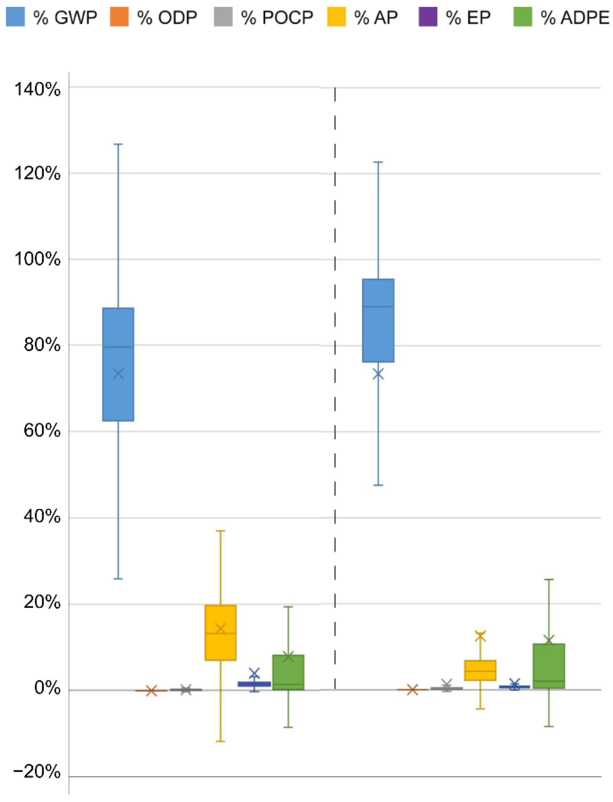
3.1.1. Structure and Finishes (CG 300)

The diagram showing eLCC per fLCC (Figure 4) reveals that the fLCCs are comparatively close to each other for all variations, with the exception of the two solutions with an exterior curtain wall (CW). At the same time, the eLCCs vary greatly, with a small cluster of eLCCs around 50% of fLCCs.
From these results, we selected five variations for representation in timelines, three of which contain a reinforced concrete structure and two of which contain a wood structure (Figure 1, Table A1). Each of these variations yields an extreme in at least one scenario: they result in give the lowest fLCC (RCC 03), highest fLCC (RCC 06), lowest eLCC (RCC 05) and highest eLCC (Wood 05). We added one solution (Wood 04) because experience with standard LCA calculations has shown that a wood structure with a ventilated façade is a recommended solution based on LCA results. Cumulated cost results for all variations can be found in Table A3 in Appendix B.
Figure 5 shows the development of the fLCC and the eLCC throughout the 50-year study period. The fLCC curves of the wood and concrete options converge, mainly due to the frequent exchange of carpet (every 10 years) and EIFS system (after 40 years). The building with a curtain wall displays the highest fLCC, acerbated by replacement of the curtain wall after 30 years.
We see a striking effect of the price increase in EC on the significance of the end-of-life phases of the different buildings. In the standard end-of-life scenario for wood or other renewable materials, emissions from incineration for energy generation are accounted for in phase C3. Phase D in turn shows a credit for energy generation from renewables. This leads to the eLCC of the wood structures exceeding their fLCC if phase D is not accounted for and to their eLCC being higher than the eLCC of the concrete structures, even if phase D is included.

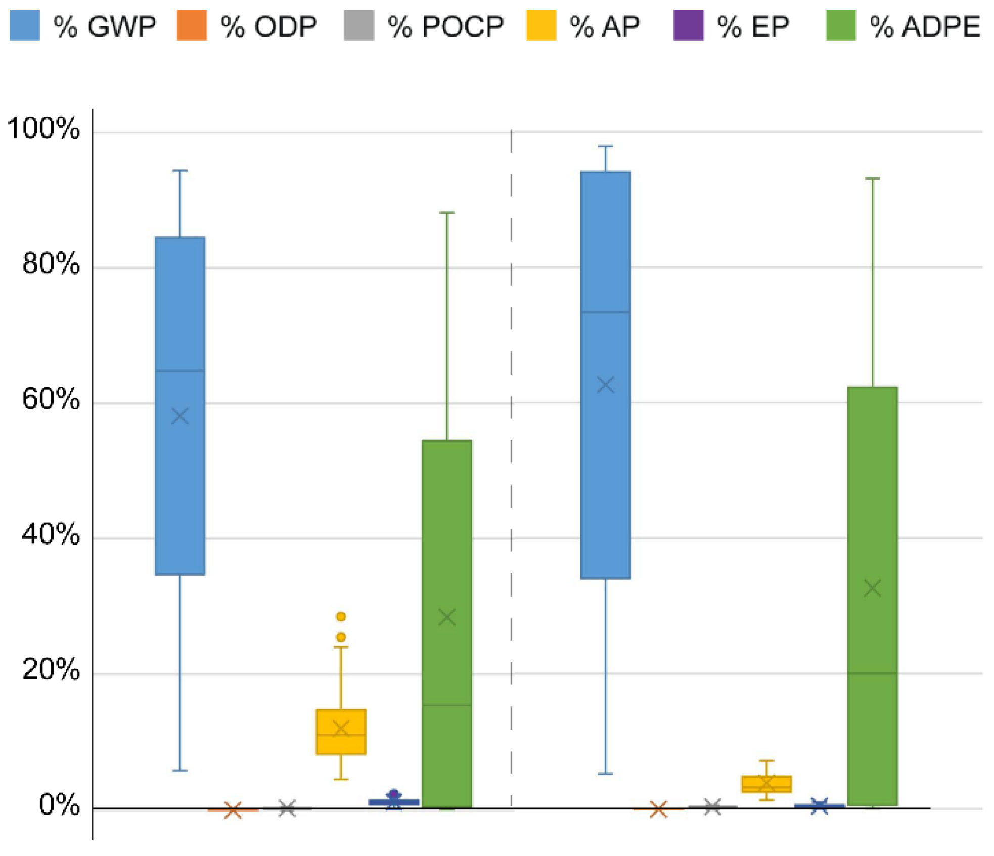
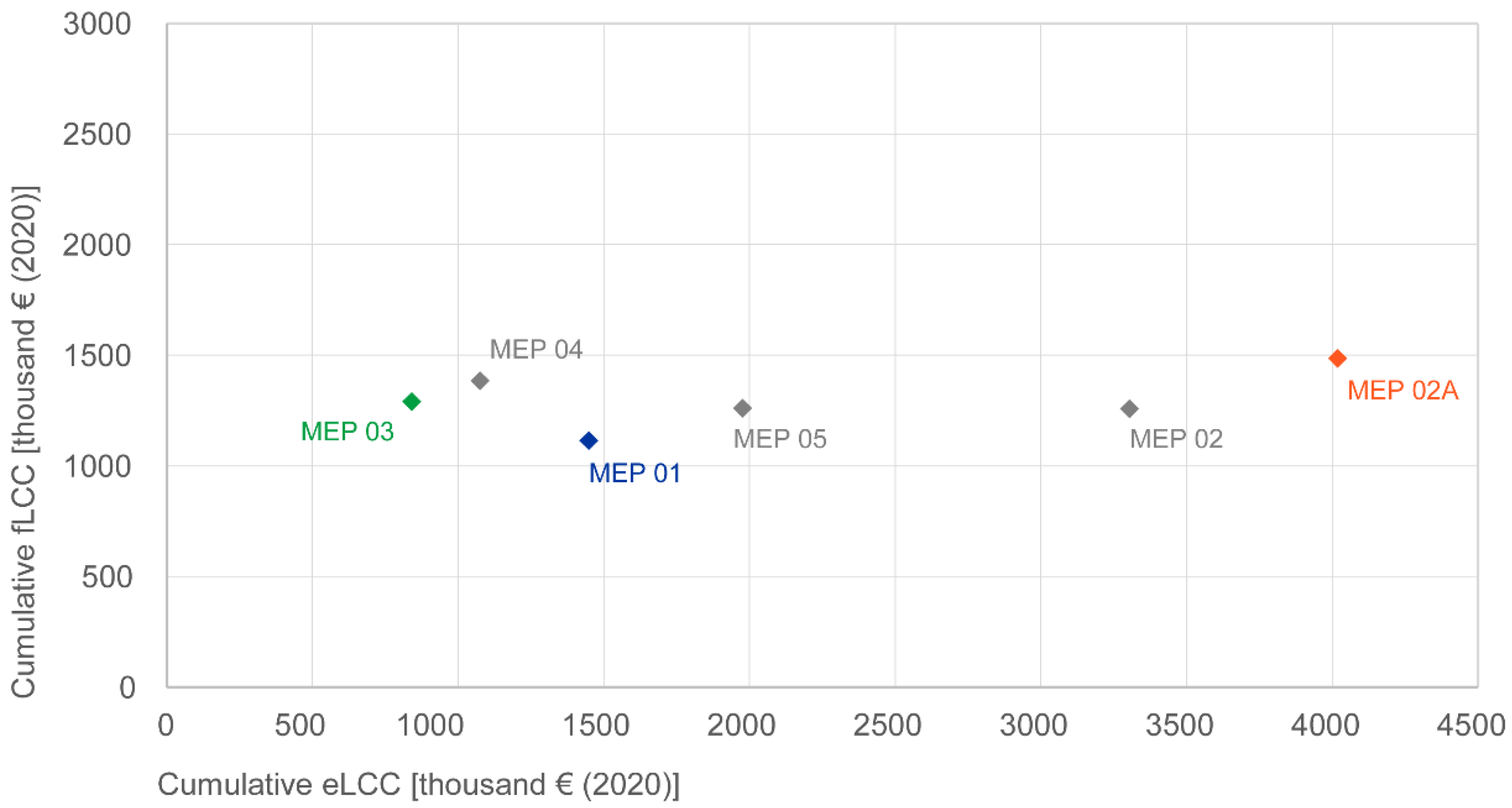
3.1.2. MEP Systems and Operational Phase (CG 400 + B6)

The diagram showing eLCC per fLCC (Figure 6) reveals that for CG 400 + B6, the fLCCs are closer together than the eLCCs for all variations. The difference between eLCCs is greater than for CG 300, and the absolute values exceed the eLCC of CG 300 (Figure 4).
The scenario analysis considers three different energy generation options (Figure 1, Table A2), two renewable energy sources (renewable district heat, MEP 03, and groundwater heat pump, MEP 01) and a non-renewable energy source (gas, MEP 02), the latter with and without PV (MEP 02A). As we recognized that the PV system causes significant amounts of EC in phases A1 to A3 because of its resource depletion potential, we included an option without PV to determine whether emissions savings would offset these costs in the operational phase. These variations yield the extremes: the lowest and highest eLCC and the lowest and highest fLCC. Notably, MEP 02A displays both the highest fLCC and the highest eLCC.
Considering that the same monetary valuation and framework as for the CG 300 investigation applies to CG 400 + B6, the most significant difference between the two building subsystems is the fact that all but one variation display higher eLCCs over their lifetime than fLCCs, even if phase D is included in the calculation (Figure 7). This is due to the high EC caused by the burning of fossil fuels which is visible by the comparatively steep slope of the timelines and is even present in the renewable heat supply solutions due to the electricity mix. Moreover, the ratio of environmental cost of parts of the MEP systems (e.g., PV cells, copper cables) to the financial cost is higher than for building materials (CG 300).
Here, the inclusion or exclusion of phase D also has a significant impact, as the recycling potential of the materials contained in MEP systems (first and foremost metals) is high. As several MEP elements have a relatively short reference service life (RSL) by standard definitions, e.g., PV cellsare replaced every 20 years [53], this also heavily influences phase B4. The timeline representation makes this visible with a steeper or flatter slope at every exchange point of an element, depending on whether phase D is excluded or included. It is also clear that under standard framework conditions, the PV systems’ EC are offset by their emissions savings in relation to the standard electricity mix, despite the gradual improvement in electricity mix and regardless of whether phase D is included or not.

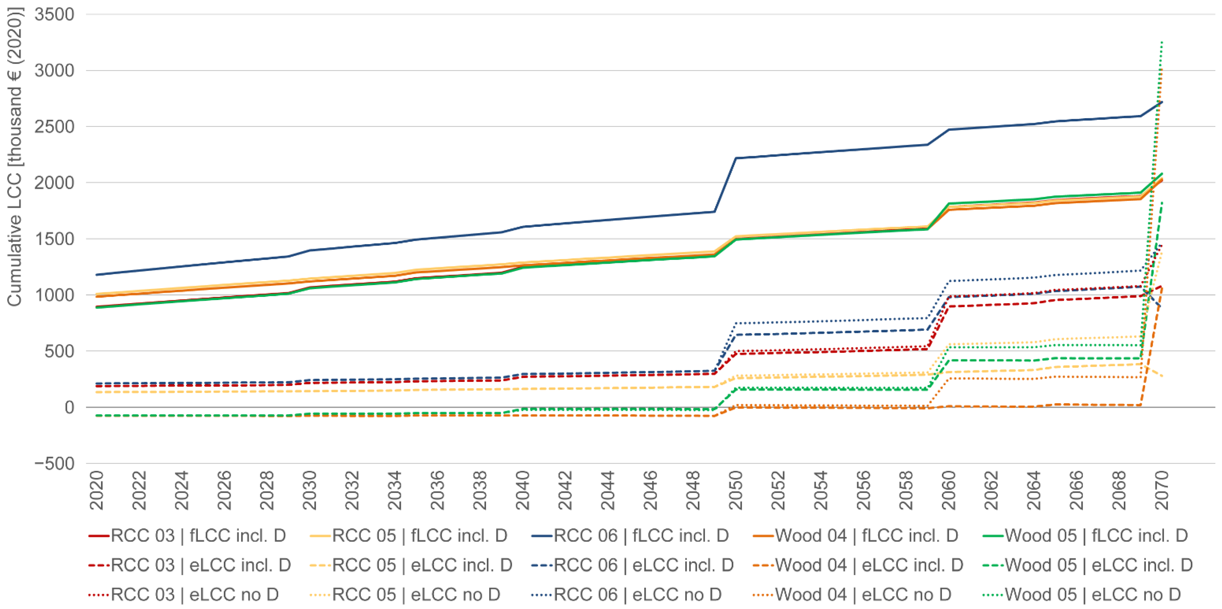
3.2. Temporal Dimension: Scenario Analysis

We varied the temporal dimensions (discount rates and price changes) according to the scenarios in Table 4 to answer the question whether and how introducing the temporal dimension in LCA influences results.

3.2.1. Structure and Finishes (CG 300)

In addition to the expected result that the overall cumulative costs (present value) increase with lower time preference and higher price increase rates (Figure 8), the scenarios change the ranking of the different variations according to their total cost (eLCC + fLCC). We observe that adding eLCC and fLCC provides a better direction towards solutions with lower environmental cost than considering eco-efficiency. Eco-efficiency is seemingly favorable for options with high fLCC, implying that higher financial investment allows for higher emissions. The recommended solution based on fLCC is only identical to the recommended solution based on total cost, if it is identical to the solution with the lowest eLCC (RCC 05 in the low-TP scenario without D). In all other cases, adding eLCC to fLCC changes the recommended solution. However, the scenario choice influences the ranking according to fLCC, as well as according to total cost (with or without D). This implies that a potential recommendation to a client strongly depends on the scenario.
Overall, the choice of time preference scenario has a greater impact on eLCC than on fLCC, as the end-of-life phases play a more significant role in environmental than in economic considerations. Comparing all building variations in all scenarios regarding their total cost (Table A3, Table A4 and Table A5 in Appendix B), variations with a wood structure outperform those with a reinforced concrete structure only for the scenario with high TP if phase D is included. Hybrid variation RCC 05 ranks first in the standard and low-TP scenario if phase D is included; it still ranks high (rank 3 of 13) in the high-TP scenario. If phase D is excluded, the recommendation stays the same for the standard and low-TP scenario but changes for the high-TP scenario.

3.2.2. MEP Systems and Building Operation (CG 400 + B6)

In contrast to the building’s structure and finishes, the choice of temporal parameters changes the eco-efficiency and total cost in absolute terms but does not change the ranking of the different solutions (Figure 9). This is true for all solutions considered, not just the four solutions shown in Figure 9 (Table A6, Table A7 and Table A8 in Appendix B). This observation can be explained by the fact that the operational phase with regularly recurring costs and emissions is the decisive factor for this investigation, unlike the end-of-life phase, which occurs only at one point in the future, when discounting and price increases have their full effect.
As a second notable difference between the two subsystems, CG 300 and CG 400 + B6, we observe that despite the same monetary valuation system, the eLCCs of the MEP systems and phase B6 exceed their fLCCs in all scenarios except for MEP 03 if phase D is included. This occurs quickly (within 9 to 14 years) for MEP 02 and MEP 02A and later in the lifetime of the building (20 years) for MEP 01. In contrast, for the building’s structure and finishes, the eLCCs stay below the fLCCs for most of the building’s lifetime and only exceed fLCC for the low-TP scenario toward the end of the study period. In the standard scenario, this occurs only for the wood buildings if phase D is excluded (Figure 5).

3.3. Implications of Monetary Valuation

3.3.1. Weighting Environmental Impact Indicators

In terms of the relevant indicators and the ratio between life cycle ecological costs and life cycle financial costs, major differences appear between (Table 5):
  • the building’s structural and finish materials (CG 300);
  • MEP systems (HVAC systems, electrical systems and sanitary installations: CG 400); and
  • operational energy use (life cycle phase B6).
For CG 300, global warming potential (GWP) is responsible for the largest share of eLCC, followed by the cost of resource depletion (ADPE). The use case variations show that external costs amount to 14% to 157% of the building’s life cycle cost, depending on the materials used and, on the question, whether life cycle phase D (benefits and loads outside of the system boundary) is included in the calculations.
Abiotic resource depletion of elements (ADPE) is dominant for the eLCC of CG 400, followed by the eLCC of GWP. This is caused by the use of metals, which show values for ADPE higher than those of other materials by a factor of up to 106. It is one of the particularities of ADPE that single materials cause the largest share of environmental costs, disproportionally to their share in the overall building mass. Compared to the fLCC of the building’s MEP systems, eLCC amounts to −11% to 237%, even more strongly depending on the inclusion or exclusion of phase D than for CG 300. Note that the negative values for fLCC reflect a high ADPE credit for recycling metals.
A proportion of 93% to 98% of the eLCC of building operation are caused by GWP if non-renewable or partially non-renewable energy sources are used. In the case of bio-based energy sources, GWP’s share ranges from 51% to 71%, followed by acidification potential (AP) (up to 31%). Overall, environmental costs amount to up to 568% of the life cycle operational costs, strongly depending on the share of non-renewable energy sources used. As many countries are starting to tax CO2 emissions associated with building operation, this is important information for stakeholders. By decarbonizing the energy supply system of the building at a comparatively low cost premium, environmental costs of building operation can be reduced to a minimum, as confirmed by previous studies [54].

3.3.2. Varying Monetary Valuation

We varied monetary valuation values, as shown in Table 2, to investigate how the different values affect the eco-efficiency ratio and whether or not this influences the ranking of options if eLCCs were added to fLCCs. We looked at the ranking of options based on fLCC, eLCC, eco-efficiency and total cost (fLCC + eLCC), each with and without phase D. All results are provided in Supplementary Data S1. Generally, within one time preference scenario, the recommendation based on fLCC stays the same, as monetary valuation does not influence the results.
For CG 300, varying monetary valuation changes recommendations based on fLCC + eLCC only in one case. Minimum valuation and high time preference excluding phase D recommends RCC 03 rather than RCC 05, as the difference in eLCC does not make up for the difference in fLCC. In other words, the monetary valuation model has almost no influence on the ranking of results compared to the considerable influence of time preference scenarios.
For CG 400, recommendations based on fLCC + eLCC remain unchanged between medium and high monetary valuation. At low valuation, recommendations shift towards the solutions with lower fLCC (MEP 01), although MEP 03 remains the solution with the lowest eLCC.
At minimum valuation and low time preference, we observe that the eLCC results in negative values if phase D is included, implying a savings of eLCC because of the high price increase in environmental costs in 50 years.

4. Discussion

4.1. Gaps and Limitations of the Use Case

When applying the framework, several gaps that have not been previously addressed provide opportunities for further research. First, the sensitivity analysis conducted for temporal parameters and monetary values could incorporate further aspects of life cycle uncertainty. Previous studies have addressed single parameters in LCA and/or LCC, such as service lives of elements [55], building lifespan [56,57], material data [58] or design vagueness [20,59]. Experience from these studies can inform a more global sensitivity study on influential parameters. Second, the data gaps identified in [9] also became apparent in this study. The database used in this study, Oekobaudat, provides only limited data on project-specific life cycle phases, such as transport, construction and disassembly (A4, A5, C1 and C2). Data on environmental impacts and cost of MEP systems is sparse and not well-structured; for example, functional units (e.g., kg of ducts) do not lend themselves to early design exploration. Available as-built information about the case study made it possible to consider these data, but further work is required to enable consideration of embedded impacts of MEP systems in a real-life design process. Data gaps in LCC pertain to the end-of-life phases, and cost for disassembly vs. conventional demolition processes is lacking, as well as disposal, reuse, recycling cost or value. For this study, we attached end-of-life costs to building parts and surfaces in order to account for replacement processes. Although we used the same costs for end-of-life processes—at the risk of overestimating these costs, as they are tantamount to an elaborate disassembly process—these costs only play a minor role in the fLCC calculations. However, with increasing cost of landfills and decreasing resource availability, end-of-life costs could contribute significantly to fLCC. In summary, establishing a sound database for both LCA and LCC in parallel would be beneficial for the accuracy and true harmonization of the two methods. This database should close the mentioned data gaps and, ideally, contain information about building parts with different material configurations and building operation. Third, we excluded the mutual influence of MEP systems, energy standard and construction materials to detect differences in the scenario analysis. However, a more extensive variant study could reveal further dependencies and, ideally, win–win situations.
The case study is representative of small office buildings in Germany. The small size and homogenous use profile limited complexity to enable many variations in a manual process. However, the framework can be used on larger-scale buildings and mixed-use developments requiring digital methods to handle the complexity of interdependencies.

4.2. Quasi-Dynamic LCA

The quasi-dynamic approach provides a method to introduce a time horizon into LCA without the necessity of recalculating all underlying data. It reveals a striking influence of the choice of temporal parameters on life cycle results and related recommendations. The low-time-preference scenario implies that future costs and emissions weigh more heavily than present costs and emissions, whereas the high-time-preference scenario focuses on saving costs and emissions now rather than in the future. Both scenarios are worth considering. Given the sense of urgency caused by signs of increasing environmental and social problems resulting from global warming, the high-time-preference scenario can be justified by the argument that if we manage to avoid enough emissions and the resulting serious environmental and economic consequences now, saving emissions in the future could be regarded as less important. Following this logic, deferring emissions should be prioritized, e.g., using wood as a construction material and thereby using buildings as a long-term carbon sink [60]. Under the low-time-preference scenario, the opposite would be the case, resulting in a contradictory recommendation: it is better to cause higher emissions now to save emissions later, while these same (present) emissions might tip the scale towards more serious environmental problems.
In all scenarios, the inclusion or exclusion of end-of-life credits has a significant impact, especially on options with large amounts of wood or metals. This is in line with results from the literature suggesting that wood and steel options are more sensitive towards changes in discount rates due to significant credits in the end-of-life phases [33].
Introducing the time horizon by a quasi-dynamic approach into LCA calculation poses the challenge that emissions evaluation of future processes is based on emissions of current processes. It should be further developed to a truly dynamic method, adding scenarios for future developments in background systems, such as the electricity mix, technological advancements [17] and the time horizon for impacts [15]. In this study, we included a dynamic factor for the electricity mix, as scenarios for the German electricity mix exist. Transferring this scenario to manufacturing processes would require an overall building sector scenario, information about the share of electricity used in manufacturing processes and a dynamic recalculation of environmental data for manufacturing building materials. Such a future scenario might also question the assumption that the same materials and MEP systems, rather than more advanced solutions, replace current technologies at the end of their service life.
Furthermore, the quasi-dynamic approach shows how the length of the study period could be highly significant for decisions made in the design process. The length of the study period represents the potential lifetime of the building, which is subject to a multitude of factors and can therefore vary greatly. The representation of the life cycle in a timeline enables LCA and LCC consultants to discuss the building’s life cycle with regard to a client’s investment horizon, providing insights into credits and liabilities (both in financial and environmental terms) for a future owner and/or user of the building.

4.3. Monetary Weighting

Despite providing valuable insight into the weighting of different environmental indicators and the ratio between life cycle (market) costs and environmental costs, monetizing LCA results bears the danger of underestimating damage to ecosystems and society. Moreover, it runs the risk of suggesting that paying a fee can avoid or mitigate environmental damage. Communication to stakeholders should therefore clearly state that environmental costs are theoretical costs used to summarize the results of ecological calculations, which are likely to be incomplete. For example, building LCA in Germany disregards toxicity because of the lack of agreed-upon and methodologically robust indicators. Additionally, the underlying weighting system and the contribution of single indicators need to be transparent. In this way, monetary valuation identifies the main drivers of EC of buildings, providing guidance towards high emission reduction potentials.
The monetary weighting system used in this study is based on previous work by the authors [13], using the maximum values found in the literature. Including other midpoint impacts beyond GWP in monetary valuation allows for a broader picture than monetizing carbon emissions only. However, it also reveals that GWP largely determines the EC of building materials. Hence, the scenario choices have the largest influence on those building variations with a large share of carbon emissions occurring in the future, i.e., with a large share of renewable materials. How these are evaluated depends, in turn, on both the end-of-life scenarios for these materials and, more importantly, the biogenic carbon accounting method used. As Oekobaudat accounts for biogenic carbon storage in phase A1, for the release of carbon in phase C3 (incineration for energy generation) and for credits due to energy generation in phase D, carbon storage is equivalent to deferring emissions. As Resch et al. [15] point out, a dynamic approach to GWP provides further insight into the effect of delaying emissions. It is the subject of future research to investigate further scenarios with dynamic carbon accounting, as described by Hoxha et al. [61] using the Eco2 framework to couple the scenarios with economic considerations.
The case study combines MEP systems and building operation (phase B6), as these are mutually dependent. The different solutions regarding the energy generation system show that embedded emissions of the MEP systems are dwarfed by the emissions in phase B6 during the 50-year study period. A particularity of MEP systems in comparison to the building’s structure and finishes is the predominance of resource depletion. For the PV system, this leads to the EC of phase A1–A3 exceeding the investment cost of the system. However, emissions-free electricity offsets this EC in comparison to the general electricity mix. Further investigation into the magnitude of the EC of resource depletion is necessary to gain a better understanding of this process.
Lastly, we asked the question of whether adding monetary values for environmental impacts can tip the scale towards lower emission solutions if these prove to have higher life cycle costs than solutions with higher emissions. Overall, we found that changing monetary valuation has a lesser influence on results based on total cost than time preference does. Given the high uncertainty in monetary valuation, this encourages the use of monetary valuation, as in most cases, adding eLCC to fLCC provides leverage towards emission-saving solutions. Additionally, for CG 300 in the high-time-preference scenarios, the solution with the lowest eLCC is also the solution with lowest fLCC, representing a win–win situation. Adding eLCC to fLCC in this case only increases the difference between solutions.
For the building’s MEP systems and operational energy use, the preferred solution is the one with the lowest eLCC if medium or high monetary valuation is used. For low valuation, this solution is only preferred at high TP. We conclude that medium or high valuation of environmental impacts gives enough weight to emissions to provide leverage towards lower emissions. Moreover, adding eLCC to fLCC appears to be a valuable strategy for identifying solutions that minimize both fLCC and eLCC.

5. Conclusions

Calculating LCA and LCC in parallel requires extensive background data, as well as expertise and time, which is often a sparse resource in regular design processes. Therefore, we developed an Eco2 framework in a previous study to structure the integrated process. This second part of the study tests the Eco2 framework in a fictitious building design process based on a real-life case study of a small-scale office building.
Collecting the background data for the case study closes some typical LCA and LCC data gaps and lays the groundwork for a common environmental–economic database. It also reveals that different types of data need to be associated with various aggregation levels of building materials, building parts or the whole building. Extending this project-specific data collection to a more widely usable database enables a design supported by Eco2.
Considering discounting and price changes in LCA and thus adding a temporal dimension is not a standard procedure in current LCA calculations, which use a static approach and show total emissions, at best, by life cycle phase and at worst as a total sum. Varying the temporal parameters assists practitioners in discussing time preference not only in economic but also environmental terms. The case study shows that the choice of time preference scenario decisively influences potential recommendations regarding the building’s structure and finishes but leaves recommendations regarding the MEP systems largely unchanged. This implies that time preference is less important for MEP systems than for building materials, as the choice of MEP systems, in effect, determines emissions in the operational phase, which recur regularly. For building materials with high emission values and credits in the end-of-life phases (e.g., wood and metals), varying the temporal parameters and including or excluding credits (phase D) has a great influence on environmental life cycle costs because these are incurred at one point in the distant future, when the exponential effect of temporal parameters is largest.
Applying different monetary values for emissions as a form of weighting of the environmental indicators and as a “counterweight” to economic results affects the total cost (environmental and financial life cycle cost, eLCC+fLCC). In the case study, adding eLCC to fLCC shifts recommendations from the solutions with the lowest fLCC to solutions with the lowest eLCC unless a very low valuation of emissions is used. It also reveals win–win solutions with both low fLCC and low eLCC.
The eLCC of MEP systems and energy use in operation tend to exceed the fLCC of MEP systems and energy use. This leads to the conclusion that this factor remains extremely influential for the overall life cycle performance of a building, even with an ambitious energy standard. It implies that the choice of MEP system is the decision with the most leverage in environmental terms without being economically disadvantageous. As GWP dominates the EC of building operation, this is in line with previous studies and policy recommendations identifying renewable energy systems as the most economically efficient emissions-saving strategy.

Supplementary Materials

The following supporting information can be downloaded at: https://www.mdpi.com/article/10.3390/su14106025/s1.

Author Contributions

Conceptualization, methodology, formal analysis, investigation and data curation: P.S.-M.; writing—original draft preparation: P.S.-M.; writing—review and editing: W.L.; visualization: P.S.-M.; supervision: W.L.; funding acquisition: W.L. and P.S.-M. All authors have read and agreed to the published version of the manuscript.

Funding

This research was funded by the Deutsche Forschungsgemeinschaft (German Research Foundation, DFG) under grant FOR2363 (project number 271444440).

Acknowledgments

We thank Ferdinand Tausendpfund GmbH for allowing us to use their office building as a case study, in particular for the valuable and detailed information about the building’s MEP systems. Thank you to Anne Winkelkotte for her Master thesis work, which inspired part of this research, and to Tanja Stocker for her assistance in grouping Oekobaudat data. For their scientific input and valuable feedback, we sincerely thank Leander Schneider and Inger Andresen. Last but not least, we thank four anonymous reviewers for their valuable feedback.

Conflicts of Interest

The authors declare no conflict of interest.

Abbreviations

APacidification potential
ADPEabiotic depletion potential of elements
BIMbuilding information modelling
BNBBewertungssystem nachhaltiges Bauen (building sustainability evaluation system)
DGNBDeutsche Gesellschaft für nachhaltiges Bauen (German sustainable building council)
ECenvironmental cost
eLCCenvironmental life cycle cost
EPeutrophication potential
fLCCfinancial life cycle cost
GHGgreenhouse gas
GWPglobal warming potential
HVACheating, ventilation, air conditioning
LCAlife cycle assessment
LCClife cycle costing
MEPmechanical, electrical, plumbing
NPCnet present cost
ODPozone depletion potential
POCPphotochemical ozone creation potential
PVphotovoltaic
RSLreference service life
TPtime preference

Appendix A. Case Study Specifications

Table A1. Characteristics of the variations in the building’s structure and finishes shown in the timelines. RCC: reinforced concrete; SL brick: sand–lime brick; EIFS: exterior insulation and finish system; EPS: expanded polystyrene; PVC polyvinyl chloride.
Variation NameStructureExt. Wall CoreExt. Wall
Finish
Window FramesInsulation Material
Int. Floors
Floor
Finish
Interior Load-Bearing WallsInterior Non-Load-Bearing Walls
RCC 03RCCSL brickEIFS (EPS)PVCEPScarpetmasonrymetal stud drywall
RCC 05RCCWood frameVentilated (alum. siding)woodwood fiberwood parquetmasonrywood stud drywall
RCC 06RCCCurtain wall (alu.)Aluminum siding(alum.)EPScarpetmasonrymetal stud drywall
Wood 04Solid woodWood frameVentilated (alum. siding)woodwood fiberwood parquetsolid woodwood stud drywall
Wood 05Solid woodWood frameEIFS (wood fiber)PVCEPScarpetsolid woodmetal stud drywall
Table A2. Characteristics of the variations in the building’s energy supply system shown in the timelines.
Variation NameHeating SupplyCooling SupplyPV
MEP 01Groundwater heat pumpCompression (electricity)yes
MEP 02Gas condensing boilerCompression (electricity)yes
MEP 02AGas condensing boilerCompression (electricity)no
MEP 03Renewable district heatCompression (electricity)yes

Appendix B. Case Study Results: Medium Monetary Valuation

Table A3. Comparison of all variations in CG 300 (standard scenario) (1). The colors indicate the lowest (green) and highest values (red), gradation for the ranking in-between.
VariationeLCC (No D)eLCC (Incl. D)fLCCeLCC No D/fLCCeLCC Incl. D/LCC
RCC 011,454,277€1,067,346€2,098,014€69.3%50.9%
RCC 01A1,351,859€1,026,404€2,110,477€64.1%48.6%
RCC 021,328,615€990,597€2,044,960€65.0%48.4%
RCC 02A1,283,670€967,248€2,049,106€62.6%47.2%
RCC 02B1,398,825€932,434€2,068,703€67.6%45.1%
RCC 031,448,969€1,080,746€2,020,972€71.7%53.5%
RCC 041,450,918€744,124€2,059,883€70.4%36.1%
RCC 051,386,873€279,927€2,038,062€68.0%13.7%
RCC 061,465,022€880,698€2,717,295€53.9%32.4%
Wood 043,043,717€1,058,493€2,027,408€150.1%52.2%
Wood 04A3,170,602€1,408,453€2,048,539€154.8%68.8%
Wood 053,266,101€1,819,585€2,079,617€157.1%87.5%
Wood 063,159,066€1,283,054€2,651,549€119.1%48.4%
VariationfLCC + eLCC
(No D)
fLCC + eLCC
(Incl. D)
Ranking Based on fLCCRanking Based on fLCC + eLCC No DRanking Based on fLCC + eLCC Incl. D
RCC 013,552,291€3,165,360€1089
RCC 01A3,462,336€3,136,881€1148
RCC 023,373,575€3,035,557€425
RCC 02A3,332,777€3,016,355€614
RCC 02B3,467,528€3,001,137€853
RCC 033,469,941€3,101,718€167
RCC 043,510,800€2,804,007€772
RCC 053,424,935€2,317,989€331
RCC 064,182,317€3,597,993€13911
Wood 045,071,124€3,085,900€2106
Wood 04A5,219,141€3,456,992€51110
Wood 055,345,719€3,899,203€91212
Wood 065,810,615€3,934,603€121313
Table A4. Comparison of all variations in CG 300 (high-time-preference scenario) (2). The colors indicate the lowest (green) and highest values (red), gradation for the ranking in-between.
VariationeLCC (No D)eLCC (Incl. D)fLCCeLCC No D/fLCCeLCC Incl. D/LCC
RCC 01542,878€463,417€1,543,833€35.2%30.0%
RCC 01A522,332€455,761€1,552,990€33.6%29.3%
RCC 02510,346€440,888€1,505,893€33.9%29.3%
RCC 02A498,599€433,668€1,508,939€33.0%28.7%
RCC 02B516,114€419,739€1,523,337€33.9%27.6%
RCC 03537,319€461,208€1,479,057€36.3%31.2%
RCC 04525,496€387,226€1,523,891€34.5%25.4%
RCC 05422,631€201,149€1,528,473€27.7%13.2%
RCC 06591,671€464,252€1,992,432€29.7%23.3%
Wood 04526,262€145,253€1,507,964€34.9%9.6%
Wood 04A513,725€176,521€1,498,082€34.3%11.8%
Wood 05615,922€344,207€1,494,950€41.2%23.0%
Wood 06631,454€258,236€1,950,873€32.4%13.2%
VariationfLCC + eLCC
(No D)
fLCC + eLCC
(Incl. D)
Ranking Based on fLCCRanking Based on fLCC + eLCC No DRanking Based on fLCC + eLCC Incl. D
RCC 012,086,711€2,007,250€101010
RCC 01A2,075,321€2,008,750€11911
RCC 022,016,239€1,946,781€449
RCC 02A2,007,538€1,942,607€627
RCC 02B2,039,451€1,943,076€778
RCC 032,016,376€1,940,265€156
RCC 042,049,387€1,911,117€885
RCC 051,951,104€1,729,622€913
RCC 062,584,102€2,456,684€131313
Wood 042,034,226€1,653,217€561
Wood 04A2,011,808€1,674,603€332
Wood 052,110,872€1,839,157€2114
Wood 062,582,327€2,209,109€121212
Table A5. Comparison of all variations in CG 300 (low-time-preference scenario) (3). The colors indicate the lowest (green) and highest values (red), gradation for the ranking in-between.
VariationeLCC (No D)eLCC (Incl. D)fLCCeLCC No D/fLCCeLCC Incl. D/LCC
RCC 015,273,049€3,325,161€3,473,354€152%96%
RCC 01A4,765,285€3,116,764€3,494,411€136%89%
RCC 024,693,824€2,989,530€3,376,265€139%89%
RCC 02A4,497,741€2,898,623€3,383,270€133%86%
RCC 02B5,122,728€2,793,300€3,416,381€150%82%
RCC 035,270,709€3,426,129€3,359,262€157%102%
RCC 045,466,532€1,784,772€3,381,828€162%53%
RCC 056,030,094€389,459€3,331,686€181%12%
RCC 064,820,728€1,966,446€4,408,017€109%45%
Wood 0416,343,445€5,900,299€3,354,515€487%176%
Wood 04A17,225,915€7,963,048€3,462,528€497%230%
Wood 0516,886,119€9,170,541€3,546,134€476%259%
Wood 0616,030,523€6,352,276€4,331,642€370%147%
VariationfLCC + eLCC
(No D)
fLCC + eLCC
(Incl. D)
Ranking Based on fLCCRanking Based on fLCC + eLCC No DRanking Based on fLCC + eLCC Incl. D
RCC 018,746,403€6,798,514€969
RCC 01A8,259,697€6,611,175€1037
RCC 028,070,089€6,365,795€425
RCC 02A7,881,011€6,281,893€614
RCC 02B8,539,110€6,209,681€743
RCC 038,629,972€6,785,391€358
RCC 048,848,360€5,166,600€572
RCC 059,361,780€3,721,145€191
RCC 069,228,746€6,374,463€1386
Wood 0419,697,961€9,254,814€21010
Wood 04A20,688,443€11,425,575€81312
Wood 0520,432,253€12,716,675€111213
Wood 0620,362,165€10,683,919€121111
Table A6. Comparison of all variations in CG 400 + B6 (standard scenario) (1). The colors indicate the lowest (green) and highest values (red), gradation for the ranking in-between.
VariationeLCC (No D)eLCC (Incl. D)fLCCeLCC No D/fLCCeLCC Incl. D/LCC
MEP 012,981,472€1,448,856€1,115,159€267%130%
MEP 024,766,964€3,303,755€1,259,252€379%262%
MEP 02A5,026,850€4,018,056€1,486,969€338%270%
MEP 032,288,667€839,932€1,291,476€177%65%
MEP 042,540,220€1,074,498€1,384,925€183%78%
MEP 053,441,577€1,975,856€1,259,789€273%157%
VariationfLCC + eLCC
(No D)
fLCC + eLCC
(Incl. D)
Ranking Based on fLCCRanking Based on fLCC + eLCC No DRanking Based on fLCC + eLCC Incl D
MEP 014,096,632€2,564,015€133
MEP 026,026,216€4,563,007€255
MEP 02A6,513,819€5,505,026€666
MEP 033,580,143€2,131,408€411
MEP 043,925,144€2,459,423€522
MEP 054,701,366€3,235,645€344
Table A7. Comparison of all variations in CG 400+B6 (high-time-preference scenario) (2). The colors indicate the lowest (green) and highest values (red), gradation for the ranking in-between.
VariationeLCC (No D)eLCC (Incl. D)fLCCeLCC No D/fLCCeLCC Incl. D/LCC
MEP 011,088,355€710,178€694,507€157%102%
MEP 021,682,423€1,321,373€735,427€229%180%
MEP 02A1,774,694€1,525,775€798,743€222%191%
MEP 03842,553€485,090€744,455€113%65%
MEP 04929,199€567,529€796,000€117%71%
MEP 051,259,322€897,652€748,330€168%120%
VariationfLCC + eLCC
(No D)
fLCC + eLCC
(Incl. D)
Ranking Based on fLCCRanking Based on fLCC + eLCC No DRanking Based on fLCC + eLCC Incl D
MEP 011,782,862€1,404,685€133
MEP 022,417,850€2,056,800€255
MEP 02A2,573,437€2,324,518€666
MEP 031,587,008€1,229,545€311
MEP 041,725,199€1,363,529€522
MEP 052,007,652€1,645,982€444
Table A8. Comparison of all variations in CG 400+B6 (low-time-preference scenario) (2). The colors indicate the lowest (green) and highest values (red), gradation for the ranking in-between.
VariationeLCC (No D)eLCC (Incl. D)fLCCeLCC No D/fLCCeLCC Incl. D/LCC
MEP 0110,031,652€3,109,839€2,275,466€441%137%
MEP 0216,407,963€9,798,936€2,795,097€587%351%
MEP 02A17,328,600€12,767,399€3,623,491€478%352%
MEP 037,662,784€1,118,765€2,912,465€263%38%
MEP 048,539,929€1,919,577€3,130,728€273%61%
MEP 0511,558,841€4,938,490€2,741,389€422%180%
VariationfLCC + eLCC
(No D)
fLCC + eLCC
(Incl. D)
Ranking Based on fLCCRanking Based on fLCC + eLCC No DRanking Based on fLCC + eLCC Incl D
MEP 0112,307,118€5,385,305€133
MEP 0219,203,060€12,594,033€255
MEP 02A20,952,091€16,390,891€666
MEP 0310,575,249€4,031,229€311
MEP 0411,670,656€5,050,305€522
MEP 0514,300,230€7,679,879€444

Appendix C. Weighting of Oekobaudat 2020-II Data by Monetary Valuation

Figure A1. Weighting of ecological indicators resulting from minimum (left) and maximum (right) monetary valuation for CG 300 and life cycle phases A1–A3, based on Oekobaudat 2020-II [26].
Sustainability 14 06025 g0a1
Figure A2. Weighting of ecological indicators resulting from minimum (left) and maximum (right) monetary valuation for CG 400 and life cycle phases A1–A3, based on Oekobaudat 2020-II [26].
Sustainability 14 06025 g0a2
Figure A3. Weighting of ecological indicators resulting from minimum (left) and maximum (right) monetary valuation for life cycle phase B6 (non-renewable sources), based on Oekobaudat 2020-II [26].
Sustainability 14 06025 g0a3
Figure A4. Weighting of ecological indicators resulting from minimum (left) and maximum (right) monetary valuation for life cycle phase B6 (renewable sources), based on Oekobaudat 2020-II [26].
Sustainability 14 06025 g0a4

References

  1. Global Alliance for Buildings and Construction, International Energy Agency (IEA) and the United Nations Environment Programme. 2021 Global Status Report for Buildings and Construction; IEA: Paris, France, 2021. [Google Scholar]
  2. Eurostat. Material Flow Accounts Statistics—Material Footprints. Available online: https://ec.europa.eu/eurostat/statistics-explained/SEPDF/cache/36609.pdf (accessed on 30 March 2022).
  3. IEA, International Energy Agency. World Energy Outlook. 2021. Available online: https://iea.blob.core.windows.net/assets/4ed140c1-c3f3-4fd9-acae-789a4e14a23c/WorldEnergyOutlook2021.pdf (accessed on 16 February 2022).
  4. Ghisellini, P.; Ripa, M.; Ulgiati, S. Exploring environmental and economic costs and benefits of a circular economy approach to the construction and demolition sector. A literature review. J. Clean. Prod. 2018, 178, 618–643. [Google Scholar] [CrossRef]
  5. Publications Office. Directive (EU) 2018/ of The European Parliament and of the Council of 30 May 2018 Amending Directive 2010/31/EU on The Energy Performance of Buildings and Directive 2012/27/EU on Energy Efficiency; Official Journal of the European Union L 156/91; European Union: Maastricht, The Netherlands, 2018. [Google Scholar]
  6. Bahramian, M.; Yetilmezsoy, K. Life cycle assessment of the building industry: An overview of two decades of research (1995–2018). Energy Build. 2020, 219, 109917. [Google Scholar] [CrossRef]
  7. Goh, B.H.; Sun, Y. The development of life-cycle costing for buildings. Build. Res. Inf. 2015, 44, 319–333. [Google Scholar] [CrossRef]
  8. França, W.T.; Barros, M.V.; Salvador, R.; de Francisco, A.C.; Moreira, M.T.; Piekarski, C.M. Integrating life cycle assessment and life cycle cost: A review of environmental-economic studies. Int. J. Life Cycle Assess. 2021, 26, 244–274. [Google Scholar] [CrossRef]
  9. Schneider-Marin, P.; Winkelkotte, A.; Lang, W. Integrating Environmental and Economic Perspectives in Building Design. Sustainability 2022, 14, 4637. [Google Scholar] [CrossRef]
  10. Islam, H.; Jollands, M.; Setunge, S. Life cycle assessment and life cycle cost implication of residential buildings—A review. Renew. Sustain. Energy Rev. 2015, 42, 129–140. [Google Scholar] [CrossRef]
  11. Hester, J.; Gregory, J.; Ulm, F.-J.; Kirchain, R. Building design-space exploration through quasi-optimization of life cycle impacts and costs. Build. Environ. 2018, 144, 34–44. [Google Scholar] [CrossRef]
  12. European Commission. Ecodesign and Energy Labelling. Available online: https://ec.europa.eu/growth/single-market/european-standards/harmonised-standards/ecodesign_en (accessed on 30 March 2022).
  13. Schneider-Marin, P.; Lang, W. Environmental costs of buildings: Monetary valuation of ecological indicators for the building industry. Int. J. Life Cycle Assess. 2020, 25, 1637–1659. [Google Scholar] [CrossRef]
  14. Stevanovic, M.; Allacker, K.; Vermeulen, S. Development of an Approach to Assess the Life Cycle Environmental Impacts and Costs of General Hospitals through the Analysis of a Belgian Case. Sustainability 2019, 11, 856. [Google Scholar] [CrossRef] [Green Version]
  15. Resch, E.; Andresen, I.; Cherubini, F.; Brattebø, H. Estimating dynamic climate change effects of material use in buildings—Timing, uncertainty, and emission sources. Build. Environ. 2020, 187, 107399. [Google Scholar] [CrossRef]
  16. Asdrubali, F.; Baggio, P.; Prada, A.; Grazieschi, G.; Guattari, C. Dynamic life cycle assessment modelling of a NZEB building. Energy 2020, 191, 116489. [Google Scholar] [CrossRef]
  17. Obrecht, T.P.; Jordan, S.; Legat, A.; Passer, A. The role of electricity mix and production efficiency improvements on greenhouse gas (GHG) emissions of building components and future refurbishment measures. Int. J. Life Cycle Assess. 2021, 26, 839–851. [Google Scholar] [CrossRef]
  18. Klauß, S.; Maas, A. Entwicklung einer Datenbank mit Modellgebäuden für Energiebezogene Untersuchungen, Insbesondere der Wirtschaftlichkeit. Forschungsinitiative Zukunft Bau. 2010. Available online: https://www.irbnet.de/daten/baufo/20118035234/Endbericht.pdf (accessed on 14 May 2022).
  19. Abualdenien, J.; Schneider-Marin, P.; Zahedi, A.; Harter, H.; Exner, H.; Steiner, D.; Singh, M.M.; Borrmann, A.; Lang, W.; Petzold, F.; et al. Consistent management and evaluation of building models in the early design stages. J. Inf. Technol. Constr. 2020, 25, 212–232. [Google Scholar] [CrossRef]
  20. Schneider-Marin, P.; Harter, H.; Tkachuk, K.; Lang, W. Uncertainty Analysis of Embedded Energy and Greenhouse Gas Emissions Using BIM in Early Design Stages. Sustainability 2020, 12, 2633. [Google Scholar] [CrossRef] [Green Version]
  21. Vollmer, M.; Harter, H.; Schneider-Marin, P.; Lang, W.; Pfoh, S. Ferdinand Tausendpfund –Lebenszyklusanalyse und Gebäudemonitoring: Innovation; Fakultät für Architektur, Technische Universität München: Munich, Germany, 2019. [Google Scholar]
  22. Abualdenien, J.; Borrmann, A. A meta-model approach for formal specification and consistent management of multi-LOD building models. Adv. Eng. Inform. 2019, 40, 135–153. [Google Scholar] [CrossRef] [Green Version]
  23. Singh, M.M.; Geyer, P. Information requirements for multi-level-of-development BIM using sensitivity analysis for energy performance. Adv. Eng. Inform. 2019, 43, 101026. [Google Scholar] [CrossRef]
  24. Singh, M.M.; Singaravel, S.; Klein, R.; Geyer, P. Quick energy prediction and comparison of options at the early design stage. Adv. Eng. Inform. 2020, 46, 101185. [Google Scholar] [CrossRef]
  25. Harter, H.; Singh, M.M.; Schneider-Marin, P.; Lang, W.; Geyer, P. Uncertainty Analysis of Life Cycle Energy Assessment in Early Stages of Design. Energy Build. 2019, 208, 109635. [Google Scholar] [CrossRef]
  26. BMI. Ökobaudat. Available online: https://www.oekobaudat.de/datenbank/archiv/oekobaudat-2020-ii.html. (accessed on 14 January 2022).
  27. f:data GmbH. Baupreislexikon. Available online: www.baupreislexikon.de (accessed on 11 December 2020).
  28. BKI. BKI Baukosten Positionen Neubau 2020: Statistische Kostenkennwerte für Positionen; BKI: Stuttgart, Germany, 2020; ISBN 978-3-481-04060-4. [Google Scholar]
  29. Weka Media. SIRADOS Baupreishandbuch 2020 Gebäudetechnik; WEKA MEDIA GmbH & Co. KG: Kissing, Germany, 2020; ISBN 978-3-8111-0267-5. [Google Scholar]
  30. Deutsches Institut für Normung e.V. DIN V 18599 Energetische Bewertung von Gebäuden–Berechnung des Nutz-, End- und Primärenergiebedarfs für Heizung, Kühlung, Lüftung, Trinkwarmwasser und Beleuchtung. Beuth Verlag: Berlin, Germany, 2016; (DIN V 18599). [Google Scholar]
  31. Mirzaie, S.; Thuring, M.; Allacker, K. End-of-life modelling of buildings to support more informed decisions towards achieving circular economy targets. Int. J. Life Cycle Assess. 2020, 25, 2122–2139. [Google Scholar] [CrossRef]
  32. Wastiels, L.; van Dessel, J.; Delem, L. Relevance of the recycling potential (module D) in building LCA: A case study on the retrofitting of a house in Seraing. In Proceedings of the WSB14 World Sustainable Building Conference, Barcelona, Spain, 28–30 October 2014. [Google Scholar]
  33. Lu, H.R.; El Hanandeh, A.; Gilbert, B. A comparative life cycle study of alternative materials for Australian multi-storey apartment building frame constructions: Environmental and economic perspective. J. Clean. Prod. 2017, 166, 458–473. [Google Scholar] [CrossRef]
  34. DGNB GmbH. ENV1.1 Oekobilanz des Gebaeudes. DGNB System—Kriterienkatalog Gebäude Neubau; DGNB GmbH: Stuttgart, Germany, 2018. [Google Scholar]
  35. BMVBS. Bewertungssystem Nachhaltiges Bauen (BNB) Bilanzierungsregeln für die Erstellung von Ökobilanzen: Neubau Büro- und Verwaltungsgebäude. 2015. Available online: https://www.bnb-nachhaltigesbauen.de/fileadmin/steckbriefe/verwaltungsgebaeude/neubau/v_2015/LCA-Bilanzierungsregeln_BNB_BN_2015.pdf (accessed on 15 February 2021).
  36. DGNB GmbH. DGNB Kriterium- ECO1.1 Gebaeudebezogene-Kosten-im-Lebenszyklus; DGNB GmbH: Stuttgart, Germany, 2018. [Google Scholar]
  37. BMVBS. Bewertungssystem Nachhaltiges Bauen (BNB) Lebenszykluskosten: 2.1.1 Gebäudebezogene Kosten im Lebenszyklus. 2015. Available online: https://www.bnb-nachhaltigesbauen.de/fileadmin/steckbriefe/verwaltungsgebaeude/neubau/v_2015/BNB_BN2015_211.pdf (accessed on 29 November 2020).
  38. DIN Deutsches Institut für Normung e.V. DIN 276 Kosten im Bauwesen; Building Costs; Beuth Verlag: Berlin, Germany, 2018. [Google Scholar]
  39. GAEB. Standardleistungsbuch Bau. Available online: https://www.gaeb.de/en/products/stlb-bau/ (accessed on 6 June 2021).
  40. Soust-Verdaguer, B.; Martínez, A.G.; Llatas, C.; de Cózar, J.G.; Allacker, K.; Trigaux, D.; Alsema, E.; Berg, B.; Dowdell, D.; Debacker, W.; et al. Implications of using systematic decomposition structures to organize building LCA information: A comparative analysis of national standards and guidelines- IEA EBC ANNEX 72. IOP Conf. Ser. Earth Environ. Sci. 2020, 588, 022008. [Google Scholar] [CrossRef]
  41. Schneider-Marin, P.; Dotzler, C.; Röger, C.; Lang, W.; Glöggler, J.; Meier, K.; Runkel, S. Design2Eco|Schlussbericht: Lebenszyklusbetrachtung im Planungsprozess von Büro- und Verwaltungsgebäuden—Entscheidungsgrundlagen und Optimierungsmöglichkeiten für frühe Planungsphasen; Fraunhofer IRB Verlag: Stuttgart, Germany, 2019. [Google Scholar]
  42. Hollberg, A.; Kiss, B.; Röck, M.; Soust-Verdaguer, B.; Wiberg, A.H.; Lasvaux, S.; Galimshina, A.; Habert, G. Review of visualising LCA results in the design process of buildings. Build. Environ. 2020, 190, 107530. [Google Scholar] [CrossRef]
  43. Hellweg, S.; Hofstetter, T.; Hungerbuhler, K. Discounting and the environment should current impacts be weighted differently than impacts harming future generations? Int. J. Life Cycle Assess. 2003, 8, 8–18. [Google Scholar] [CrossRef]
  44. Hoel, M.; Sterner, T. Discounting and relative prices. Clim. Chang. 2007, 84, 265–280. [Google Scholar] [CrossRef]
  45. Azar, C.; Sterner, T. Discounting and distributional considerations in the context of global warming. Ecol. Econ. 1996, 19, 169–184. [Google Scholar] [CrossRef]
  46. Bünger, B.; Matthey, A. Methodenkonvention 3.0 zur Ermittlung von Umweltkosten: Methodische Grundlagen; Umweltbundesamt: Dessau-Roßlau, Germany, 2018. [Google Scholar]
  47. Matthey, A.; Bünger, B. Methodenkonvention 3.0 zur Ermittlung von Umweltkosten: Kostensätze. Stand 02/2019; Umweltbundesamt: Dessau-Roßlau, Germany, 2019. [Google Scholar]
  48. Weidema, B.P. Using the budget constraint to monetarise impact assessment results. Ecol. Econ. 2009, 68, 1591–1598. [Google Scholar] [CrossRef]
  49. Vogtländer, J. Ecocosts 2017_V1-6 Midpoint Tables. Available online: http://www.ecocostsvalue.com/EVR/model/theory/subject/5-data.html (accessed on 19 November 2019).
  50. Ahlroth, S.; Finnveden, G. Ecovalue08–A new valuation set for environmental systems analysis tools. J. Clean. Prod. 2011, 19, 1994–2003. [Google Scholar] [CrossRef]
  51. Steen, B.; Palander, S. EPS-2015d-Including-Climate-Impacts-from-Secondary-Particles. Available online: https://www.lifecyclecenter.se/publications/eps-2015d1-excluding-climate-impacts-from-secondary-particles/ (accessed on 4 January 2020).
  52. ISO 15686-5; Buildings and Constructed Assets—Service Life Planning; Part 5: Life-Cycle-Costing. International Organization for Standardization: Geneva, Switzerland, 2017.
  53. BBSR. Nutzungsdauern von Bauteilen für Lebenszyklusanalysen nach Bewertungssystem Nachhaltiges Bauen (BNB). 2017. Available online: https://www.nachhaltigesbauen.de/austausch/nutzungsdauern-von-bauteilen/ (accessed on 7 March 2020).
  54. Conci, M.; Konstantinou, T.; Dobbelsteen, A.V.D.; Schneider, J. Trade-off between the economic and environmental impact of different decarbonisation strategies for residential buildings. Build. Environ. 2019, 155, 137–144. [Google Scholar] [CrossRef]
  55. Goulouti, K.; Padey, P.; Galimshina, A.; Habert, G.; Lasvaux, S. Uncertainty of building elements’ service lives in building LCA & LCC: What matters? Build. Environ. 2020, 183, 106904. [Google Scholar] [CrossRef]
  56. Marsh, R. Building lifespan: Effect on the environmental impact of building components in a Danish perspective. Arch. Eng. Des. Manag. 2016, 13, 80–100. [Google Scholar] [CrossRef]
  57. Rauf, A.; Crawford, R.H. Building service life and its effect on the life cycle embodied energy of buildings. Energy 2015, 79, 140–148. [Google Scholar] [CrossRef]
  58. Häfliger, I.-F.; John, V.; Passer, A.; Lasvaux, S.; Hoxha, E.; Saade, M.R.M.; Habert, G. Buildings environmental impacts’ sensitivity related to LCA modelling choices of construction materials. J. Clean. Prod. 2017, 156, 805–816. [Google Scholar] [CrossRef] [Green Version]
  59. Harter, H.; Schneider-Marin, P.; Lang, W. The Energy Grey Zone–Uncertainty in Embedded Energy and Greenhouse Gas Emissions Assessment of Buildings in Early Design Phases. In Proceedings of the Sixth International Symposium on Life-Cycle Civil Engineering (IALCCE 2018), Gent, Belgium, 28–31 October 2018. [Google Scholar]
  60. Churkina, G.; Organschi, A.; Reyer, C.P.O.; Ruff, A.; Vinke, K.; Liu, Z.; Reck, B.K.; Graedel, T.E.; Schellnhuber, H.J. Buildings as a global carbon sink. Nat. Sustain. 2020, 3, 269–276. [Google Scholar] [CrossRef]
  61. Hoxha, E.; Passer, A.; Saade, M.R.M.; Trigaux, D.; Shuttleworth, A.; Pittau, F.; Allacker, K.; Habert, G. Biogenic carbon in buildings: A critical overview of LCA methods. Build. Cities 2020, 1, 504–524. [Google Scholar] [CrossRef]
Figure 1. Characteristics of variations of the case study; colours correspond to the solutions represented in timelines (Section 3).
Sustainability 14 06025 g001
Figure 2. LCI matrix for a building part. RSL = reference service life, S = study period; a = number of years (RSL) smaller than S and less than S/2; b = number of years (RSL) smaller than S and greater or equal to S/2.
Sustainability 14 06025 g002
Figure 3. Visualization of fLCC and eLCC in a timeline showing the levels of aggregation (material, building part building) for cost and emissions data; numbering of life cycle phases according to EN 15978.
Sustainability 14 06025 g003
Figure 4. Representation of fLCC (financial life cycle cost) per eLCC (environmental life cycle cost), including life cycle phase D, for CG 300 (structure and finishes) of all solutions. Solutions marked in colours were chosen for further analysis.
Sustainability 14 06025 g004
Figure 5. Timeline (present value, cumulative) of the fLCC (continuous lines) and eLCC, including phase D (dashed line) and excluding phase D (dotted line), of the building’s structure and finishes (CG 300) in the standard scenario.
Sustainability 14 06025 g005
Figure 6. Representation of fLCC (financial life cycle cost) per eLCC (environmental life cycle cost), including life cycle phase D, of the building’s HVAC and MEP systems (CG 400) and operational energy use (B6) of all solutions. Solutions marked in colours were chosen for further analysis.
Sustainability 14 06025 g006
Figure 7. Timeline (present value, cumulative) of the fLCC (continuous line) and eLCC, including phase D (dashed line) and excluding phase D (dotted line), of the building’s HVAC and MEP systems (CG 400) and operational energy use (B6) in the standard scenario.
Sustainability 14 06025 g007
Figure 8. Comparison of the timelines for the different scenarios for the building’s structure and finishes. Above: high-time-preference scenario (2); below: low-time-preference scenario (3).
Sustainability 14 06025 g008
Figure 9. Comparison of the timelines for the different scenarios for the building’s MEP systems and operation. Above: high-time-preference scenario (2); below: low-time-preference scenario (3).
Sustainability 14 06025 g009
Table 1. Case study parameters.
ParameterElements IncludedDescriptionVariations
Spatial system boundaryCG 300all building partsconstruction type, material choices
CG 400MEP, incl. HVAC; lightingenergy supply system
Temporal system boundary50 years
LCA: A1-A3; B2-B4; B6; C3-C4; D D included/excluded
LCC: A1-A5; B2-B4; B6; C1-C4; D
Data source LCAOekobaudat 2020-II[26]
Data sources LCCBaupreislexikon[27]
Baukostenindex (BKI)[28] (few data gaps CG 300)
Sirados[29] (few data gaps CG 400)
Operational impactsheating, cooling, lighting[30]
electricity generated on-site subtracted from monthly
electricity consumption;
surplus fed into the grid
energy supply
(HVAC system)
Table 2. Monetary valuation for environmental indicators used in this study for weighting and comparison purposes. EC, environmental cost; GWP, global warming potential; ODP, ozone depletion potential; AP, acidification potential; EP, eutrophication potential; ADPE, abiotic depletion potential (elements).
IndicatorEC GWP
[€/kg CO2-eq.]
EC ODP
[€/kg R11-eq.]
EC POCP
[€/kg Ethen-eq.]
EC AP
[€/kg SO2-eq.]
EC EP
[€/kg PO4-eq.]
EC ADPE
[€/kg Sb-eq.]
ModelDamage costs;
0% pure time preference; equity weighting 1
Damage costs 2Marginal prevention costs 3Damage costs 1Damage costs 4Restoration costs 5
Value 20200.65€90.91€9.59€14.71€20.74€17 232.63€
Variation+30%; −70%N/AN/A±30%N/A±30%
1 [46,47]; 2 [48]; 3 [49]; 4 [50]; 5 [51].
Table 3. Weighting of indicators according to minimum and maximum EC (Oekobaudat 2020-II [26]; modules A1–A3) * EC for renewables lie between 0.0002€ and 0.05€; for non-renewables, ECs are between 0.003€ and 0.40€.
CG 300
Materials for
Structure and
Finishes
CG 400
Materials for MEP Systems
Phase B6,
Operational
Energy Use
Fossil
Phase B6,
Operational
Energy Use
Renewable *
Indicators causing largest share of ecological costGWP
AP
ADPE
GWP
ADPE
AP
GWPGWP
AP
Average contribution indicator to total EC (min valuation)73%
14%
8%
58%
28%
12%
91%47%
40%
Average contribution indicator to total EC (max valuation)73%
12%
11%
63%
33%
4%
97%66%
22%
Table 4. Values for discounting and price increase used in the scenario analysis; standard scenario values are shown, with variation range in brackets. fLCC, financial LCC (market price); eLCC, environmental LCC.
Discount RatePrice Increase
fLCC construction3% (±1.5%)2% (±1%)
fLCC services2% (±1%)
fLCC energy5% (±2%)
eLCC0% (±1.5%)5% (±2%)
Table 5. Weighting of indicators resulting from life cycle environmental cost and comparison between life cycle environmental and life cycle market cost (NPC, standard scenario).
CG 300
Structural and Finish Materials
CG 400
Building Services
(MEP Systems)
Phase B6
Building Operation
(Energy Use)
Indicators causing largest amount of eLCCGWP
ADPE
ADPE
GWP
GWP
(93–98% for non-renewables)
Ratio eLCC/fLCC (net present cost)no D: 54% to 157%
incl. D: 14% to 88%
no D: 156% to 237%
incl. D: −11% to 33%
97% to 568%
Publisher’s Note: MDPI stays neutral with regard to jurisdictional claims in published maps and institutional affiliations.

