Abstract
Ensemble machine learning methods have been widely used for modeling landslide susceptibility, but there has been no uniform ensemble method for this problem. The main objective of this study is to compare popular ensemble machine learning-based models and apply them to landslides susceptibility mapping. The selected models include the random forest (RF), which is a typical bagging ensemble model, and three advanced boosting models, namely, adaptive boosting (AB), gradient boosting decision trees (GBDT), and extreme gradient boosting (XGBoost). This study considers 94 landslide points and 12 affecting factors. The data are divided into a training dataset consisting of 70% of the overall data, and a validation dataset, containing the remaining 30% of the data. The models are evaluated using the area under the receiver operating characteristic curve (AUC) and three common performance metrics: sensitivity, specificity, and accuracy. The results indicate that the four ensemble models have an AUC of more than 0.8, suggesting that they can appropriately and accurately predict landslide susceptibility maps. In particular, the XGBoost model achieves the best performance among all models, having a sensitivity of 92.86, specificity of 90.00, and accuracy of 91.38. Furthermore, the bagging model has a sensitivity of 89.29, specificity of 86.67, and accuracy of 87.93, and it is superior to the GBDT, which achieves a sensitivity of 86.21, specificity of 86.21, and accuracy of 86.21, and the AB, reaching a sensitivity of 82.14, specificity of 80.00, and accuracy of 81.03. The results presented in this study indicate that the advanced ensemble model, the XGBoost model, could be a promising tool for the selection of ensemble models for predicting landslide susceptibility mapping.
1. Introduction
Landslides are one of the most destructive geohazards worldwide, especially in mountainous regions [1,2]. The occurrence of landslides can bring serious risks and cause damage to the natural and built environment, death, and economic disruption [3,4]. Thus, it is crucial to detect an area prone to landslides to prevent and manage possible disasters effectively. Landslide susceptibility mapping (LSM) can provide the probability of landslides occurring in a given area under a set of geo-environmental conditions [3,5]. Therefore, a reliable LSM could be an effective tool for the government to prevent and mitigate landslides.
With the development of the geographic information system (GIS) and remote sensing, numerous methods have been proposed and applied to LSM [6,7]. These methods can be roughly divided into qualitative methods and quantitative methods. The qualitative methods strongly depend on the experience and opinions of experts in regard to landslide inventories and historical information, such as analytic hierarchy processes and a weighted linear combination [8,9,10,11]. Although qualitative methods can be easily implemented, their main disadvantage is the involvement of subjective judgment. Quantitative methods play a key role in LSM and include deterministic and data-driven models. Deterministic models based on physically based equations can provide highly accurate estimation results, but their development requires a large amount of detailed geotechnical and hydrogeological data, which is difficult to obtain in practice, especially in large-scale areas [12,13,14].
In recent years, data-driven models, including statistics and machine learning-based models, have progressed significantly [5,14]. Numerous statistical methods have been applied to LSM, such as frequency ratios, weights of evidence, logistic regression, and certainty factors [4,8,15]. These algorithms are relatively easy to use, especially in large-scale areas. However, they cannot effectively address the complex relationship between a landslide event and its affecting factors. Therefore, machine learning-based methods have received great attention in recent decades due to their capability to effectively analyze nonlinear relationships. This property makes machine learning-based methods superior to and much more effective than regular statistical methods [16,17,18,19]. As a result, numerous machine learning-based methods have been developed and applied to LSM, including the k-nearest neighbor method, support vector machine algorithms, artificial neural networks, decision trees, gradient boosting algorithms, and deep learning neural networks [8,16,20,21].
Due to the rapid development of soft computing, ensemble models can obtain more accurate results for landslide susceptibility than a single machine learning model [13,16,22]. The traditional ensemble models employ at least two algorithms or strategies to obtain more accurate results than a single machine learning model. To determine the most suitable models for LSM, some studies have applied two popular and earliest ensemble algorithms, i.e., bagging and boosting, in the landslide field [23,24]. For instance, Akinci and Zeybek (2021) [14], Goetz et al. (2015) [20], and Merghadi et al. (2020) [25] proved that the RF, which is a typical bagging ensemble model, has been widely applied to LSM due to its strong predictive capability. Wu et al. (2020) [26] introduced an adaptive boosting algorithm (AB) for LSM and indicated that the earliest boosting methods were rarely applied to landslide analyses. Furthermore, a few studies reported satisfactory performances of the gradient boosting decision tree (GBDT) and extreme gradient boosting (XGBoost) in LSM [13,23,27]. Although advanced ensemble models, such as the AB, GBDT, and XGBoost have recently received attention in the field of landslide prevention, a standard ensemble model for LSM has not been determined yet. In the related literature, there have been a few studies that extensively analyzed and compared different ensemble methods of landslide susceptibility; particularly, the GBDT and XGBoost have rarely been applied to LSM [25,28]. Therefore, profound analysis of different ensemble models and selection of the most suitable one for certain requirements are vital to obtaining high-accuracy LSM results.
The main purpose of this study is to discuss and compare the performance of typical and relatively new ensemble models used in LSM. Four advanced ensemble models, namely the RF, AB, GBDT, and XGBoost, are selected for a case study in Laiyuan County, Hebei Province, China, to realize LSM. The models’ performances are validated and compared based on the relative operating characteristic and the sensitivity, specificity, and accuracy metrics. The LSM can help decision-makers to use land resources better to achieve economic development.
2. Materials and Methods
2.1. Study Area
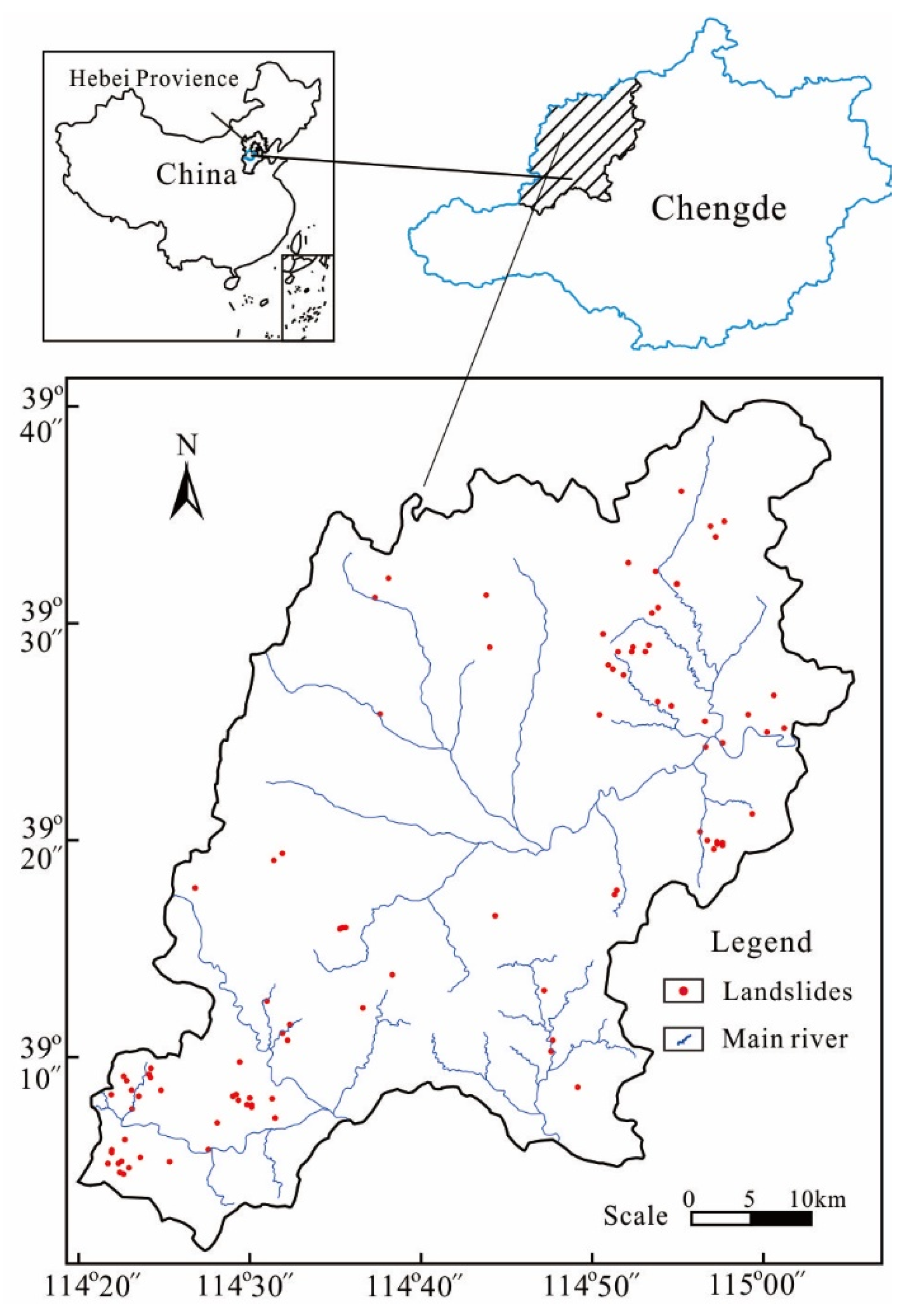
Laiyuan County is located in the northern Taihang Mountains in northwestern Hebei Province, China, as shown in Figure 1. The study area has a longitude of 114°20′30″–115°04′54″ and a latitude of 39°01′38″–39°40′36″, covering an area of approximately 2448 km2, as shown in Figure 1. Its terrain is higher in the northwest and lower in the southeast. The average elevation is approximately 1000 m above sea level, with isolated peaks of up to 2140 m. The study area has a semi-arid temperate continental monsoon climate, with an average annual rainfall of approximately 560 mm (according to the data from 2005 to 2020). The rainy season typically lasts from July to September, and it accounts for more than 70% of the total yearly amount of annual rainfall.
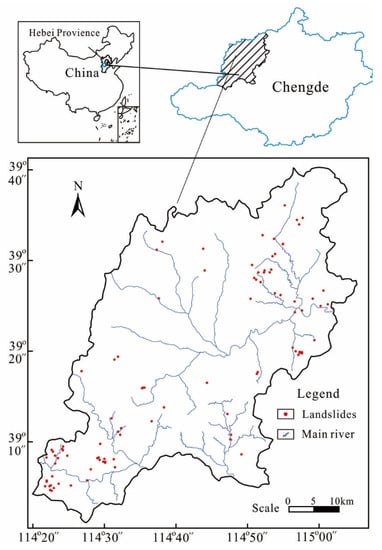
Figure 1.
The illustration of the study area.
The Archean age consists of amphibolite and granite gneiss. The lithology of the Proterozoic age is mainly comprised of dolomite and sandstone. The rocks of Cambrian and Ordovician systems are limestone, shale, and dolomite. The Jurassic geological formations mainly consist of sandstone, conglomerate, andesite, and tuff. The sedimentary rocks of Quaternary mainly are deposited near the river valley in the county. In general, the stratigraphic lithology of the study area is mainly composed of dolomite, limestone, granite gneiss, and intrusive granite. The geological structure of the study area is complex, and the faults are well developed.
Laiyuan County is a region particularly prone to landslides because of its complex geological environment, frequent rainstorms, and intense human activities. For instance, heavy rainfall hit the study area on 21 July 2012. The average and maximum precipitation reached more than 160 mm and 370 mm, respectively. In addition, a severe landslide occurred in the south of the county, resulting in land cover degradation and socio-economic damage. Due to urbanization, road and highway construction, and economic development, it is crucial to delineate LSM for the study area.
2.2. Data Acquisition
2.2.1. Landslide Inventory
To identify areas prone to landslides using machine learning-based methods, the historical data of landslide occurrences were taken as a vital piece of information. Overall, a total of 94 landslides, including hidden dangerous points, were obtained from multiple field investigations and historical records from 2006 to 2020. The types of landslide activities were small-scale based on the field monitoring data. Figure 1 shows the locations of landslides in detail. In this study, a pixel in the center of each landslide area was selected as a landslide location. Meanwhile, non-landslide locations with the same scale were randomly selected from areas free of landslides. For the non-landslide locations, the peripheral zones of historical landslides were selected as the main selection areas. Finally, landslide and non-landslide points were randomly split into two datasets; namely, approximately 70% of the locations (65 landslides and 65 non-landslides) were incorporated into training data, while the remaining locations were used for the model validation. This random portion of data has been recommended in the LSM-related literature [6,13,15,16,23].
2.2.2. Influencing Factors
Selecting suitable condition factors for LSM is a crucial step in this study. There has been no unique standard for selecting these factors due to their complex nature. Based on the previous research, historical landslide mechanisms, and availability of data in the study area [7,12,15,21,29], a total of 12 landslide-related factors were selected: elevation, slope, aspect, curvature, topographic wetness index (TWI), rainfall, distance to rivers, distance to faults, lithology, normalized difference vegetation index (NDVI), roads, and land use. All factors were converted into a thematic map with a grid size of 30 m × 30 m. Moreover, the continuous data on elevation, slope, curvature, TWI, rainfall, rivers, faults, NDVI, and roads were further classified into five categories using the natural break classification method. The rest of the factors (i.e., aspect, lithology, and land use) were classified into specific discrete subclasses.
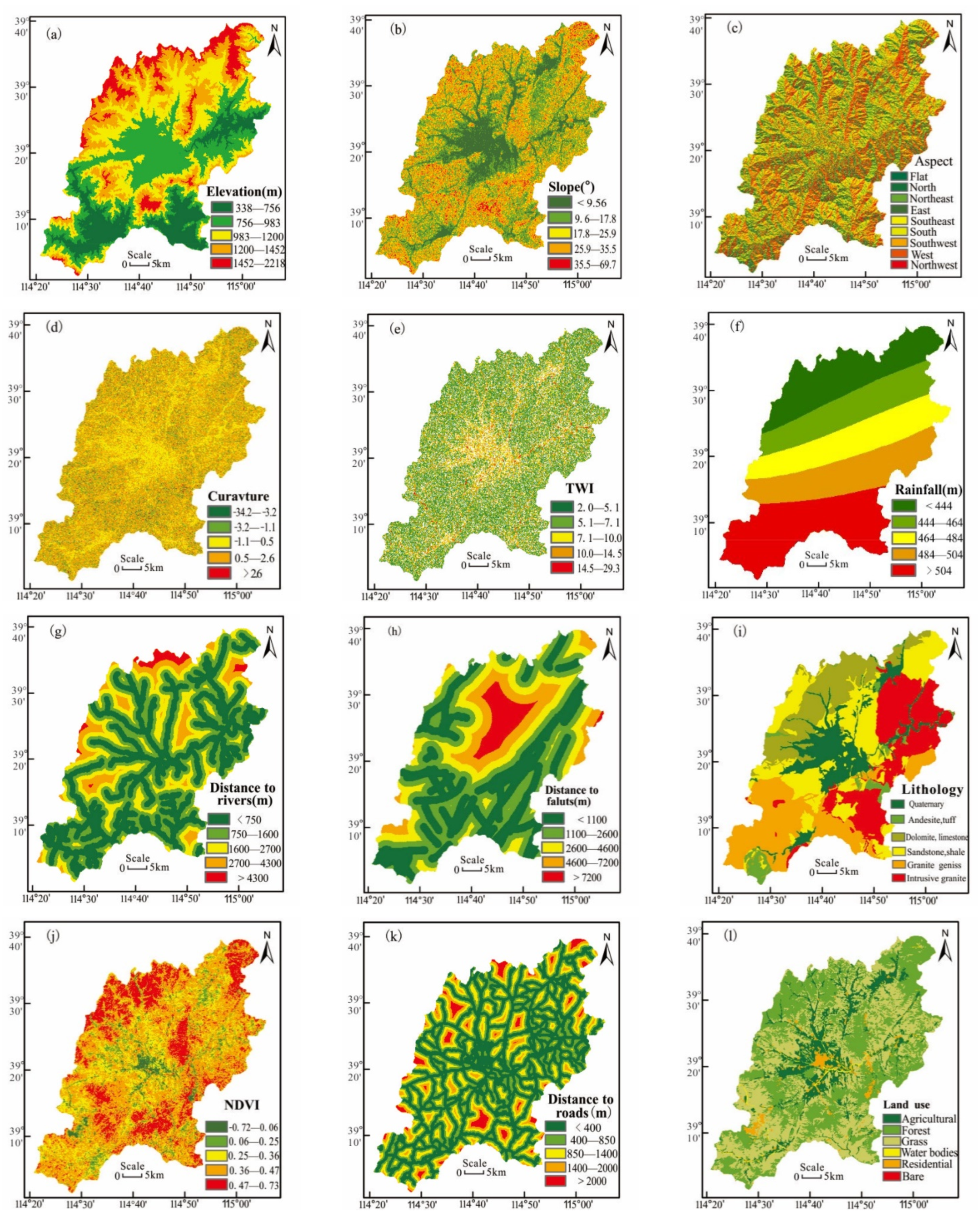
Elevation is an important factor that influences the local climate, vegetation, and availability of potential energy [30,31]. High elevation can easily induce landslides. In the study area, elevation ranged from 800 m to 2,200 m, as shown in Figure 2a.
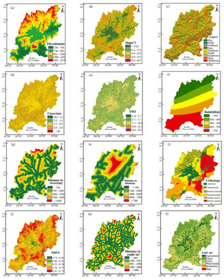
Figure 2.
The landslide conditioning factors: (a) elevation, (b) slope, (c) aspect, (d) curvature, (e) TWI, (f) rainfall, (g) distance to rivers, (h) distance to faults, (i) lithology, (j) NDVI, (k) distance to roads, and (l) land use.
The slope also plays a significant role in the analysis of landslide susceptibility. Related research has indicated that the possibility of landslides first increases with the slope angle up to a threshold value and then decreases [32]. In this study, the slope angle was divided into five classes, as shown in Figure 2b. Furthermore, the aspect or the direction of a slope defines the amount of water present on the slopes. Therefore, nine slope categories were identified: flat, north, northeast, east, southeast, south, southwest, west, and northwest, as shown in Figure 2c.
Moreover, the curvature is a factor that influences the acceleration and deceleration of the flow, thereby inducing landslides to a certain extent. Figure 2d shows the five curvature categories of the entire study area. The TWI was defined as a theoretical measure of flow accumulation and soil moisture at any point within a basin, which usually has a strong correlation with soil moisture [3,21]. The TWI values of the study area are shown in Figure 2e, and they were calculated by:
where α is the upslope area, and β is the slope in degrees.
The elevation, slope angle, aspect, curvature, and TWI were extracted by a digital elevation model (DEM) with a 30 m × 30 m resolution derived from a geospatial data cloud.
Rainfall, which is a vital external factor, alters the soil’s moisture content, raising interstitial pore water pressure and seepage pressure [12,23]. It is one of the most important induction factors for landslides. This study integrated the average annual precipitation data from 2005 to 2018 from eight rainfall gauge stations. Furthermore, the rainfall was mapped using the kriging method, as shown in Figure 2f.
The distance to a river was selected as an influencing factor since it can affect the influence of the hydrological environment on the development of landslides. Namely, areas close to rivers are prone to erosion, which may result in landslides. The locations of rivers were obtained from the topographic map having a scale of 1:50,000 in the GIS environment. The distance to rivers was measured using the spatial distance analysis tool in the GIS software, that is, the Euclidean distance tool, as shown in Figure 2g.
Faults reduce the integrity and strength of the rock formation, which plays an essential role in reducing slope stability [26]. Many studies indicated that areas close to faults are prone to landslides. The distance to faults was measured based on a buffer zone created by the Euclidean distance tool, as shown in Figure 2h.
In addition, lithology was considered an important indicator that affects the weather and mechanical characteristics of rocks [1,15]. As mentioned above, the lithology of the study area mainly comprised six geological formations, as shown in Figure 2i. The location and information on faults and lithological units were extracted from the national geological maps having a scale of 1:50,000.
The NDVI can reflect the impact of human activities and vegetation coverage rate on the occurrence of landslides [5]. The NVDI values were obtained from satellite images captured by Landsat 8 in 2018 using the red and near-infrared reflectance values, as shown in Figure 2j.
Due to its destructive nature, the construction of roads can negatively affect slope stability [14]. Thus, the distance to roads was taken as a crucial human factor in this research [27]. The information on roads was extracted from a topographic map having a scale of 1:50,000. The Euclidean distance tool in GIS was used to create a map with distances to roads, as shown in Figure 2k.
Lastly, the land use and cover also indicate the influence of human activities on the development of landslides. The map of land use from 2018 was derived from the Resources and Environment Data Cloud Platform, and the land in the study area was classified into five categories: agricultural land, forest, grass, water bodies, and bare land, as displayed in Figure 2l.
2.3. Proposed Method
This study includes five stages for predicting LSM: (1) collecting equal numbers of landslide and non-landslide locations; (2) determining and normalizing the factors that directly or indirectly influence the occurrence of landslides; (3) analyzing the correlation and multicollinearity of selected factors; (4) delineating the area prone to landslides using the RF, AB, GBDT, and XGBoost models; (5) validating and comparing these models using several performance metrics. The ensemble models were implemented in the Python 3.7 environment. To view the official home of the Python programming language through https://www.python.org/. Meanwhile, the code related to models in this work is modified based on an open source Python library scikit-learn package (https://github.com/scikit-learn/scikit-learn, accessed on 26 April 2022). The 10-fold cross-validation and trial-and-error methods were used to determine the optimal parameters. A detailed flowchart of the proposed method is shown in Figure 3.
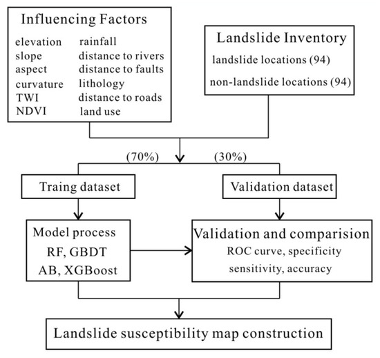
Figure 3.
The flowchart of the proposed method.
2.3.1. RF Method
Bagging algorithms, which are ensemble machine learning-based algorithms, have been proven to be a useful technique in building susceptibility models. The RF is a typical bagging algorithm for ensemble models and was developed by Breiman (2001) as a combination of decision trees [33,34]. In addition, the bootstrap sampling technique with replacement has often been performed to create several decision trees consisting of different subsamples of datasets and features [35]. The unselected variables or data are often called out-of-bag samples. Each decision tree is trained with independent datasets. Based on these datasets, the prediction and validation errors are calculated. The bootstrapping technique combined with the bagging algorithm helps the RF model avoid the overfitting problem. The main advantage of the RF is that it can reduce the variance of the base algorithm.
The performance of the RF depends on two parameters, the number of trees and the number of variables in each tree [33,36]. The RF algorithm uses the Gini impurity as a measure for the best split selection. The number of trees and variables in this study were selected based on the previous research [34,36]. In addition, the 10-fold cross-validation scheme and the grid search method were used to obtain optimal numbers of trees and variables.
2.3.2. AB Method
Since it was introduced by Freund and Schapire in 1997, the AB has been known as an extremely effective adaptive boosting algorithm in machine learning [12]. In this algorithm, a sample is randomly selected from the original dataset with the same weights during the process of bagging. However, the AB algorithm uses the same set of training samples to train different weak classifiers, contrary to bagging [26]. The samples are given equal weights at the beginning of the training, but in the next iteration, the weights of corrected classified samples are reduced, while the weights of improper ones are increased [12]. The same dataset with updated weights is used to train the next weak learner. Different from the RF algorithm, the AB algorithm can address the weakness of classifiers to continuously improve the accuracy during the modeling process. Finally, class membership is decided when several weak learners are combined and weighed according to their performance [37].
2.3.3. GBDT Method
The GBDT method belongs to the class of ensemble learning methods that combine classification and regression trees with gradient boosting [23,38]. It is one of the most effective ensemble methods in the boosting family because it ensembles several weak learners to construct a stronger one. The parameters of a weak classifier are set to approximate the gradient direction of reducing residuals in each iteration [13]. When the number of iterations or the value error reaches the predefined value, the iteration process terminates. Similar to the AB method, the GBDT method iteratively constructs base learners by reweighting misclassified observations [39]. However, unlike the AB method, in the GBDT method, weak classifiers are mutually dependent and connected [35]. The weighted summations of weak classifiers are combined to obtain a strong classifier after multiple iterations. The obvious advantage of this method is its strong generalization ability to fit the real data distribution.
2.3.4. XGBoost Method
The XGBoost method was developed by Chen and Guestrin in 2016, and it represents the combination of the gradient boosting algorithm and decision tree models [40]. This relatively new tree-based boosting ensemble method has attracted great attention in the landslide field in recent years since it can be used for both classification and regression tasks [41]. The XGBoost method originates from the gradient tree boosting algorithm but follows the principle of gradient boosting. The main objective of the XGBoost method is to combine several weak learners into a stronger, more accurate learner through multiple iterations, similar to the GBDT method. Due to its main idea to fit decision trees from the previous trees on residuals instead of outcomes, the XGBoost has been regarded as an improved model in comparison to regular gradient boosting. Similarly, the XGBoost algorithm has been considered a powerful approach to overcoming the overfitting problem not only by random subsampling but also by regularizing the objective function [36,41]. The main advantages of the method are its well-documented speed and accuracy. To obtain several hyperparameters, in this study, the learning rate was set to 0.05, and the maximum depth of trees was set to four.
2.4. Multicollinearity Test
The influencing factors were checked for multicollinearities to ensure the independence of two or more of them. The correlation analysis has shown that a relationship between two or more of the input variables may cause deviations. Based on the related research, the variance inflation factor (VIF) and tolerance (TOL) have been the most widely used indicators in geoscience, and they are defined by Equation (2) [3,23,28]. If a VIF value is larger than 10 or a TOL value is smaller than 0.1, the corresponding factors are multicollinear and must be removed from the experiment.
In Equation (2), Rj2 is the R-squared value of regression obtained by regressing a parameter j on all of the other parameters.
2.5. Model Validation and Comparison
Validation is key when evaluating the efficiency, applicability, and scientific significance of models [4]. The receiver operating characteristic curve (ROC) is obtained by plotting the true positive rate against the false-positive rate at various threshold settings [32,42]. The area under the receiver operating characteristic curve (AUC) has been a standard tool for evaluating and assessing model performance. The AUC value ranging from 0.5 to 1.0 can be expressed in five degrees: poor (<0.6), average (0.6–0.7), good (0.7–0.8), very good (0.8–0.9), and excellent (>0.9) [13].
In addition, this study used three statistical metrics, sensitivity, specificity, and accuracy, to validate the ensemble models. These validation metrics have been extensively used in the field of machine learning. The sensitivity, specificity, and accuracy were respectively calculated by [21]:
where TP (true positive) and TN (true negative) represent the numbers of correctly classified landslide and non-landslide pixels, respectively; FN (false negative) and FP (false positive) are the numbers of incorrectly classified landslide and non-landslide locations, respectively.
3. Results
3.1. Factor Selection
Factor selection is an important step in a susceptibility model. The possibility of multicollinearity between the 12 selected conditioning factors was analyzed using the TOL and VIF parameters. As shown in Table 1, elevation had the highest VIF value (2.384) but the lowest TOL value (0.419). In general, the VIF value was less than 10, while TOL was larger than 0.2, indicating that there were no significant correlations between the influencing factors [3,16,23]. Therefore, the 12 conditioning factors were in the same range of collinearity and reasonably applied to the developed model.

Table 1.
Multicollinearity results of the influencing factors.
3.2. Model Performance and Comparison
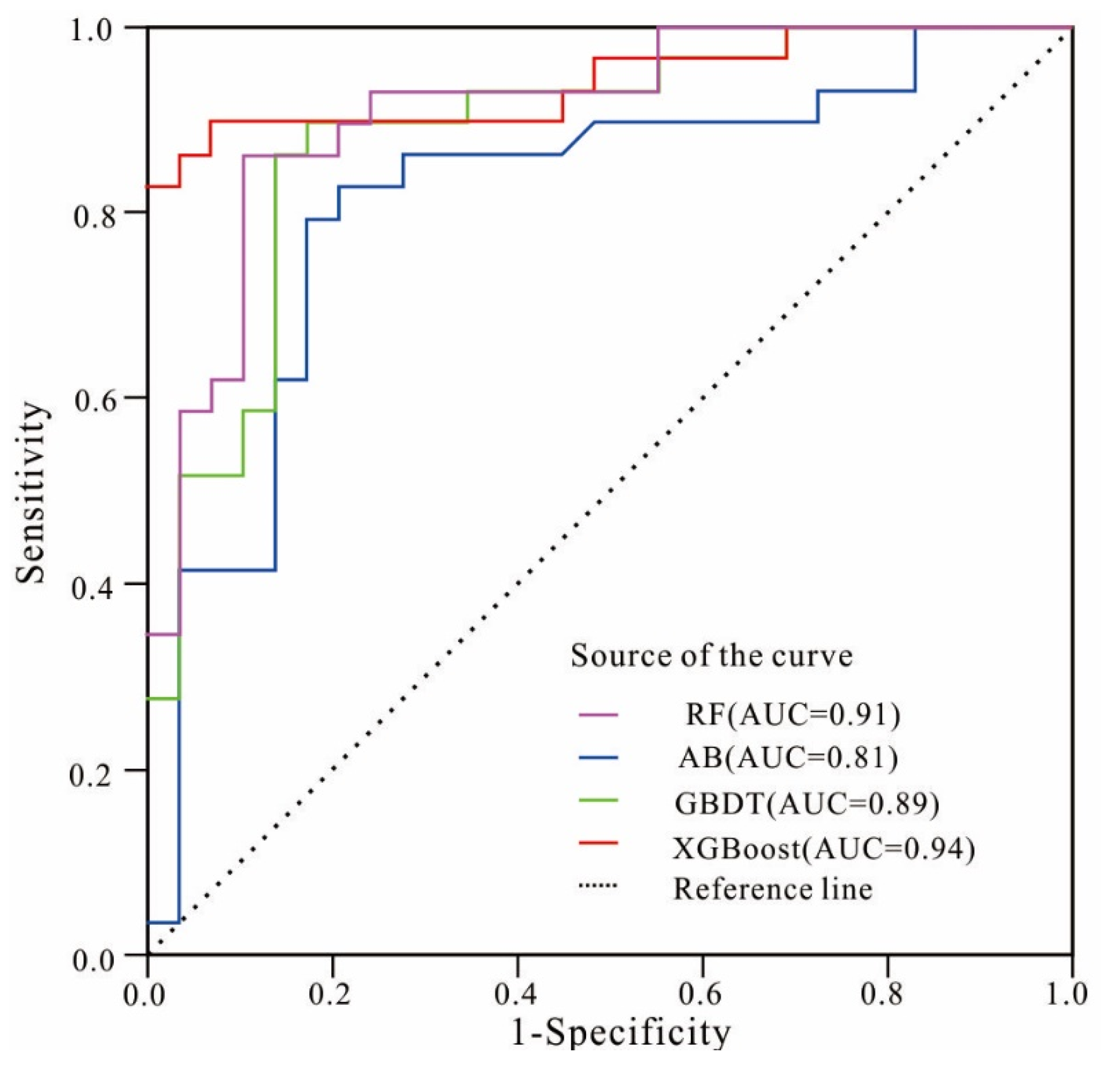
First, the ROC curve was used to validate and compare the accuracy of the RF, AB, GBDT, and XGBoost models, as shown in Figure 3. The performances of the models were evaluated using three statistic metrics (sensitivity, specificity, and accuracy), as presented in Table 2.
Table 2.
The performance results of the four models.
As presented in Figure 4, the AUC value was higher than 0.8, indicating that the four models were efficient in predicting the LSM. Among the four models, the XGBoost model (AUC = 0.94) performed the best; followed by the RF (AUC = 0.91), GBDT (AUC = 0.89), and AB (AUC = 0.81) models. In general, the AUC values of the XGBoost and RF models were excellent, while those of the GBDT and AB models were good.
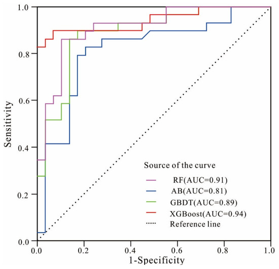
Figure 4.
The ROC curves of the four models.
According to the results in Table 2, the results of the three statistical metrics were similar to the ROC results. In terms of sensitivity and specificity, the XGBoost model proved to be the best fit, achieving a sensitivity of 92.86 and specificity of 90.00; it was followed by the RF model, which has a sensitivity of 89.29 and specificity of 86.67, the GBDT model, with a sensitivity of 86.21 and specificity of 86.21, and the AB model, which has a sensitivity of 82.14 and specificity of 86.03. Similarly, the XGBoost model had the highest accuracy of 91.38, followed by the RF model with an accuracy of 87.93, the GBDT model whose accuracy was 86.21, and the AB model that has the lowest accuracy of 81.03. Thus, the XGBoost and RF models performed significantly better than the GBDT and AB models.
The results indicated that the XGBoost model had the best performance and prediction capabilities in terms of AUC and statistic metrics. The RF model performed slightly better than the GBDT model, while the AB model had the lowest accuracy among the four models.
3.3. Landslide Susceptibility Mapping
Using the natural breaks method, the LSM results of the RF, AB, GBDT, and XGBoost models were classified into five categories: very low, low, moderate, high, and very high. Figure 5 shows the percentage of the five categories of the four models. A detailed distribution of the results of the four models is presented in Figure 6.
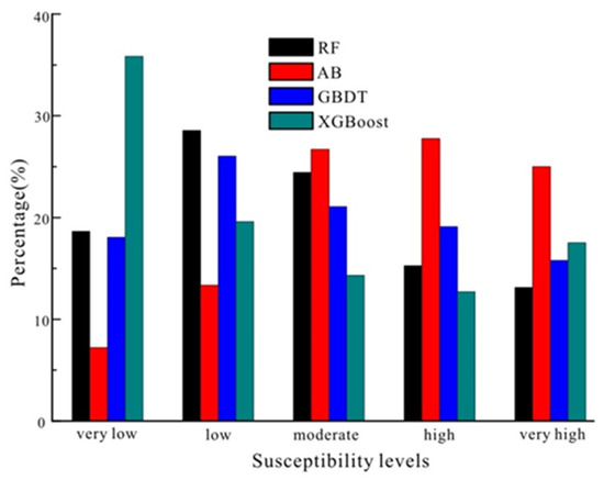
Figure 5.
The area percentage of landslide susceptibility.
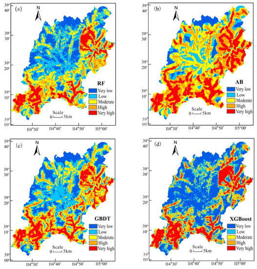
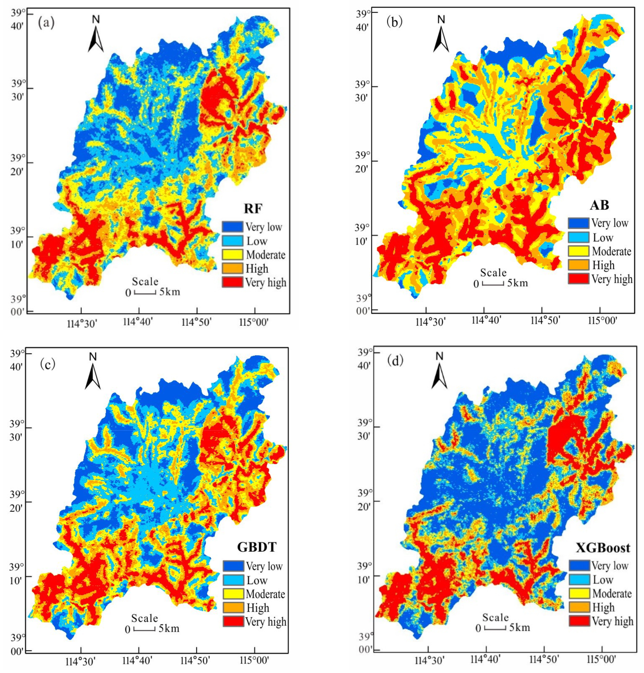
Figure 6.
The result of the ensemble models: (a) the RF model, (b) the AB model, (c) the GBDT model, and (d) the XGBoost model.
As shown in Figure 5, the landslide-prone property results of the four ensemble models showed certain differences. The RF, AB, GBDT, and XGBoost models had the highest percentage values for the low, high, low, and very low susceptible categories, respectively. For the RF model, the susceptibility of the total area ranging from very low to very high categories was 18.64%, 28.56%, 24.43%, 15.25%, and 13.12%. The percentage value of the AB model indicated that the areas of very low, low, moderate, high, and very high susceptibility accounted for 7.2%, 13.34%, 26.70%, 27.76%, and 25%, respectively. For the GBDT model, the areas of very low, low, moderate, high, and very high susceptibility accounted for 18.05%, 26.02%, 21.06%, 19.09%, and 15.78%, respectively. By using the XGBoost model, the areas ranging from the very low to the very high degree of susceptibility accounted for 35.84%, 19.58%, 14.33%, 12.71%, and 17.54%, respectively.
Specifically, the LSM results of the AB model were different from those of the other three models, as shown in Figure 5. The percentages of the highly susceptible areas (very high and high) accounted for approximately 30% of the total area for the maps predicted by the RF, GBDT, and XGBoost models, while those of the AB model accounted for more than 50%. The LSM result of the RF model was similar to that of the XGBoost model except for the very low category. The RF model classified 47% of the total area as a low susceptibility zone (very low and low), while 28.37% was classified as a zone of high susceptibility (very high and high). However, when the XGBoost model was used, 55.42% and 30.25% of the area were classified as the high and low susceptibility zones, respectively. In terms of the landslide susceptibility classification results (Figure 5), the XGBoost model performed similarly to the RF model.
As shown in Figure 6, the distribution results of areas prone to very high and high susceptibility predicted by the RF model coincided well with those predicted by the XGBoost model and were followed by the GBDT model. However, the LSM predicted by the AB model differed from those of the other models. Based on the distribution of landslide locations, most of the historical landslide records were located in areas with high susceptibility, as predicted by the XGBoost and RF models. Concerning the distribution of the landslide and non-landslide locations (Figure 1), the highest performance was achieved by the XGBoost model, followed by the RF, GB, and AB models, as shown in Figure 6.
As mentioned above, the XGBoost model had the highest accuracy among the four models, so the distribution results of the landslide susceptibility classifications of the XGBoost model were further analyzed, as shown in Figure 6. The high and very high categories were mostly observed in the south and northeast of Laiyuan County. In particular, areas prone to high susceptibility sporadically emerged in the northwest, especially along rivers and roads. As mentioned before, rivers may influence the induction of landslides. Similarly, steep slopes intersected by roads may be prone to landslides as well. Therefore, it is expected that human activities will probably be the dominant factor in the occurrence of landslides in the future, which requires special attention. Accordingly, measures for geohazard prevention should be taken in such areas. Conversely, low susceptibility areas were mainly disturbed in the north and the middle of Laiyuan County, that is, in areas with low elevation, flat slopes, and less human activity.
4. Discussion
A reliable LSM is crucial to predicting spatial locations where landslides may occur. In recent years, a large number of machine learning-based methods have been successfully applied to LSM prediction. Moreover, a number of related studies have proven that an ensemble model can perform better than a single machine learning-based model [16,43]. However, the selection of the ensemble model is still a critical task in LSM prediction, especially because the application of advanced ensemble models has been limited. Each machine learning-based method has its advantages and disadvantages, making its performance vary in different areas [37,40]. Generally, there has been no universal standard for delineating LSM using ensemble models.
This study aims to compare the performance of the prevailing ensemble models to obtain accurate LSM. The RF model has been widely used in LSM prediction, while the advanced boosting models, including the AB, GBDT, and XGBoost models have drawn much attention in recent years [5,27,36,44]. However, the performances of these boosting algorithms in predicting LSM have rarely been compared. Therefore, the bagging algorithm model, the RF model, and three typical boosting algorithms, the AB, GBDT, and XGBoost models, were analyzed and compared in this study.
In terms of the ROC results, the AUC values of all four models were greater than 0.80, indicating that the four typical ensemble models performed well in predicting the landslide susceptibility. Moreover, the results of three statistic metrics, sensitivity, specificity, and accuracy, indicated that all models yielded good and reasonable results. These results are in agreement with the previous studies, which have pointed out that the tree-based ensemble algorithms can achieve better results than the other algorithms [14,25,35].
The RF method is a tree-based ensemble model, which has been commonly used to map LSM [35,40]. In this study, the RF model outperformed the other two boosting ensemble models, the AB and GBDT model. The results of this study are in agreement with most of the related studies. For instance, Pourghasemi and Rahmati (2018) [45] compared the RF model, boosted regression trees, and classification and regression trees for LSM and found that the RF model performed the best among all models. Moreover, He et al. (2021) [35] compared the performance of the RF, AB, and GBDT models in predicting the landslide susceptibility and found that the RF model performed better than the other models. However, the detailed comparisons made by Micheletti et al. (2014) [37], Pham et al. (2017) [12], Wu et al. (2020) [26], and Liang et al. (2021) [23] indicated that the AB and GBDT models had higher accuracy than the RF model. Thus, the RF model does not always perform better than the boosting ensemble models.
According to the obtained results, the XGBoost model achieved the best goodness-of-fit result, followed by the RF, GBDT, and AB models. These results indicate that the XGBoost model had higher accuracy than the typical bagging model. This result is in agreement with the results of Cao et al. (2020) [40], Rabby et al. (2020) [36], and Kavzoglu and Teke (2022) [43], which also indicated that the XGBoost model performed better than the RF model in geohazards susceptibility mapping. Unlike the RF model, the XGBoost model reduces error mainly by decreasing the bias rather than variance. In addition, the newly developed gradient boosting model also outperformed the other two boosting ensemble models due to high regularization [36,40,44]. The efficiency of the XGBoost model in assessing the geological hazard susceptibility map has been previously reported by Zhang et al. (2019) [46], Cao et al. (2020) [40], and Hussain et al. (2021) [47]. In general, the advanced ensemble model, the XGBoost model, has been explored in a few studies on LSM, and it has also shown promising results in this study.
5. Conclusions
An accurate prediction of the occurrence of landslides in the study area is imperative. The aim of this study is to compare the boosting and bagging ensemble models and apply them to the LSM. Four advanced and typical ensemble machine learning-based models are used in Laiyuan County, Hebei Province, China. A landslide inventory consisting of 94 landslide and 94 non-landslide locations is randomly divided into the training dataset, including 70% of the total data, and the test set, including the remaining 30% of the total data. In addition, 12 dependent influencing factors were selected and prepared in the GIS environment after multicollinearity analysis.
The ROC results indicate that the four ensemble models (RF, AB, GBDT, and XGBoost models) are all suitable for predicting the LSM, having an AUC of more than 0.8. In the comparison test, the XGBoost model achieved the highest statistic metrics: a sensitivity of 92.86, specificity of 90.00, accuracy of 91.38, and AUC of 0.94, and it was identified as the best ensemble model. It was followed by the RF model (sensitivity = 89.29, specificity = 86.67, accuracy = 87.93, and AUC = 0.91), the GBDT model (sensitivity = 86.21, specificity = 86.21, accuracy = 86.21, and AUC = 0.89), and AB (sensitivity = 82.14, specificity = 80.00, accuracy = 81.03, and AUC = 0.81). Therefore, the XGBoost model was identified as the best tree-based ensemble model for predicting the LSM. In addition, the RF model performed better than the AB and GBDT models due to its more accurate prediction capability, so it could also be seen as a promising tool for LSM prediction.
Using the natural breakpoint method, the LSM results of the four models are classified into five susceptibility categories: very low, low, moderate, high, and very high. The prediction results of areas prone to landslides show that there are certain differences in susceptibility zones between different algorithms. The AB model’s results differed from the other models’ results. The LSM results obtained by the highly accurate models, namely the XGBoost and RF models, had very similar spatial distribution patterns. According to the results, areas with high and very high susceptibility should be prioritized during the landslide prevention planning.
In general, all compared models have an acceptable level of prediction accuracy, but the XGBoost model has a superior performance compared to the other models, which makes it a promising ensemble model for LSM prediction.
The results presented in this paper could be used to reduce the risk of landslides and plan land usage. However, this study does not include further optimization (e.g., hyperparameters) but only the trial-and-error methods and grid search, which is its main limitation. Therefore, future research should focus on a more detailed comparison of the ensemble models for predicting the LSM.
Author Contributions
Conceptualization, A.W. and K.Y.; investigation, W.Z. and Y.L.; methodology, A.W. and K.Y.; resources, F.G.; software, F.D. and F.G.; validation, F.G. and W.Z.; visualization, W.Z. and Y.L.; writing—original draft, A.W.; writing—review and editing, K.Y. and F.D. All authors have read and agreed to the published version of the manuscript.
Funding
This research was funded by the S&T Program of Hebei (D2019403194 and E2021403001) and the Graduate Students Teaching Case of Hebei Province (KCJSZ2019090).
Institutional Review Board Statement
Not applicable.
Informed Consent Statement
Not applicable.
Data Availability Statement
Data are available on request from the corresponding author.
Conflicts of Interest
The authors declare no conflict of interest.
References
- Kavzoglu, T.; Sahin, E.K.; Colkesen, I. Landslide susceptibility mapping using GIS-based multi-criteria decision analysis, support vector machines, and logistic regression. Landslides 2014, 11, 425–439. [Google Scholar] [CrossRef]
- Martha, T.R.; van Westen, C.J.; Kerle, N.; Jetten, V.; Kumar, K.V. Landslide hazard and risk assessment using semi-automatically created landslide inventories. Geomorphology 2013, 184, 139–150. [Google Scholar] [CrossRef]
- Lee, J.H.; Sameen, M.I.; Pradhan, B.; Park, H.J. Modeling landslide susceptibility in data-scarce environments using optimized data mining and statistical methods. Geomorphology 2018, 303, 284–298. [Google Scholar] [CrossRef]
- Berhane, G.; Kebede, M.; Alfarrah, N. Landslide susceptibility mapping and rock slope stability assessment using frequency ratio and kinematic analysis in the mountains of Mgulat area, Northern Ethiopia. Bull. Eng. Geol. Environ. 2021, 80, 285–301. [Google Scholar] [CrossRef]
- Huang, F.; Ye, Z.; Jiang, S.H.; Huang, J.; Chang, Z.; Chen, J. Uncertainty study of landslide susceptibility prediction considering the different attribute interval numbers of environmental factors and different data-based models. Catena 2021, 202, 105250. [Google Scholar] [CrossRef]
- Wang, S.; Zhuang, J.; Zheng, J.; Fan, H.; Kong, J.; Zhan, J. Application of Bayesian hyperparameter optimized random forest and XGBoost model for landslide susceptibility mapping. Front. Earth Sci. 2021, 617. [Google Scholar] [CrossRef]
- Shirvani, Z. A holistic analysis for landslide susceptibility mapping applying geographic object-based random forest: A comparison between protected and non-protected forests. Remote Sens. 2020, 12, 434. [Google Scholar] [CrossRef] [Green Version]
- Aditian, A.; Kubota, T.; Shinohara, Y. Comparison of GIS-based landslide susceptibility models using frequency ratio, logistic regression, and artificial neural network in a tertiary region of Ambon, Indonesia. Geomorphology 2018, 318, 101–111. [Google Scholar] [CrossRef]
- Baharvand, S.; Rahnamarad, J.; Soori, S.; Saadatkhah, N. Landslide susceptibility zoning in a catchment of Zagros Mountains using fuzzy logic and GIS. Environ. Earth Sci. 2020, 79, 204. [Google Scholar] [CrossRef]
- Reichenbach, P.; Rossi, M.; Malamud, B.D.; Mihir, M.; Guzzetti, F. A review of statistically-based landslide susceptibility models. Earth-Sci. Rev. 2018, 180, 60–91. [Google Scholar] [CrossRef]
- Kayastha, P.; Dhital, M.R.; De Smedt, F. Application of the analytical hierarchy process (AHP) for landslide susceptibility mapping: A case study from the Tinau watershed, west Nepal. Comput. Geosci. 2013, 52, 398–408. [Google Scholar] [CrossRef]
- Pham, B.T.; Bui, D.T.; Prakash, I.; Dholakia, M.B. Hybrid integration of multilayer perceptron neural networks and machine learning ensembles for landslide susceptibility assessment at Himalayan area (India) using GIS. Catena 2017, 149, 52–63. [Google Scholar] [CrossRef]
- Wang, Y.; Feng, L.; Li, S.; Ren, F.; Du, Q. A hybrid model considering spatial heterogeneity for landslide susceptibility mapping in Zhejiang Province, China. Catena 2020, 188, 104425. [Google Scholar] [CrossRef]
- Akinci, H.; Zeybek, M. Comparing classical statistic and machine learning models in landslide susceptibility mapping in Ardanuc (Artvin), Turkey. Nat. Hazards 2021, 108, 1515–1543. [Google Scholar] [CrossRef]
- Farooq, S.; Akram, M.S. Landslide susceptibility mapping using information value method in Jhelum Valley of the Himalayas. Arab. J. Geosci. 2021, 14, 824. [Google Scholar] [CrossRef]
- Dou, J.; Yunus, A.P.; Bui, D.T.; Merghadi, A.; Sahana, M.; Zhu, Z.; Chen, C.; Han, Z.; Pham, B.T. Improved landslide assessment using support vector machine with bagging, boosting, and stacking ensemble machine learning framework in a mountainous watershed, Japan. Landslides 2020, 17, 641–658. [Google Scholar] [CrossRef]
- Habumugisha, J.M.; Chen, N.; Rahman, M.; Islam, M.M.; Ahmad, H.; Elbeltagi, A.; Sharma, G.; Liza, S.N.; Dewan, A. Landslide susceptibility mapping with deep learning algorithms. Sustainability 2022, 14, 1734. [Google Scholar] [CrossRef]
- Jennifer, J.J.; Saravanan, S. Artificial neural network and sensitivity analysis in the landslide susceptibility mapping of Idukki district, India. Geocarto Int. 2021, 1–23. [Google Scholar] [CrossRef]
- Harirchian, E.; Hosseini, S.E.A.; Jadhav, K.; Kumari, V.; Rasulzade, S.; Işık, E.; Wasif, M.; Lahmer, T. A review on application of soft computing techniques for the rapid visual safety evaluation and damage classification of existing buildings. J. Build. Eng. 2021, 43, 102536. [Google Scholar] [CrossRef]
- Goetz, J.N.; Brenning, A.; Petschko, H.; Leopold, P. Evaluating machine learning and statistical prediction techniques for landslide susceptibility modeling. Comput. Geosci. 2015, 81, 1–11. [Google Scholar] [CrossRef]
- Bragagnolo, L.; da Silva, R.V.; Grzybowski, J.M.V. Artificial neural network ensembles applied to the mapping of landslide susceptibility. Catena 2020, 184, 104240. [Google Scholar] [CrossRef]
- Li, B.; Li, J. Methods for landslide detection based on lightweight YOLOv4 convolutional neural network. Earth Sci. Inform. 2022, 1–11. [Google Scholar] [CrossRef]
- Liang, Z.; Wang, C.; Khan, K.U.J. Application and comparison of different ensemble learning machines combining with a novel sampling strategy for shallow landslide susceptibility mapping. Stoch. Environ. Res. Risk A 2021, 35, 1243–1256. [Google Scholar] [CrossRef]
- Sahin, E.K. Comparative analysis of gradient boosting algorithms for landslide susceptibility mapping. Geocarto Int. 2020, 1–25. [Google Scholar] [CrossRef]
- Merghadi, A.; Yunus, A.P.; Dou, J.; Whiteley, J.; ThaiPham, B.; Bui, D.T.; Avtar, R.; Abderrahmane, B. Machine learning methods for landslide susceptibility studies: A comparative overview of algorithm performance. Earth-Sci. Rev. 2020, 207, 103225. [Google Scholar] [CrossRef]
- Wu, Y.; Ke, Y.; Chen, Z.; Liang, S.; Zhao, H.; Hong, H. Application of alternating decision tree with AdaBoost and bagging ensembles for landslide susceptibility mapping. Catena 2020, 187, 104396. [Google Scholar] [CrossRef]
- Al-Najjar, H.A.; Pradhan, B.; Kalantar, B.; Sameen, M.I.; Santosh, M.; Alamri, A. Landslide susceptibility modeling: An integrated novel method based on machine learning feature transformation. Remote Sens. 2021, 13, 3281. [Google Scholar] [CrossRef]
- Pham, Q.B.; Achour, Y.; Ali, S.A.; Parvin, F.; Vojtek, M.; Vojteková, J.; Al-Ansari, N.; Achu, A.L.; Costache, R.; Khedher, K.M.; et al. A comparison among fuzzy multi-criteria decision making, bivariate, multivariate and machine learning models in landslide susceptibility mapping. Geomat. Nat. Hazards Risk 2021, 12, 1741–1777. [Google Scholar] [CrossRef]
- Meena, S.R.; Soares, L.P.; Grohmann, C.H.; van Westen, C.; Bhuyan, K.; Singh, R.P.; Floris, M.; Catani, F. Landslide detection in the Himalayas using machine learning algorithms and U-Net. Landslides 2022, 19, 1209–1229. [Google Scholar] [CrossRef]
- Vasu, N.N.; Lee, S.R. A hybrid feature selection algorithm integrating an extreme learning machine for landslide susceptibility modeling of Mt. Woomyeon, South Korea. Geomorphology 2016, 263, 50–70. [Google Scholar] [CrossRef]
- Park, H.J.; Kim, K.M.; Hwang, I.T.; Lee, J.H. Regional landslide hazard assessment using extreme value analysis and a probabilistic physically based approach. Sustainability 2022, 14, 2628. [Google Scholar] [CrossRef]
- Kouhartsiouk, D.; Perdikou, S. The application of DInSAR and Bayesian statistics for the assessment of landslide susceptibility. Nat. Hazards 2021, 105, 2957–2985. [Google Scholar] [CrossRef]
- Breiman, L. Random forests. Mach. Learn. 2001, 45, 5–32. [Google Scholar] [CrossRef] [Green Version]
- Youssef, A.M.; Pourghasemi, H.R.; Pourtaghi, Z.S.; Al-Katheeri, M.M. Landslide susceptibility mapping using random forest, boosted regression tree, classification and regression tree, and general linear models and comparison of their performance at Wadi Tayyah Basin, Asir Region, Saudi Arabia. Landslides 2016, 13, 839–856. [Google Scholar] [CrossRef]
- He, Q.; Jiang, Z.; Wang, M.; Liu, K. Landslide and wildfire susceptibility assessment in Southeast Asia using ensemble machine learning methods. Remote Sens. 2021, 13, 1572. [Google Scholar] [CrossRef]
- Rabby, Y.W.; Hossain, M.B.; Abedin, J. Landslide susceptibility mapping in three Upazilas of Rangamati hill district Bangladesh: Application and comparison of GIS-based machine learning methods. Geocarto Int. 2020, 1–27. [Google Scholar] [CrossRef]
- Micheletti, N.; Foresti, L.; Robert, S.; Leuenberger, M.; Pedrazzini, A.; Jaboyedoff, M.; Kanevski, M. Machine learning feature selection methods for landslide susceptibility mapping. Math. Geosci. 2014, 46, 33–57. [Google Scholar] [CrossRef] [Green Version]
- Friedman, J.H. Greedy function approximation: A gradient boosting machine. Ann. Stat. 2001, 29, 1189–1232. [Google Scholar] [CrossRef]
- Dev, V.A.; Eden, M.R. Formation lithology classification using scalable gradient boosted decision trees. Comput. Chem. Eng. 2019, 128, 392–404. [Google Scholar] [CrossRef]
- Cao, J.; Zhang, Z.; Du, J.; Zhang, L.; Song, Y.; Sun, G. Multi-geohazards susceptibility mapping based on machine learning—A case study in Jiuzhaigou, China. Nat. Hazards 2020, 102, 851–871. [Google Scholar] [CrossRef]
- Stanley, T.A.; Kirschbaum, D.B.; Sobieszczyk, S.; Jasinski, M.F.; Borak, J.S.; Slaughter, S.L. Building a landslide hazard indicator with machine learning and land surface models. Environ. Modell. Softw. 2020, 129, 104692. [Google Scholar] [CrossRef]
- Bradley, A.P. The use of the area under the ROC curve in the evaluation of machine learning algorithms. Pattern Recogn. 1997, 30, 1145–1159. [Google Scholar] [CrossRef] [Green Version]
- Kavzoglu, T.; Teke, A. Predictive Performances of ensemble machine learning algorithms in landslide susceptibility mapping using random forest, extreme gradient boosting (XGBoost) and natural gradient boosting (NGBoost). Arab. J. Sci. Eng. 2022, 1–19. [Google Scholar] [CrossRef]
- Pradhan, A.M.S.; Kim, Y.T. Rainfall-induced shallow landslide susceptibility mapping at two adjacent catchments using advanced machine learning algorithms. ISPRS Int. J. Geo-Inf. 2020, 9, 569. [Google Scholar] [CrossRef]
- Pourghasemi, H.R.; Rahmati, O. Prediction of the landslide susceptibility: Which algorithm, which precision? Catena 2018, 162, 177–192. [Google Scholar] [CrossRef]
- Zhang, Y.; Ge, T.; Tian, W.; Liou, Y.A. Debris flow susceptibility mapping using machine-learning techniques in Shigatse area, China. Remote Sens. 2019, 11, 2801. [Google Scholar] [CrossRef] [Green Version]
- Hussain, M.A.; Chen, Z.; Wang, R.; Shoaib, M. PS-InSAR-Based Validated Landslide Susceptibility Mapping along Karakorum Highway, Pakistan. Remote Sens. 2021, 13, 4129. [Google Scholar] [CrossRef]


Publisher’s Note: MDPI stays neutral with regard to jurisdictional claims in published maps and institutional affiliations. |
© 2022 by the authors. Licensee MDPI, Basel, Switzerland. This article is an open access article distributed under the terms and conditions of the Creative Commons Attribution (CC BY) license (https://creativecommons.org/licenses/by/4.0/).