Spatiotemporal Variability in Precipitation Extremes in the Jianghuai Region of China and the Analysis of Its Circulation Features

Abstract

In the context of global warming, changes in extreme-precipitation events are becoming increasingly complex, and investigating the spatial and temporal variation characteristics of extreme precipitation is extremely important for scientific water-resource planning, preventing new climate risks and maintaining ecosystem balances. Based on the daily precipitation from 1960–2017 at 15 meteorological stations in the Jianghuai region, the extreme-precipitation indices were calculated. The variations in 12 extreme-precipitation indices were detected by using the Mann–Kendall test in the Jianghuai region. The periodicity of indices was examined by wavelet analysis detecting significant time sections. Through the cross wavelet transform and wavelet coherence analyses, the nonlinear connections between extreme precipitation and atmospheric circulation were explored. The results indicate significant increasing trends in the max one-day precipitation amount (Rx1day), extreme wet days (R99p), and simple precipitation intensity index (SDII). The intensity of extreme precipitation increased significantly. The variation in extreme precipitation showed different trends in different regions, with a greater likelihood of increasing extreme-precipitation intensity and frequency in the southern region compared to the central and northern regions. The period of most oscillations of the indices tend toward be on a time scale of 2–4 years and are in the 1990s. The number of heavy precipitation days (R10 mm) and number of very heavy precipitation days (R20 mm) had, mainly, periods of 5.84 years. Additionally, there were significant resonance periods between the extreme-precipitation indices and the atmospheric circulation index; however, there were obvious differences in time domains. The North Atlantic Oscillation (NAO) and East Asian summer monsoon (EASM) had the most significant effect on the duration of extreme precipitation; Atlantic Oscillation (AO) and EASM had the most significant influence on the extreme-precipitation intensity. The results of the study can provide a scientific basis for water-resource management and disaster prevention and control in the Jianghuai region.

1. Introduction

Global and regional warming due to increased atmospheric concentrations of greenhouse gases has accelerated the hydrological cycle process and caused serious impacts on agricultural production and the ecological environment. Ground-based observations show that the global mean temperature increased by 0.74 °C in the 20th century, with a significant increasing trend, especially after 1950 [1]. The International Panel on Climate Change’s Sixth Assessment Report states that the global temperature increase is expected to reach 1.5 °C in the next 20 years [2]. A rise in temperature leads to an increase in atmospheric water-vapor content [3,4], which changes barometric pressure, wind speed, and saturated water-vapor pressure [5], thereby affecting rainfall characteristics [6]. Under these conditions, as the global hydrological cycle accelerates, extreme-precipitation events occur frequently, which trigger severe flooding, soil erosion, and other natural disasters [7,8,9], posing a great threat to agricultural production, ecosystems, and social development [10,11]. Therefore, it is important to identify the spatial and temporal characteristics of extreme precipitation and its influencing factors for disaster prevention and mitigation and prediction of possible future climate-based risks.

Globally, precipitation variability has been characterized by widespread and significant [12,13]. As indicated by the Clausius–Clapeyron equation, precipitation increases sharply under global warming conditions [14,15]. Through climate model simulation and observational surveys, many studies have found that precipitation extremes increase with global warming [16,17]. However, changes in total precipitation and extremes vary significantly among regions due to topography and local microclimates [18]. As reported by Gu et al. [19], while the trend of global mean precipitation was not significant, precipitation increased in the tropics and decreased in the mid-latitudes of the Northern Hemisphere. Yang et al. [20] found an increasing trend in extreme precipitation in northern and southern Canada, while the central region showed a downward trend during 1950–2012. Due to the influence of human activities, since 1900, extreme-precipitation events in the central part of the US Gulf Coast, for a given return time, have become more frequent [21]. In some parts of Germany, extreme precipitation has shown a decreasing trend, while in southern and western Africa, extreme-precipitation changes have not been clearly characterized [22]. In most parts of Central Asia, extreme-precipitation events have become more frequent [23]. Fujibe et al. [24] investigated extreme-precipitation intensity changes in Japan and found that strong precipitation increased and weak precipitation decreased. In China, the frequency and intensity of extreme-precipitation events have been increasing in the last 50 years due to climate change, and there are significant spatial differences [25]. Yue et al. [26] pointed out that more than half of the meteorological stations in China showed an increasing trend in both the intensity and frequency of extreme precipitation. Extreme precipitation showed a significant increasing trend in the Yangtze River Basin, and southwestern and southern China, while it showed a decreasing trend in northeastern and northern China [27]. Researchers have also predicted future changes in extreme precipitation. Under global climate model simulations and the RCP8.5 scenario, an increase in runoff due to a surge in precipitation is projected for the Sierra Nevada in California [28]. Similarly, extreme-precipitation events will occur frequently in the Nile River Basin [29], northeastern Spain [30], Sicily, Italy [31] and China [32].

Atmospheric circulation is closely related to extreme precipitation. Hatzaki and Wu [33] found that extreme precipitation in southeastern Europe is highly correlated with SST anomalies in the tropical North Atlantic. In the Mediterranean Sea, extreme winter precipitation is mainly influenced by the North Atlantic Oscillation (NAO) and the Arctic Oscillation (AO) [34]. Yang et al. [20] found changes in extreme precipitation to have strong teleconnections with the Pacific Decadal Oscillation (PDO) and North Atlantic Oscillation, etc. In the central part of the US Gulf Coast, the changes in extreme-precipitation events were related to El Niño [21]. In most parts of Central Asia, extreme precipitation is likely to be related to the Siberian High and Tibetan Plateau Index_B atmospheric circulation factors [23]. In China, there is a significant positive correlation between the AO and the frequency of extreme-precipitation events in China in January–February [35]. When the Pacific Interdecadal Oscillation (PIO) and El Niño are in a warm phase, the frequency of extreme-precipitation events increases in western and central China, while the opposite is true in northeastern China [36]. In addition, the relationship between atmospheric rivers and extreme precipitation is also very close [37,38,39], and the total contribution rate of atmospheric rivers to the Meiyu in the Yangtze and Huaihe River Basin reaches more than 50% [40]. However, most of the studies mainly focus on the linear relationship between extreme precipitation and atmospheric circulation [41,42]. The response between extreme precipitation and atmospheric circulation is often asymmetrical and cannot be expressed linearly [43]. To analyze the relationship between atmospheric circulation factors and extreme precipitation, it is important to consider nonlinear and multiscale effects between them, and it is particularly important to explore the coupled oscillation relationship between atmospheric circulation and extreme precipitation.

The Jianghuai region is an important agricultural area in China; water resources are vital to agricultural production in the region and precipitation is one of the important sources of water resources in the region [44]. Due to the influence of climate warming, the intensity and frequency of precipitation in the region have changed, resulting in frequent flood and drought disasters, which are characterized by several occurrences a year, long disaster periods that often occur in consecutive seasons or years, and alternating floods and droughts [45]. In addition, the impact of human activities has changed the nature of the substratum, accelerated the water-cycle process, and further intensified the intensity of water and drought disasters. Changes in precipitation intensity and frequency affect the amount of available water resources and water-consumption processes in the Jianghuai region, and such temporal and spatial changes will have a significant impact on the spatial and temporal distribution and utilization of water resources and agricultural production.

Under the influence of global warming, the study of temporal and spatial variation patterns of extreme-precipitation indices will help clarify the relationship between the climate and the water cycle and can provide a scientific basis for water-resource management, the formulation of reasonable irrigation and drainage schemes and planting-structure adjustment in the region. Therefore, the main objectives of this study are to calculate extreme-precipitation indices in the Jianghuai region from 1960–2017 using daily precipitation data from meteorological stations, study the characteristics of temporal and spatial variations in extreme-precipitation indices and periodic variations, explore the drivers of extreme-precipitation variability and identify its main factors.

2. Data and Methods

2.1. Study Area

The Jianghuai region is located between the Yangtze River Basin and the Huaihe River Basin (29° N~35° N, 114° E~122° E), with a land area of approximately 31,000 km² (Figure 1). The study area has a subtropical monsoon climate with a warm and humid climate. The multiyear average precipitation is 1100 mm, the maximum precipitation is 1600 mm, the minimum precipitation is 584 mm, and 47% of the rainfall is concentrated from June to August. The multiyear average temperature is 14.8 °C, with a maximum of 39 °C and a minimum of −11 °C [46]. The multiyear average wind speed is between 3.2 and 3.5 m/s. Northerly winds prevail in winter, and southerly winds prevail in summer. The region is one of China’s major grain suppliers and is affected by monsoons and frequent droughts, floods, and flooding disasters, which seriously affect agricultural production.

2.2. Data Sources

The daily precipitation at 15 meteorological stations for the time series of 1960–2017 (

Table 1. Distribution of meteorological stations in the Jianghuai region.

Station Name	Latitude (°N)	Longitude (°E)	Elevation (m)
Xinyang	32.13	114.05	1145
Xuyi	32.98	118.52	408
Sheyang	33.77	120.25	20
Gushi	32.17	115.62	429
Shouxian	32.55	116.78	227
Chuxian	32.30	118.30	275
Gaoyou	32.80	119.45	54
Dongtai	32.87	120.32	43
Nantong	31.98	120.88	61
Luan	31.75	116.50	605
Huoshan	31.40	116.32	864
Tongcheng	31.07	116.95	854
Hefei	31.78	117.30	270
Chaohu	31.62	117.87	224
Anqing	30.53	117.05	198

) used in this study was obtained from the National Climate Centre of the China Meteorological Administration (CMA). The plausibility of the precipitation data was assessed by plotting the daily data for each station [47]. For missing data, the average of two adjacent stations was used for interpolation. The RClimDex software package (Version 2.15.2) was used to control the quality and test the homogeneity of the precipitation time-series data [48,49,50]. To investigate the influence of atmospheric circulation on extreme precipitation, we investigated the association of eight atmospheric circulation indices with extreme precipitation. Atlantic Oscillation (AO), Southern Oscillation Index (SOI), Oceanic Niño Index (ONI), and Western Pacific Index (WP) data were obtained from http://www.cpc.ncep.noaa.gov/ (accessed on 15 December 2021). The North Atlantic Oscillation (NAO), East Asian summer monsoon (EASM), South China Sea monsoon index (SCSMI) data were obtained from http://ljp.gcess.cn/dct/page/1 (accessed on 2 December 2021). Pacific Decadal Oscillation (PDO) data were obtained from http://www.esrl.noaa.gov/psd/data/correlation/pdo.data (accessed on 6 December 2021).

2.3. Methods

2.3.1. Extreme-Precipitation Indices

The extreme-precipitation indices used in this study included one-day, three-day, and five-day maximum precipitation amount (Rx1day, Rx3day, Rx5day), very wet days (R95p), extreme wet days (R99p), the simple precipitation intensity index (SDII), annual total wet-day precipitation (PRCPTOT), number of heavy precipitation days (R10 mm), number of very heavy precipitation days (R20 mm), number of extreme heavy precipitation days (R50 mm), number of consecutive dry days (CDD), and number of consecutive wet days (CWD). Among these indicators, one-day and three-day rainstorms are important design criteria in the technical specifications of Chinese farmland drainage engineering, and the rest are recommended by the ETCCDI (

Table 2. Definition of precipitation climate indices. Daily precipitation amount (RR).

Index	Indicator Name	Definition	Units
Rx1day	Max 1-day precipitation amount	Annual maximum 1-day precipitation amount	mm
Rx3day	Max 3-day precipitation amount	Annual maximum 3-day precipitation amount	mm
Rx5day	Max 5-day precipitation amount	Annual maximum 5-day precipitation amount	mm
R95p	Very wet days	Total annual precipitation from days with RR > 95th percentile	mm
R99p	Extreme wet days	Total annual precipitation from days with RR > 99th percentile	mm
SDII	Simple precipitation intensity index	The ratio of annual total wet-day precipitation to the number of wet days	mm/day
PRCPTOT	Annual total wet-day precipitation	Total annual precipitation from days with RR ≥ 1 mm	mm
R10 mm	Number of heavy precipitation days	Annual count of days with RR ≥ 10 mm	Days
R20 mm	Number of very heavy precipitation days	Annual count of days with RR ≥ 20 mm	Days
R50 mm	Number of extreme heavy precipitation days	Annual count of days with RR ≥ 50 mm	Days
CWD	Consecutive wet days	Maximum number of consecutive days with RR ≥ 1 mm	Days
CDD	Consecutive dry days	Maximum number of consecutive days with RR < 1 mm	Days

). In this study, the Rx3day was calculated by using self-programming in the MATLAB software. Other extreme-precipitation indicators were calculated for each site using the RClimDex software package.

2.3.2. Mann-Kendall Trend

The nonparametric Mann–Kendall (M-K) test has been widely applied in the study of hydrological change trends [51,52,53], and in this study, the Mann–Kendall test was used to analyze the trend of the series of extreme-precipitation indicators. The test statistic (S) is described by the following equation:

$$S={\displaystyle \sum _{k=1}^{n-1}{\displaystyle \sum _{j=k+1}^{n}Sgn(S_j-S_k)}}$$

(1)

where S_k and S_j are time-series data from k = 1, 2, …, n − 1, j = k + 1, …, n, S_j is greater than S_k, and n is the number of data points. Each S_k point is used as a reference point of S_j, and the results are recorded as Sgn(S_j − S_k).

The standard normal system variables are calculated by the following equation:

$$Sgn(S_j-S_k)=\{\begin{array}{l}1\begin{array}{cc}& \left(X_j-X_k\right)>0\end{array}\\ 0\begin{array}{cc}& \left(X_j-X_k\right)=0\end{array}\\ -1\begin{array}{cc}& \left(X_j-X_k\right)<0\end{array}\end{array}$$

(2)

$$Z=\{\begin{array}{l}\frac{S-1}{\sqrt{Var(s)}}\begin{array}{cc}& S>0\end{array}\\ 0\begin{array}{cc}\begin{array}{cc}\begin{array}{cc}& \end{array}& \end{array}& S=0\end{array}\\ \frac{S+1}{\sqrt{Var{(s)}_{}}}\begin{array}{cc}& S<0\end{array}\end{array}$$

(3)

In the bilateral trend test, if |Z| > Z_1−α/2 at a given α confidence level, the original hypothesis is unacceptable.

2.3.3. Sen’s Slope Estimator

The trend magnitude of the data time series is estimated by the Theil–Sen’s estimator [54,55]. The Theil–Sen’s trend measure is calculated as:

$$\beta =Median\left(\frac{x_j-x_i}{j-i}\right)\begin{array}{cc}& \forall \end{array}j>i$$

(4)

where x_j and x_i are time-series data. A β value greater than 0 indicates that the time series shows an upward trend, while a β value less than 0 indicates that the time series shows a downward trend.

2.3.4. Continuous Wavelet Transform (CWT)

In this study, a CWT analysis with Morlet as the basis function was chosen to study the extreme-precipitation index periodicity [56]. The basis wavelet function is calculated as:

$$\psi (t)={\pi }^{-\frac{1}{4}}{e}^{i{w}_{0}t}{e}^{-\frac{t^2}{2}}$$

(5)

where i is an imaginary number; e is a natural number; t is time; and w₀ is a dimensionless frequency.

Wavelets for a given time series and Morlet basis functions can be transformed into:

$$W_f(a,b)={\left|a\right|}^{-\frac{1}{2}}{\displaystyle \underset{R}{\int }f(t)\overline{\mathrm{\Psi }}(\frac{t-b}{a}})dt$$

(6)

where W_f (a, b) is the wavelet transform coefficient; a is the scale parameter; b is the shift parameter; and Ψ((t − b)/a) is the complex conjugate function.

The integration over the domain of all wavelet coefficients at different time scales obtained by the wavelet transform equation is the wavelet variance, which can be used to determine the principal period at different time scales. The equation is as follows:

$$\begin{array}{c}Var\left(a\right)=\underset{-\infty }{\overset{\infty }{\int }}{\left|W_f\left(a,b\right)\right|}^{2}db\end{array}$$

(7)

2.3.5. Principal Component Analysis

The main purpose of principal component analysis is to explain the extent to which most of the variance in the original data is explained by fewer variables, transforming a dataset with many, highly correlated variables into one with fewer, independent or uncorrelated variables. It is a method for reducing dimensionality in which fewer variables than origi-nally measured are selected and used to explain a large proportion of the data [57].

2.3.6. Cross Wavelet Transform and Wavelet Coherence Analyses

To study the relationship between two time series in a time–frequency space, Torrence and Compo introduced the cross wavelet transform and wavelet coherence analyses [58]. The cross wavelet transform (XWT) of two time series x_n and y_n is defined as:

$$\begin{array}{c}{W}_n^{xy}=W_n^x{W}_n^{y^{*}}\end{array}$$

(8)

The cross wavelet spectral density can be defined as |Wxy|. The XWT reflects the high energy region of the two time series and finds the region of consistent periodic intensity in the time series in the time–frequency space, which generally reflects the common cycle intensity between the series. Wavelet coherence (WTC) finds the region in time–frequency space where two time series vary together (but not necessarily with a high power) and focuses more on the correlation between two the time series in the low-energy region [59]. Wavelet coherence is defined as:

$$\begin{array}{c}{R}_n^2\left(s\right)=\frac{{\left|S\left(s^{-1}{W}_n^{xy}\left(s\right)\right)\right|}^2}{S\left(s^{-1}{\left|W_n^x\left(s\right)\right|}^2\right)·S\left(s^{-1}{\left|W_n^y\left(s\right)\right|}^2\right)}\end{array}$$

(9)

where S is the smoothing operator. The definition is very similar to the traditional correlation coefficient, so it can be considered a local correlation coefficient in the time-frequency space [59].

3. Results

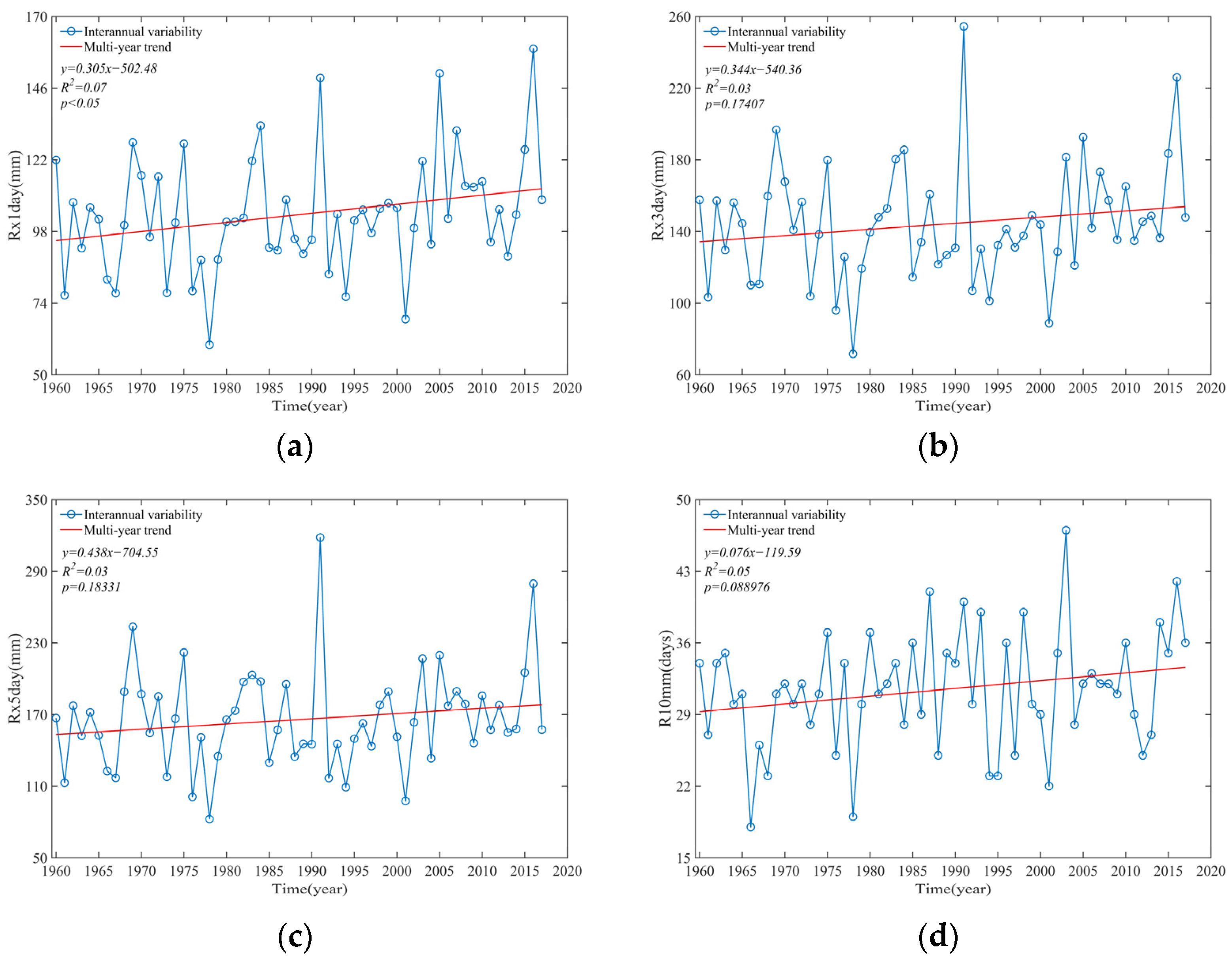
3.1. Temporal Variation in Extreme-Precipitation Indices

On the interannual scale, the Mann–Kendall test analysis showed that Rx1day, R99p, and SDII all showed a significant increasing trend in the Jianghuai region, with rates of increase of 2.7 mm·(10a)⁻¹, 2.9 mm·(10a)⁻¹, and 0.2 mm·(10a)⁻¹, respectively (

Table 3. Mann–Kendall test for monotonic trends of extreme-precipitation indices in the Jianghuai region from 1960 to 2017.

Index	Change Rate	Statistics
Rx1day	2.7 mm·(10a)−1	2.33 *
Rx3day	3 mm·(10a)−1	1.59
Rx5day	4 mm·(10a)−1	1.44
R95p	7.6 mm·(10a)−1	1.82
R99p	2.9 mm·(10a)−1	2.21 *
SDII	0.2 mm·(d⋅10a)−1	2.98 *
PRCPTOT	20.1 mm·(10a)−1	1.56
R10 mm	0.7 d·(10a)−1	1.81
R20 mm	0.2 d·(10a)−1	0.85
R50 mm	0.1 d·(10a)−1	1.70
CDD	−0.1 d·(10a)−1	0.70
CWD	0.1 d (10a)−1	−1.12

Note. * Passing a 95% confidence level.

, Figure 2a,g,k). Rx3day, Rx5day, R95p, PRCPTOT, R10 mm, R20 mm, R50 mm, and CWD showed a nonsignificant increasing trend with increasing rates of 3 mm·(10a)⁻¹, 4 mm∙(10a)⁻¹, 7.6 mm∙(10a)⁻¹, 20.1 mm·(10a)⁻¹, 0.7 d·(10a)⁻¹, 0.2 d∙(10a)⁻¹, 0.1 d∙(10a)⁻¹, and 0.1 d∙(10a)⁻¹, respectively (Table 3, Figure 2b–f,i,j,l). CDD showed a nonsignificant decreasing trend with a decrease rate of −0.1 d∙10 a⁻¹ (Table 3, Figure 2h).

The 1960–2017 period can be divided into six subperiods: 1960–1969 (T1), 1970–1979 (T2), 1980–1989 (T3), 1990–1999 (T4), 2000–2009 (T5) and 2010–2017 (T6). The interdecadal variation in extreme-precipitation indices in the Jianghuai region is shown in Figure 3. On the decadal scale, except for the CDD, all the other indices showed an upward trend, which is similar to the trend on the interannual scale, above. Rx1day, Rx3day, and Rx5day showed decreasing (T1–T2), increasing (T2–T3), decreasing (T3–T4), and increasing (T4–T6) trends. R10 mm, R20 mm, R50 mm, PRCPTOT showed increasing (T1–T3), decreasing (T3–T5), and increasing (T5–T6) trends. SDII and CWD showed increasing (T1–T4), increasing (T4–T5), and decreasing (T5–T6) trends. CDD showed decreasing (T1–T3), increasing (T3–T4), decreasing (T4–T5), and increasing (T5–T6) trends. R95p showed increasing (T1–T3), decreasing (T3–T4), and increasing (T4–T6). R99p showed decreasing (T1–T2) and increasing (T2–T6) trends. It can be seen that the trends in extreme-precipitation intensity and frequency are similar, with Rx1day, Rx3day, and Rx5day experiencing the most fluctuations. Conversely, the CWD trend is the flattest.

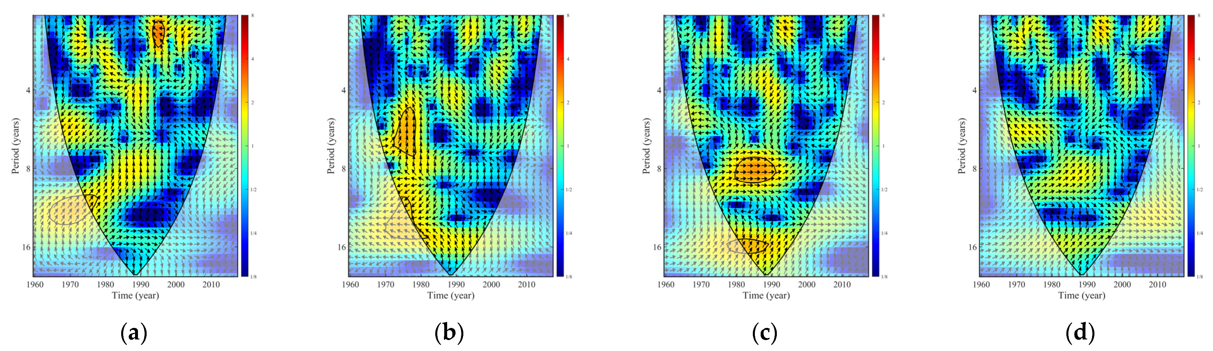
3.2. Periodic Variations in Extreme-Precipitation Indices

The CWT analysis showed that extreme-precipitation indices in the Jianghuai region contained several cycles of variation at different scales between 1960 and 2017, forming oscillation centers with positive and negative intervals at various scales, with obvious chronological and interannual variation characteristics. At the global scale, a significant cycle of variability of 5.8 years was found for R10 mm and R20 mm, which underwent seven cycles of alternation, with oscillation centers in 1961, 1970, 1979, 1988, 1997, 2006, and 2014 (Figure 4d,e). There were no significant periodic variations in the other extreme-precipitation indicators.

At the local scale, there were differences in the cyclical variability characteristics of the different extreme-precipitation indicators. Approximately 2.0~2.6 years significant cycles existed for Rx1day, R20 mm, R95p, R99p, and PRCPTOT, occurring in 2003–2006, 1992–1997, 1990–1994, 2004–2006, 1991–1996, respectively (Figure 4a,e,j–l). Significant cycles of approximately 2.00~2.6 years and 3.4~4.4 years existed for Rx3day and R50 mm, occurring in 1985–1993 and 1989–1994, respectively (Figure 4b,f). Rx5day had 2.10~2.6 years, 3.4~4.6 years, 5.4~6.1 years, and 7.3~8.0 years significant cycles, which occurred in 1990–1993, 1987–1993, 1968–1973, and 1985–1991, respectively (Figure 4c). R10 mm had 2.10~2.7 years, 3.4~4.2 years, and 4.8~6.3 years significant cycles, which occurred in 1993–1997, 2001–2004, and 1994–2004, respectively (Figure 4d). The SDII had significant cycles of 2.2~2.6 years in 1974–1977 and 1990–1996 and 3.8~4.4 years in 1988–1992 (Figure 4g). The CDD had significant cycles of 2.10~3.0 years in 1973–1980 and 11.0~16.8 years in 1975–1987 (Figure 4h). The CWD had a significant cycle of 4.8~5.6 years from 1992–1997 (Figure 4i). We found that most of the exponential periodic oscillations exist on a time scale of 2~4 years and are concentrated in the 1990s.

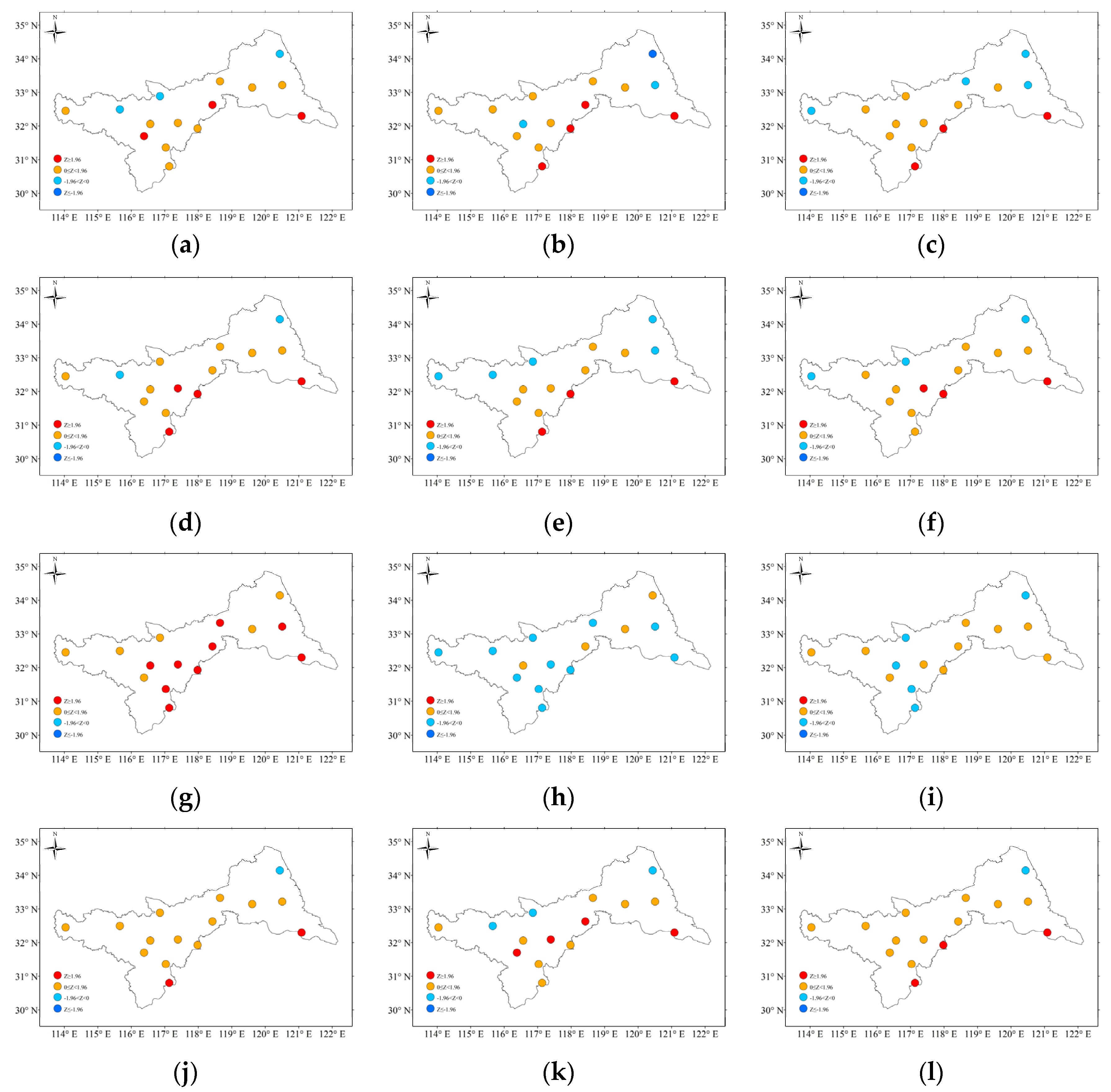
3.3. Spatial Distribution of Extreme-Precipitation Indices

To further demonstrate the spatial distribution characteristics of the change trends of different extreme-precipitation indicators, the results of the M-K trend tests of different extreme-precipitation indicators at different stations were spatially visualized. For Rx1day, Rx5day, R20 mm, R50 mm, and PRCPTOT, three stations showed a significant increasing trend and were located in the southwestern, central, and southeastern parts of the Jianghuai region; the other stations showed nonsignificant change trends (Figure 5a,c,e,f,l). For Rx3day, R10 mm and R99p, four sites showed a significant increasing trend, concentrated in the southwestern, central and southeastern parts of the Jianghuai region; among them, one site in the northeastern part of the Jianghuai region showed a significant decreasing trend for Rx3day; the other sites showed nonsignificant change trends (Figure 5b,d). For R95p, two sites showed a significant increasing trend, located in the southwestern and southeastern parts of the Jianghuai region; other sites showed nonsignificant trends (Figure 5j). For the SDII, nine sites showed a significant increasing trend, mainly in the southwestern, central and southeastern parts of the Jianghuai region; other sites showed insignificant trends (Figure 5g). For CDD and CWD, there were no sites with significant changes (Figure 5h,i).

3.4. Impacts of Atmospheric Circulation on Extreme-Precipitation Indices

3.4.1. Principal Component Analysis of Extreme-Precipitation Indices

There are certain correlations between different extreme-precipitation indices, which increase the complexity of analyses. Before exploring the influence of atmospheric circulation on extreme precipitation, principal component analysis was used to reduce the dimensionality and eliminate the correlation effect between different indices.

The principal component analysis found that the variance contributions of the first four principal components in the extreme-precipitation index were 72.71%, 10.19%, 8.03%, and 4.60%, and their cumulative contribution of variance was 95.53%, so these four principal components could characterize all 12 extreme-precipitation indices. In addition, the highest loading of R95p was 0.33 in the first principal component; the maximum loading of CDD was 0.50 and 0.82 in the second and third principal components, respectively; and the highest value of CWD loading was 0.81 in the fourth principal component (

Table 4. Principal component analysis of extreme-precipitation indices in the Jianghuai region, 1960–2017.

Component	Rx1day	Rx3day	Rx5day	R10 mm	R20 mm	R50 mm	Variance Contribution Rate (%)
1	0.31	0.31	0.31	0.28	0.30	0.31	72.71
2	0.25	0.29	0.25	−0.43	−0.28	0.15	10.18
3	−0.21	−0.13	−0.08	0.16	0.19	0.04	8.03
4	0.18	0.15	0.14	−0.20	−0.24	−0.23	4.60
component	SDII	CDD	CWD	R95p	R99p	PRCPTOT	Variance Contribution Rate (%)
1	0.30	−0.07	0.20	0.33	0.30	0.32	72.71
2	0.04	0.50	−0.37	−0.01	0.26	−0.20	10.18
3	0.20	0.82	0.33	−0.08	−0.18	0.06	8.03
4	−0.24	−0.03	0.81	−0.05	0.15	−0.18	4.60

). Therefore, R95p can represent principal component one, CDD can represent principal components two and three, and CWD can represent principal component four. By calculating the correlation coefficients among the extreme-precipitation indices, it was found that CDD was negatively correlated with the other indices and did not pass the 0.05 confidence level test; the correlation coefficients between R95p and the remaining indices were basically above 0.8, and the correlation coefficients between CWD and the other indices were 0.4–0.7 (

Table 5. Analysis of the correlation coefficients of extreme-precipitation indices in the Jianghuai region, 1960–2017.

	Rx1day	Rx3day	Rx5day	R10 mm	R20 mm	R50 mm	SDII	CDD	CWD	R95p	R99p	PRCPTOT
Rx1day	1.00	—	—	—	—	—	—	—	—	—	—	—
Rx3day	0.94	1.00	—	—	—	—	—	—	—	—	—	—
Rx5day	0.91	0.97	1.00	—	—	—	—	—	—	—	—	—
R10 mm	0.58	0.57	0.60	1.00	—	—	—	—	—	—	—	—
R20 mm	0.67	0.68	0.71	0.94	1.00	—	—	—	—	—	—	—
R50 mm	0.80	0.86	0.88	0.67	0.79	1.00	—	—	—	—	—	—
SDII	0.77	0.78	0.79	0.77	0.84	0.85	1.00	—	—	—	—	—
CDD	−0.18 *	−0.11 *	−0.10 *	−0.28 *	−0.18 *	−0.06 *	−0.02 *	1.00	—	—	—	—
CWD	0.43	0.43	0.47	0.63	0.61	0.41	0.49	−0.10 *	1.00	—	—	—
R95p	0.89	0.89	0.90	0.80	0.86	0.92	0.83	−0.26 *	0.53	1.00	—	—
R99p	0.99	0.94	0.91	0.58	0.67	0.82	0.77	−0.15 *	0.42	0.88	1.00	—
PRCPTOT	0.77	0.78	0.81	0.93	0.96	0.87	0.86	−0.25 *	0.60	0.95	0.77	1.00

Note. * Not passing the 95% confidence level.

). Therefore, R95p and CWD were used in this study to characterize the intensity and duration of extreme-precipitation events, respectively, and to analyze the influence relationship between the extreme-precipitation indices and atmospheric circulation.

3.4.2. Impacts of Atmospheric Circulation on the Duration of Extreme Precipitation

Cross wavelet transform analysis showed that CWD had a significant resonant period of 2~4 years with AO, NAO, ONI and SOI during 1965–1974, in which CWD was positively correlated with AO and SOI and negatively correlated with NAO and ONI; AO, NAO, and ONI were ahead of CWD, while SOI lagged behind CWD (Figure 6c–e,g). There were significant resonance cycles of 3~4 years with EASM, ONI, and SOI during 1993–1997, in which EASM and ONI were negatively correlated with CWD and both lagged behind CWD; SOI was positively correlated with CWD and was ahead of CWD (Figure 6a,e,f). In addition, there were significant resonance cycles of 4~6 years between CWD and ONI, PDO, SOI, and WP during 1990–2000, in which ONI, PDO, and WP were positively correlated with CWD and lagged behind CWD; SOI was negatively correlated with CWD and was ahead CWD (Figure 6e–h). Within the high band of 15~16 years, only CWD and AO had a significant resonance cycle in 1981–1991, and AO lagged behind CWD and did not show a positive or negative correlation (Figure 6c).

Cross wavelet coherence analysis showed significantly high and negative correlations between the CWD and the NAO and WP during 1964–1974 in cycles of 2 to 4 years, with NAO lagging behind CWD and WP ahead of CWD (Figure 7d,h). Significantly high correlations of 5~7 years were found between EASM and NAO from 1967 to 1975, both with negative correlations, with EASM ahead of CWD and NAO lagging behind CWD (Figure 7a,d). There was a significantly high correlation of 8~13 years with the EASM during 1973–1998, and the EASM lagged behind CWD, and a partial positive correlation between the two (Figure 7a); there was a significantly high correlation of 13~18 years with SCSMI, AO, and NAO during 1979–1994; SCSMI, AO, and NAO lagged behind CWD, SCSMI and CWD were negatively correlated, and AO and NAO showed a positive correlation with CWD (Figure 7b–d). In addition, CWD had significantly high correlations with PDO and WP from 1988 to 2001 in the 4~6-year band, all of which were positive, and WP lagged behind CWD (Figure 7f,h); the same significantly high correlation region was found with ONI and SOI, and the relative phases of the two regions were opposite (Figure 7e,g).

In general, in terms of the duration of extreme precipitation, we found that there is a certain resonance period between CWD and atmospheric circulation index. However, there are obvious differences in different time domains. These findings confirm the complex nonlinear relationships between the extreme precipitation and atmospheric circulation index. According to the significant resonance period, NAO and EASM have the most significant effect on CWD. We also found that the duration of extreme precipitation decreases in subsequent years when strong EASM occurs on the 4~8-year time scale, while the opposite is true on the 8~16-year time scale.

3.4.3. Impacts of Atmospheric Circulation on the Intensity of Extreme Precipitation

The cross wavelet transform analysis showed that there were significant resonance cycles of 2~3 years between R95p and EASM and WP during 1993–1997, 1988–1993, and 2001–2005, which were negatively correlated, and EASM and WP lagged behind R95p (Figure 8a,h); there were significant resonance cycles of 3~4 years with ONI and SOI during 1984–1990, with ONI ahead of R95p and being positively correlated, and SOI lagging behind R95p and being negatively correlated (Figure 8e,g). During 1989–1994, 1973–1979, and 1993–1999, there were significant resonance cycles of 4~6 years with PDO, SOI, and WP, respectively; PDO and WP lagged behind R95p and did not show positive or negative correlations; SOI was ahead of R95p and showed positive correlations (Figure 8f,g,h). In addition, there were 5~7-year significant resonance cycles between R95p and SCSMI in 1972–1979, with SCSMI lagging behind R95p and partially showing a positive correlation (Figure 8b); there were 7~9-year significant resonance cycles with AO in 1980–1991, showing a positive correlation (Figure 8c); there were 8~11-year significant resonance cycles with WP in 1975–1986, and WP was ahead of R95p with a negative correlation (Figure 8h).

Cross wavelet coherence analysis showed that R95p had 2~3-year significantly high correlations with AO and WP during 1973–1976 and 2001–2008, respectively, with AO and WP lagging behind R95p; AO was not positively or negatively correlated with R95p, and WP showed a negative correlation with R95p (Figure 9c,h). R95p had 3~5-year significantly high correlations with SCSMI, AO, and NAO during 1991–2002, 1982–1993, and 1982–1990 and SCSMI, AO, and NAO were ahead of R95p; among the indices, the SCSMI showed positive correlations with R95p, and AO and NAO showed negative correlations with R95p (Figure 9b–d). During 1967–1974, 1966–1975, 2006–2011, 2005–2011, and 1969–1983, there were 5~6-year significant high correlations with EASM, NAO, ONI, PDO, and SOI; among them, EASM and NAO were positively correlated with R95p, and the remaining three were negatively correlated with R95p; NAO lagged behind R95p, and the remaining four indices were ahead of R95p (Figure 9a,d–g). In addition, there were 8~9-year significant high and positive correlations between R95p and AO in 1980–1992, 15~20-year significant high correlations in 1981–1995, and AO lagged behind R95p (Figure 9c).

In terms of extreme-precipitation intensity, these observations also confirm the complex nonlinear relationships between R95p and atmospheric circulation index. AO and EASM had the most significant effect on R95p. The effect of EASM on the intensity of extreme precipitation is the same as its duration effect.

4. Discussion

The response of the hydrological cycle to climate change can be reflected by changes in precipitation. Understanding the variation in precipitation is key to the scheduling and management of water resources and water conservancy projects. The Jianghuai region is an area with a high incidence of extreme-precipitation events in China, and these events are very likely to lead to flooding, causing serious socioeconomic losses and risks to public safety. Therefore, studying the changes in precipitation in this region can provide a scientific basis for solving agricultural and environmental problems. Li et al. [60] and Guan et al. [61] studied extreme-precipitation indices in the middle and lower reaches of the Yangtze River and found that indices such as Rx1day, R99p, and SDII showed a significant increasing trend. Similar to previous studies, this study found that all extreme-precipitation indices showed an increasing trend, except for CDD, which showed a nonsignificant decreasing trend. The Rx1day, R99p, and SDII all showed a significant increasing trend, indicating that the extreme-precipitation frequency in the region did not change significantly and the precipitation intensity increased significantly; the latter was the main factor causing the change in precipitation in the region, which was similar to the findings of previous research [27,62,63], while also indicating a gradual increase in the contribution of intense precipitation [64]. Managers in the region need to focus on strengthening short-term drainage work and improving drainage standards to prevent floods, urban waterlogging, and farmland waterlogging. At the interdecadal scale, the highest mean extreme-precipitation indices were reached in 2010–2017, which indicates that extreme-precipitation events occurred frequently in recent years. Numerous survey results also showed that as the climate warms, extreme-precipitation events will occur more frequently in the future, which should be given warranted attention [28,29,30,31,32].

Extreme precipitation is one of the main causes of natural disasters, such as droughts, floods, and their alternations, with critical impacts on agricultural production and sustainable development. As a whole, the variations in extreme-precipitation indices in the southern part of the Jianghuai region, except for CWD and CDD, showed an increasing trend, while the northern part showed a decreasing trend, indicating that there were more extreme-precipitation events in the southern part of the region than in the northern part [65]. In the technical specifications of Chinese farmland drainage engineering, Rx1day and Rx3day are important indices that play important roles in the design and implementation of farmland drainage engineering. This study found that some sites in the southwestern, central, and southeastern regions of the Jianghuai region showed a significant increasing trend, while CDD and CWD showed a nonsignificant trend, indicating an increased risk of flooding to agricultural production in these regions. Miao et al. [66] similarly concluded that the increase in heavy precipitation events in the Jianghuai region may cause flooding and urban waterlogging problems.

Atmospheric circulation is an important environmental factor contributing to the variation in regional precipitation, and it is crucial to the spatial and temporal distribution and inter- and intra-annual variability in precipitation [63,67]. Most previous studies on the influence of atmospheric circulation on extreme precipitation have used the correlation coefficient method, which reflects the degree of influence of atmospheric circulation on extreme precipitation and the main influence index by calculating the correlation coefficient [11]. However, different atmospheric circulation indices and different time periods have different effects on extreme-precipitation indicators [68]. We found that AO and EASM have the most significant effects in terms of extreme-precipitation intensity (R95p), while NAO and EASM have the most significant effects in terms of extreme-precipitation duration (CWD); therefore, EASM is the atmospheric circulation index with the most significant effect on extreme-precipitation events in this study area according to cross wavelet transform and wavelet coherence analyses [69]. Further analysis in this study found that extreme precipitation in the region decreases in subsequent years when a strong EASM occurs within a 4~8-year time scale [70]; SOI and ONI have significant positive correlations with CWD and R95p in the high- and low-energy region spectra, indicating that El Niño—Southern Oscillation (ENSO) has an impact on the persistent growth in precipitation events and the increase in precipitation intensity in the region, which is consistent with the findings of Yu and Zhai [42]. Influenced by the atmospheric circulation index, the extreme-precipitation indices in the Jianghuai region show different periodic variability at different time scales. Wavelet analysis shows that, at the global scale, a significant variation cycle of 5.8 years exists for R10 mm and R20 mm, and no significant variation cycle exists for other extreme-precipitation indicators. In addition, the effect between the atmospheric circulation index and extreme precipitation is not significant in some years, suggesting that the extreme-precipitation regime is influenced not only by atmospheric oscillation but also by topography [71] and human activities [21].

5. Conclusions

In this study, 12 extreme-precipitation indices were calculated based on the measured daily precipitation records from 15 meteorological stations in the Jianghuai region from 1960 to 2017. During this study period, the spatiotemporal evolution patterns of extreme precipitation in the Jianghuai region and their correlations with eight atmospheric circulation indices were analyzed by the Mann–Kendall test, wavelet analysis, cross wavelet transform and wavelet coherence methods, and the following conclusions were drawn:

• Rx1day, R99p, and SDII in the Jianghuai region showed a significant increasing trend; Rx3day, Rx5day, R95p, PRCPTOT, R10 mm, R20 mm, R50 mm, and CWD showed a nonsignificant increasing trend; and CDD showed a nonsignificant decreasing trend. The intensity of extreme precipitation has increased significantly, and extreme-precipitation events of shorter durations and higher intensities have become more frequent.
• The periodic oscillations of most indices tend toward 2~4-year scales and are concentrated in the 1990s. At the global scale, there was a significant change cycle of 5.8 years for R10 mm and R20 mm.
• Sites with significant increases in Rx1day, Rx3day, Rx5day, R10 mm, R20 mm, R50 mm, SDII, R95p, R99p and PRCPTOT were located in the southwestern, central and southeastern parts of the Jianghuai region; sites with significant decreases in Rx3day were located in the northeastern part of the Jianghuai region; and there were sites with no significant changes in CDD and CWD. An intensified precipitation system will increase the risk of flooding and urban inundation in the Jianghuai region, especially concentrated in the southern part of the region, where the intensity and frequency of extreme precipitation may increase more rapidly.
• Both the extreme-precipitation indices and the atmospheric circulation index had significant resonance periods, but there were obvious differences in time domains. EASM is the most significant influence of atmospheric-circulation index on extreme-precipitation events in the Jianghuai region in this study.

References

1. Song, F.; Qi, H.; Wei, H.; Ho, C.H.; Li, R.; Tang, Z. Projected climate regime shift under future global warming from multi-model, multi-scenario CMIP5 simulations. Glob. Planet. Change 2014, 112, 41–52. [Google Scholar]
2. IPCC. Climate Change: The Physical Science Basis. Contribution of Working Group I to the Sixth Assessment Report of the Intergovernmental Panel on Climate Change; Cambridge University Press: Cambridge, UK, 2021. [Google Scholar]
3. Trenberth, K.E. Atmospheric Moisture Residence Times and Cycling: Implications for Rainfall Rates and Climate Change. Clim. Change 1998, 39, 667–694. [Google Scholar] [CrossRef]
4. Trenberth, K.E.; Dai, A.; Rasmussen, R.M.; Parsons, D.B. The changing character of precipitation. B Am. Meteorol Soc. 2003, 84, 1205–1217. [Google Scholar] [CrossRef]
5. Sena, J.A.; de Deus, L.A.B.; Freitas, M.A.V.; Costa, L. Extreme Events of Droughts and Floods in Amazonia: 2005 and 2009. Water Resour. Manag. 2012, 26, 1665–1676. [Google Scholar] [CrossRef]
6. Papalexiou, S.M.; Montanari, A. Global and Regional Increase of Precipitation Extremes under Global Warming. Water Resour. Res. 2019, 55, 4901–4914. [Google Scholar] [CrossRef]
7. Houze, R.A.; Rasmussen, K.L.; Medina, S.; Brodzik, S.R.; Romatschke, U. Anomalous Atmospheric Events Leading to the Summer 2010 Floods in Pakistan. Bull. Am. Meteorol. Soc. 2011, 92, 291–298. [Google Scholar] [CrossRef]
8. Khaing, Z.M.; Zhang, K.; Sawano, H.; Shrestha, B.B.; Sayama, T.; Nakamura, K. Flood hazard mapping and assessment in data-scarce Nyaungdon area, Myanmar. PLoS ONE 2019, 14, e0224558. [Google Scholar]
9. Zhang, K.; Liu, L.; Chao, L.; Yang, J. Spatiotemporal variations of terrestrial ecosystem water use efficiency in Yunnan Province from 2000 to 2014. Water Resour. Prot. 2019, 35, 1–5. [Google Scholar]
10. Rosenzweig, C.; Tubiello, F.N.; Goldberg, R.; Mills, E.; Bloomfield, J. Increased crop damage in the US from excess precipitation under climate change. Glob. Environ. Change-Hum. Policy Dimens. 2002, 12, 197–202. [Google Scholar] [CrossRef] [Green Version]
11. Liu, S.Y.; Huang, S.Z.; Xie, Y.Y.; Leng, G.Y.; Huang, Q.; Wang, L.; Xue, Q. Spatial-temporal changes of rainfall erosivity in the loess plateau, China: Changing patterns, causes and implications. Catena 2018, 166, 279–289. [Google Scholar] [CrossRef]
12. Alexander, L.V.; Zhang, X.; Peterson, T.C.; Caesar, J.; Gleason, B.; Tank, A.M.G.K.; Haylock, M.; Collins, D.; Trewin, B.; Rahimzadeh, F.; et al. Global observed changes in daily climate extremes of temperature and precipitation. J. Geophys. Res. -Atmos. 2006, 111, 1042–1063. [Google Scholar] [CrossRef] [Green Version]
13. Madsen, H.; Lawrence, D.; Lang, M.; Martinkova, M.; Kjeldsen, T.R. Review of trend analysis and climate change projections of extreme precipitation and floods in Europe. J. Hydrol. 2014, 519, 3634–3650. [Google Scholar] [CrossRef] [Green Version]
14. Hu, K.; Huang, G.; Huang, P.; Kosaka, Y.; Xie, S.-P. Intensification of El Niño-induced atmospheric anomalies under greenhouse warming. Nat. Geosci. 2021, 14, 377–382. [Google Scholar] [CrossRef]
15. Martinkova, M.; Kysely, J. Overview of Observed Clausius-Clapeyron Scaling of Extreme Precipitation in Midlatitudes. Atmosphere 2020, 11, 786. [Google Scholar] [CrossRef]
16. Obubu, J.P.; Mengistou, S.; Fetahi, T.; Alamirew, T.; Odong, R.; Ekwacu, S. Recent Climate Change in the Lake Kyoga Basin, Uganda: An Analysis Using Short-Term and Long-Term Data with Standardized Precipitation and Anomaly Indexes. Climate 2021, 9, 179. [Google Scholar] [CrossRef]
17. Mo, C.; Ruan, Y.; He, J.; Jin, J.L.; Liu, P.; Sun, G. Frequency analysis of precipitation extremes under climate change. Int. J. Climatol. 2018, 39, 1373–1387. [Google Scholar] [CrossRef]
18. Donat, M.G.; Lowry, A.L.; Alexander, L.V.; O’Gorman, P.A.; Maher, N. More extreme precipitation in the world’s dry and wet regions. Nat. Clim. Change 2016, 6, 508–513. [Google Scholar] [CrossRef]
19. Gu, G.J.; Adler, R.F.; Huffman, G.J.; Curtis, S. Tropical rainfall variability on interannual-to-interdecadal and longer time scales derived from the GPCP monthly product. J. Clim. 2007, 20, 4033–4046. [Google Scholar] [CrossRef]
20. Yang, Y.; Gan, T.Y.; Tan, X. Spatiotemporal changes in precipitation extremes over Canada and their teleconnections to large-scale climate patterns. J. Hydrometeorol. 2018, 20, 275–296. [Google Scholar] [CrossRef]
21. Wiel, K.V.D.; Kapnick, S.B.; Oldenborgh, G.J.V.; Whan, K.; Cullen, H. Rapid attribution of the August 2016 flood-inducing extreme precipitation in south Louisiana to climate change. Hydrol. Earth Syst. Sci. 2017, 21, 897–921. [Google Scholar] [CrossRef] [Green Version]
22. Zhao, Y.F.; Zou, X.Q.; Cao, L.G.; Xu, X.W.H. Changes in precipitation extremes over the Pearl River Basin, southern China, during 1960–2012. Quat. Int. 2014, 333, 26–39. [Google Scholar] [CrossRef]
23. Zhang, M.; Chen, Y.N.; Shen, Y.J.; Li, B.F. Tracking climate change in Central Asia through temperature and precipitation extremes. J. Geogr. Sci. 2019, 29, 3–28. [Google Scholar] [CrossRef] [Green Version]
24. Fujibe, F.; Yamazaki, N.; Katsuyama, M.; Kobayashi, K. The Increasing Trend of Intense Precipitation in Japan Based on Four-Hourly Data for a Hundred Years. Sola 2005, 1, 41–44. [Google Scholar] [CrossRef] [Green Version]
25. Gao, T.; Xie, L.A. Study on progress of the trends and physical causes of extreme precipitation in China during the last 50 years. Adv. Earth Sci. 2014, 29, 577–589. [Google Scholar]
26. Yue, D.; Jiang, W.; He, B.; Zheng, C.; Kai, J. Change in Intensity and Frequency of Extreme Precipitation and Its Possible Teleconnection with Large-Scale Climate Index over the China from 1960 to 2015. J. Geophys. Res. Atmos. 2018, 123, 2068–2081. [Google Scholar]
27. Zhai, P.M.; Zhang, X.B.; Wan, H.; Pan, X.H. Trends in total precipitation and frequency of daily precipitation extremes over China. J. Clim. 2005, 18, 1096–1108. [Google Scholar] [CrossRef]
28. Huang, X.; Stevenson, S.; Hall, A.D. Future Warming and Intensification of Precipitation Extremes: A "Double Whammy" Leading to Increasing Flood Risk in California. Geophys. Res. Lett. 2020, 47, e2020GL088679. [Google Scholar] [CrossRef]
29. Tariku, T.B.; Gan, T.Y. Regional climate change impact on extreme precipitation and temperature of the Nile river basin. Clim. Dyn. 2018, 51, 3487–3506. [Google Scholar] [CrossRef]
30. Colmet-Daage, A.; Sanchez-Gomez, E.; Ricci, S.; Llovel, C.; Servat, E. Evaluation of uncertainties in mean and extreme precipitation under climate change for northwestern Mediterranean watersheds from high-resolution Med and Euro-CORDEX ensembles. Hydrol. Earth Syst. Sci. Discuss. 2018, 22, 673–687. [Google Scholar] [CrossRef] [Green Version]
31. Forestieri, A.; Arnone, E.; Blenkinsop, S.; Candela, A.; Fowler, H.; Noto, L.V. The impact of climate change on extreme precipitation in Sicily, Italy. Hydrol. Processes 2018, 32, 332–348. [Google Scholar] [CrossRef] [Green Version]
32. Aihaiti, A.; Jiang, Z.; Zhu, L.; Li, W.; You, Q. Risk changes of compound temperature and precipitation extremes in China under 1.5 °C and 2 °C global warming. Atmos. Res. 2021, 264, 105838. [Google Scholar] [CrossRef]
33. Hatzaki, M.; Wu, R.G. The south-eastern Europe winter precipitation variability in relation to the North Atlantic SST. Atmos. Res. 2015, 152, 61–68. [Google Scholar] [CrossRef]
34. Kotsias, G.; Lolis, C.J.; Hatzianastassiou, N.; Levizzani, V.; Bartzokas, A. On the connection between large-scale atmospheric circulation and winter GPCP precipitation over the Mediterranean region for the period 1980–2017. Atmos. Res. 2015, 152, 61–68. [Google Scholar] [CrossRef]
35. Mao, R.; Gong, D.Y.; Yang, J.; Bao, J.D. Linkage between the Arctic Oscillation and winter extreme precipitation over central-southern China. Clim. Res. 2011, 50, 187–201. [Google Scholar] [CrossRef] [Green Version]
36. Gu, X.; Zhang, Q.; Chen, X.; Fan, K. The spatiotemporal rates of heavy precipitation occurrence at difference scales in China. J. Hydraul. Eng. 2017, 48, 505–515. [Google Scholar]
37. Payne, A.E.; Demory, M.E.; Leung, L.R.; Ramos, A.M.; Shields, C.A.; Rutz, J.J.; Siler, N.; Villarini, G.; Hall, A.; Ralph, F.M. Responses and impacts of atmospheric rivers to climate change. Nat. Rev. Earth Environ. 2020, 1, 143–157. [Google Scholar] [CrossRef] [Green Version]
38. Waliser, D.; Guan, B. Extreme winds and precipitation during landfall of atmospheric rivers. Nat. Geosci. 2017, 10, 179–183. [Google Scholar] [CrossRef]
39. Whan, K.; Sillmann, J.; Schaller, N.; Haarsma, R. Future changes in atmospheric rivers and extreme precipitation in Norway. Clim. Dyn. 2020, 54, 2071–2084. [Google Scholar] [CrossRef] [Green Version]
40. Wang, T.; Wei, K.; Jiao, M.A. Atmospheric Rivers and Mei-yu Rainfall in China:A Case Study of Summer 2020. Adv. Atmos. Sci 2021, 38, 2137–2152. [Google Scholar] [CrossRef]
41. Sun, Z.B.; Chen, X.F.; Zhang, Q.; Song, C.Q.; Song, W.D.; Huang, X.M. Spatiotemporal patterns of extreme percipitation regimes in the Wanjiang region from 1960 to 2014. J. Beijing Norm. Univ. Nat. Sci. Ed. 2018, 54, 11. [Google Scholar]
42. Yu, R.; Zhai, P.M. The influence of EI Nino on summer persistent preciptation structure in the middle and lower reaches of the Yangtze River and its possible mechanism. Acta Meteorol. Sin. 2018, 76, 408–419. [Google Scholar]
43. Cannon, A.J. Revisiting the nonlinear relationship between ENSO and winter extreme station precipitation in North America. Int. J. Clim. 2015, 35, 4001–4014. [Google Scholar] [CrossRef]
44. Liu, F.; Zhang, H.Q. Land Use Structure and Temporal-Spatial Variation Analysis in Eight Main Agricultural Regions in China. Resour. Sci. 2011, 33, 294–301. [Google Scholar]
45. Qian, Y.F.; Wang, Q.Q.; Huang, D.Q. Studies of Floods and Droughts in the Yangtze-Huaihe River Basin. Chin. J. Atmos. Sci. 2007, 31, 1279–1289. [Google Scholar]
46. Wu, J.L.; Zhu, H.F.; Zong, P.S.; Hui, P.H.; Tang, J.P. Analysis on the spatial-temporal features of temperature extremes in the Yangtze-Huaihe river basin over the past decades: Comparison between observation and reanalysis. J. Meteorol. Sci. 2018, 38, 13. [Google Scholar]
47. Kousari, M.R.; Zarch, M.A.A.; Ahani, H.; Hakimelahi, H. A survey of temporal and spatial reference crop evapotranspiration trends in Iran from 1960 to 2005. Clim. Change 2013, 120, 277–298. [Google Scholar] [CrossRef]
48. Li, Z.X.; He, Y.Q.; Wang, P.Y.; Theakstone, W.H.; An, W.L.; Wang, X.F.; Lu, A.G.; Zhang, W.; Cao, W.H. Changes of daily climate extremes in southwestern China during 1961–2008. Glob. Planet. Change 2012, 80, 255–272. [Google Scholar]
49. Song, X.Y.; Song, S.B.; Sun, W.Y.; Mu, X.M.; Wang, S.Y.; Li, J.Y.; Li, Y. Recent changes in extreme precipitation and drought over the Songhua River Basin, China, during 1960–2013. Atmos. Res. 2015, 157, 137–152. [Google Scholar] [CrossRef]
50. Tong, S.Q.; Li, X.Q.; Zhang, J.Q.; Bao, Y.H.; Bao, Y.B.; Na, L.; Si, A.L. Spatial and temporal variability in extreme temperature and precipitation events in Inner Mongolia (China) during 1960–2017. Sci. Total Environ. 2019, 649, 75–89. [Google Scholar] [CrossRef]
51. Fu, G.; Chen, S.; Liu, C.; Shepard, D. Hydro-Climatic Trends of the Yellow River Basin for the Last 50 Years. Clim. Change 2004, 65, 149–178. [Google Scholar] [CrossRef] [Green Version]
52. Chaouche, K.; Neppel, L.; Dieulin, C.; Pujol, N.; Ladouche, B.; Martin, E.; Salas, D.; Caballero, Y. Analyses of precipitation, temperature and evapotranspiration in a French Mediterranean region in the context of climate change. Comptes Rendus Géoscience 2010, 342, 234–243. [Google Scholar] [CrossRef]
53. Huo, Z.L.; Dai, X.Q.; Feng, S.Y.; Kang, S.Z.; Huang, G.H. Effect of climate change on reference evapotranspiration and aridity index in arid region of China. J. Hydrol. 2013, 492, 24–34. [Google Scholar] [CrossRef]
54. Thiel, H. A rank-invariant method of linear and polynomial regression analysis, Part 3. Neth. Akad. Van Wettenschappen Proc. 1950, 59, 1397–1412. [Google Scholar]
55. Sen, P.K. Estimates of the Regression Coefficient Based on Kendall’s Tau. Publ. Am. Stat. Assoc. 1968, 63, 1379–1389. [Google Scholar] [CrossRef]
56. Ling, H.B.; Xu, H.L.; Fu, J.Y. Temporal and Spatial Variation in Regional Climate and Its Impact on Runoff in Xinjiang, China. Water Resour. Manag. 2013, 27, 381–399. [Google Scholar] [CrossRef]
57. Jolliffe, I.T. Principal Component Analysis; Springer: Berlin/Heidelberg, Germany, 1986. [Google Scholar]
58. Torrence, C.; Compo, G.P. A Practical Guide to Wavelet Analysis. Bull. Am. Meteorol. Soc. 1998, 79, 61–78. [Google Scholar] [CrossRef] [Green Version]
59. Wu, S.Q.; Zhao, W.J.; Yang, Y.; Jin, N.N.; Zheng, D.Y.; Wang, X.Y. Response of extreme precipitation events in the middle and lower reaches of the Yangtze River Basin to the atmospheric circulation based on continuous wavelet transform. J. Water Resour. Water Eng. 2021, 32, 67–76. [Google Scholar]
60. Li, X.; Zhang, K.; Gu, P.R.; Feng, H.T.; Yin, Y.F.; Chen, W.; Cheng, B.C. Changes in precipitation extremes in the Yangtze River Basin during 1960–2019 and the association with global warming, ENSO, and local effects. Sci. Total Environ. 2021, 760, 144244. [Google Scholar] [CrossRef]
61. Guan, Y.; Zheng, F.; Zhang, X.; Wang, B. Trends and variability of daily precipitation and extremes during 1960–2012 in the Yangtze River Basin, China. Int. J. Climatol. 2016, 37, 1282–1298. [Google Scholar] [CrossRef]
62. Zhang, Q.; Peng, J.T.; Xu, C.Y.; Singh, V.P. Spatiotemporal variations of precipitation regimes across Yangtze River Basin, China. Theor. Appl. Climatol. 2014, 115, 703–712. [Google Scholar] [CrossRef]
63. Zhang, Q.; Xu, C.Y.; Zhang, Z.X.; Chen, Y.Q.D.; Liu, C.L.; Lin, H. Spatial and temporal variability of precipitation maxima during 1960–2005 in the Yangtze River basin and possible association with large-scale circulation. J. Hydrol. 2008, 353, 215–227. [Google Scholar] [CrossRef]
64. Fang, S.D.; Jiang, Z.H. Analysis of the Change in the Precipitation Intensity Distribution in the Yangze–Huaihe River Basin under Global Warming. Clim. Environ. Res. 2013, 18, 757–766. [Google Scholar]
65. Wang, J.; Yu, J.H.; He, J.Q. Study on characteristics and change trend of extreme rainfall in the Jianghuai region. Clim. Environ. Res. 2015, 20, 80–88. [Google Scholar]
66. Miao, C.; Duan, Q.; Sun, Q.; Lei, X.; Li, H. Non-uniform changes in different categories of precipitation intensity across China and the associated large-scale circulations. Environ. Res. Lett. 2018, 14, 025004. [Google Scholar] [CrossRef]
67. Wang, Y.Q.; Zhou, L. Observed trends in extreme precipitation events in China during 1961–2001 and the associated changes in large-scale circulation (vol 32, art no L09707, 2005). Geophys. Res. Lett. 2005, 32. [Google Scholar] [CrossRef]
68. Nalley, D.; Adamowski, J.; Biswas, A.; Gharabaghi, B.; Hu, W. A multiscale and multivariate analysis of precipitation and streamflow variability in relation to ENSO, NAO and PDO. J. Hydrol. 2019, 574, 288–307. [Google Scholar] [CrossRef]
69. Zhang, J.; Zhi, X.F.; Miao, K. Characteristics of the quasi-biennial oscillation of the summer precipitation over Yangtze-Huaihe Valley and its correlation factors. Trans. Atmos. Sci. 2014, 37, 541–547. [Google Scholar]
70. Yin, Y.X.; Chen, H.S.; Zhai, P.M.; Xu, C.Y.; Ma, H.D. Characteristics of summer extreme precipitation in the Huai River basin and their relationship with East Asia summer monsoon during 1960–2014. Int. J. Climatol. 2019, 39, 1555–1570. [Google Scholar] [CrossRef]
71. Wang, L.; Chen, S.; Zhu, W.; Ren, H.; Zhu, L. Spatiotemporal variations of extreme precipitation and its potential driving factors in China’s North-South Transition Zone during 1960–2017. Atmos. Res. 2021, 252, 105429. [Google Scholar] [CrossRef]
Figure 1. Locations of the Jianghuai Region and selected meteorological stations.
Sustainability 14 06680 g001
Figure 2. Interannual variation in extreme-precipitation indices in the Jianghuai region from 1960 to 2017. (a) Rx1day, (b) Rx3day, (c) Rx5day, (d) R10 mm, (e) R20 mm, (f) R50 mm, (g) SDII, (h) CDD, (i) CWD, (j) R95p, (k) R99p, (l) PRCPTOT.
Sustainability 14 06680 g002aSustainability 14 06680 g002b
Figure 3. Interdecadal variation in extreme-precipitation indices in the Jianghuai region, 1960–2017. (a) Rx1day, (b) Rx3day, (c) Rx5day, (d) R10 mm, (e) R20 mm, (f) R50 mm, (g) SDII, (h) CDD, (i) CWD, (j) R95p, (k) R99p, (l) PRCPTOT. The red dots represent the average for the decade. The red plus sign indicates the discrete points for that decade.
Sustainability 14 06680 g003aSustainability 14 06680 g003b
Figure 4. Wavelet analyses of extreme-precipitation indices during the study period. (a) Rx1day, (b) Rx3day, (c) Rx5day, (d) R10 mm, (e) R20 mm, (f) R50 mm, (g) SDII, (h) CDD, (i) CWD, (j) R95p, (k) R99p, (l) PRCPTOT. The black solid line represents the wavelet influence cone, the black contoured dashed line depicts the 5% significance level relative to the red noise, and the significance level red solid line is the red noise test with a 95% confidence level. The more the color is biased toward dark red, the higher power and higher cycle intensity.
Sustainability 14 06680 g004aSustainability 14 06680 g004b
Figure 5. Changes in the spatial distribution of extreme-precipitation indices, 1960–2017. (a) Rx1day, (b) Rx3day, (c) Rx5day, (d) R10 mm, (e) R20 mm, (f) R50 mm, (g) SDII, (h) CDD, (i) CWD, (j) R95p, (k) R99p, (l) PRCPTOT.
Sustainability 14 06680 g005
Figure 6. Cross wavelet energy spectrum between CWD and atmospheric-circulation indices. (a) CWD-EASM, (b) CWD-SCSMI, (c) CWD-AO, (d) CWD-NAO, (e) CWD-ONI, (f) CWD-PDO, (g) CWD-SOI, (h) CWD-WP. Thick black contour lines delineate the 5% significance level for red noise. COI, pictures that may distort the edges, are represented in lighter tones. Right (left) pointing arrows show an in-phase (anti-phase) relationship, and vertically downward arrows show that the Atmospheric Circulation Index leads CWD by 90° (one-quarter). Red (blue) represents stronger (weaker) power.
Sustainability 14 06680 g006
Figure 7. Wavelet coherence spectrum between CWD and atmospheric circulation indices. (a) CWD-EASM, (b) CWD-SCSMI, (c) CWD-AO, (d) CWD-NAO, (e) CWD-ONI, (f) CWD-PDO, (g) CWD-SOI, (h) CWD-WP. Thick black contour lines delineate the 5% significance level for red noise. COI, pictures that may distort the edges, are represented in lighter tones. Right (left) pointing arrows show an in-phase (anti-phase) relationship, and vertically downward arrows show that the Atmospheric Circulation Index leads CWD by 90° (one-quarter). Red (blue) represents stronger (weaker) power.
Sustainability 14 06680 g007
Figure 8. Cross wavelet energy spectrum between R95p and atmospheric circulation indices. (a) R95p-EASM, (b) R95p-SCSMI, (c) R95p-AO, (d) R95p-NAO, (e) R95p-ONI, (f) R95p-PDO, (g) R95p-SOI, (h) R95p-WP. Thick black contour lines delineate the 5% significance level for red noise. COI, pictures that may distort the edges, are represented in lighter tones. Right (left) pointing arrows show an in-phase (anti-phase) relationship, and vertically downward arrows show that the Atmospheric Circulation Index leads R95p by 90° (one-quarter). Red (blue) represents stronger (weaker) power.
Sustainability 14 06680 g008aSustainability 14 06680 g008b
Figure 9. Wavelet coherence spectrum between R95p and atmospheric Ccirculation indices. (a) R95p-EASM, (b) R95p-SCSMI, (c) R95p-AO, (d) R95p-NAO, (e) R95p-ONI, (f) R95p-PDO, (g) R95p-SOI, (h) R95p-WP. Thick black contour lines delineate the 5% significance level for red noise. COI, pictures that may distort the edges, are represented in lighter tones. Right (left) pointing arrows show an in-phase (anti-phase) relationship, and vertically downward arrows show that the Atmospheric Circulation Index leads R95p by 90° (one-quarter). Red (blue) represents stronger (weaker) power.
Sustainability 14 06680 g009