Abstract
Dynamic customer demands impose new challenges for vehicle routing optimization with time windows, in which customer demands appear dynamically within the working periods of depots. The delivery routes should be adjusted for the new customer demands as soon as possible when new customer demands emerge. This study investigates a collaborative multidepot vehicle routing problem with dynamic customer demands and time windows (CMVRPDCDTW) by considering resource sharing and dynamic customer demands. Resource sharing of multidepot across multiple service periods can maximize logistics resource utilization and improve the operating efficiency of delivery logistics networks. A bi-objective optimization model is constructed to optimize the vehicle routes while minimizing the total operating cost and number of vehicles. A hybrid algorithm composed of the improved k-medoids clustering algorithm and improved multiobjective particle swarm optimization based on the dynamic insertion strategy (IMOPSO-DIS) algorithm is designed to find near-optimal solutions for the proposed problem. The improved k-medoids clustering algorithm assigns customers to depots in terms of specific distances to obtain the clustering units, whereas the IMOPSO-DIS algorithm optimizes vehicle routes for each clustering unit by updating the external archive. The elite learning strategy and dynamic insertion strategy are applied to maintain the diversity of the swarm and enhance the search ability in the dynamic environment. The experiment results with 26 instances show that the performance of IMOPSO-DIS is superior to the performance of multiobjective particle swarm optimization, nondominated sorting genetic algorithm-II, and multiobjective evolutionary algorithm. A case study in Chongqing City, China is implemented, and the related results are analyzed. This study provides efficient optimization strategies to solve CMVRPDCDTW. The results reveal a 32.5% reduction in total operating costs and savings of 29 delivery vehicles after optimization. It can also improve the intelligence level of the distribution logistics network, promote the sustainable development of urban logistics and transportation systems, and has meaningful implications for enterprises and government to provide theoretical and decision supports in economic and social development.
1. Introduction
The vehicle routing problem (VRP) is a combinatorial optimization problem with multiple practical applications in transportation, distribution, and collection [1,2,3]. In a classic VRP, a fleet of vehicles from depots serves a geographically spread group of customers with known demands and then returns to the depots. The optimization goal is to find an ideal distribution solution with minimum distances or other objectives while satisfying the customer demands, routing constraints, vehicle restrictions, and depot limitations. The widespread applications of VRP in the logistics field have resulted in the intense development of its variants in the literature, for instance, multidepot VRP (MDVRP) [4,5,6]), VRP with time windows (VRPTW) [7,8], MDVRPTW [9,10], and multiperiod VPR [11,12].
Most researchers define all customers’ demands as known with certainty in advance. They also investigate various optimization problems in stationary environments. Nevertheless, new customer orders may emerge over time and need to be integrated into the preplanned delivery schemes in most real-world applications [13]. Therefore, the VRP with dynamic customer demands and time windows (VRPDCDTW) extends the VRPTW by considering the dynamic customer demands (DCDs). The VRPDCDTW is a partial dynamic VRPTW, where some demands are known when the delivery routes are planned. In comparison, the other demands emerge dynamically during the work period of depots. Customers should be served within their required specific time windows; otherwise, additional penalties are imposed for time window violations (late and early arrival of vehicles) [14,15]. The DCDs originate from the uncertainty in the arrival time of customer orders, which requires the decision makers to update delivery schemes based on the latest information (customer demands, time windows, and vehicle remaining capacity) [13]. A dynamic insertion strategy (DIS) is designed as a vehicle routing updating method to coordinate static customer demands (SCDs) and DCDs and tackle the dynamic optimization problem.
Moreover, most studies focus on VRPDCDTW for a single depot [16,17,18]. The multidepot VRPDCDTW (MVRPDCDTW) can incorporate the practical consideration of large-scale distribution networks to promote collaboration and resource sharing among multiple depots. The development of communication and information technologies in recent years has resulted in the recognition of collaboration as an important strategy to improve the effectiveness of the urban transportation systems and reduce the total operating cost (TOC) of the delivery process [19,20]. In competitive markets, the supplier, manufacturer, and retailer are willing to collaborate and share costs, which facilitates a sustainable supply chain [21,22]. In this study, resource sharing is adopted to achieve customer service sharing (CSS) and transportation resource sharing (TRS) among multiple service periods to optimize collaborative MVRPDCDTW (CMVRPDCDTW). The improved k-medoids clustering algorithm implements the CSS by reassigning customers to depots based on the nearest distance. Furthermore, an improved multiobjective particle swarm based on the DIS (IMOPSO-DIS) algorithm optimizes delivery routes in terms of the TOC and number of vehicles (NV).
Three types of the problem considering dynamic customer demands have been widely investigated in recent years, including VRPTW with stochastic customer demands, VRPTW with SCDs and DCDs, and VRPTW with dynamic and stochastic customer demands [2,23,24]. Most papers study the VRPTW with DCDs in a single depot logistics network. In this study, a collaborative MDVRP with SCDs and DCDs is studied in a multidepot logistics network. The optimized routes with SCDs are generated in advance, and then DCDs can be inserted into the existing optimization routes with consideration of the time windows of other customers in the route and the remaining capacity of vehicles. When dealing with the multidepot optimization problem, a hybrid intelligent algorithm including the clustering algorithm and heuristic algorithm can achieve a good performance [12,15]. The clustering algorithm can be used to simplify the network complexity, and then the multiobjective heuristic algorithms are often utilized to obtain Pareto optimal solutions [25,26]. A hybrid algorithm including the improved k-medoids clustering algorithm and IMOPSO-DIS algorithm can instantly obtain the insertion position information of DCDs and the vehicle sharing routes among multiple depots. In addition, the effective combination and design of multidepot collaboration and DIS strategies with IMOPSO algorithm are also further discussed. Therefore, the proposed model and algorithm in this study can effectively ensure the timeliness of DCD service while ensuring that enterprises reduce logistics operating costs.
The rest of this study is arranged as follows. Section 2 lists the related works of CMVRPDCDTW. Section 3 provides a problem statement and a multiobjective optimization model. Section 4 describes a solution methodology consisting of customer clustering and heuristic algorithms. Section 5 conducts a case study in Chongqing City, China to validate the effectiveness of the proposed model and approach. Section 6 summarizes the optimization results of this study and mentions future works.
2. Literature Review
This section briefly reviews VRPDCDTW, MVRPDCDTW, and CMVRPDCDTW first. Several computational intelligence methods, including genetic algorithm (GA) [27], ant colony optimization (ACO) [28], variable neighborhood search (VNS) [17], and particle swarm optimization (PSO) [29], have been modified to seek the optimal vehicle routes with DCDs. Finally, we elaborate on the limitations of the related literature and the contributions of this work.
2.1. VRPDCDTW
In VRPDCDTW optimization, customers are visited within their required service time windows, and the DCDs that appear during the working periods of the depot are also studied [30,31,32]. In recent years, different dynamic factors such as uncertain service times [33], new customer demands [17,34], demand prediction [35,36,37], and road traffic congestion [38] have been investigated in various real-life applications. Peled et al. [39] studied the impact of demand prediction accuracy on the dynamic public transportation performance. Kuo et al. [13] formulated a dynamic VRPTW (DVRPTW) model considering uncertain service times. They solved this model by applying an improved fuzzy ant colony system to maximize the number of customers and minimize the waiting time (WT). Chen et al. [40] studied a DVRPTW with the limited NV and decomposed DVRP into a series of static VRPs to tackle new customer demands. Laganà et al. [41] proposed a dynamic multiperiod general routing problem arising in postal service and parcel delivery companies and planned the vehicle routes with dynamically fluctuating demands. Xue et al. [42] proposed a two-echelon DVRP with proactive satellite stations, and DCDs were served by the delivery vehicles from a specific transfer station in the second-echelon network.
2.2. MVRPDCDTW
The continuous expansion of the delivery logistics network scale has resulted in an increasing number of researchers who study MDVRP to optimize the multidepot logistics networks [43,44,45]. Bae and Moon [9] expanded MDVRPTW to a delivery and installation study of electronics and considered the goal of minimizing the fixed cost (FC) of depots and vehicles, travel distances, and labor expenses. Zhen et al. [46] investigated MDVRPTW by considering the release date of customers’ packages. A hybrid of PSO and GA algorithms was designed to solve this problem with the minimum total traveling time. Fan et al. [10] optimized vehicle routing using a hybrid GA in a multidepot distribution network and considered travel time, time windows, FC of vehicles, and fuel consumption. Sadati et al. [47] presented a variable tabu neighborhood search algorithm for addressing a class of MDVRP including MDVRPTW and multidepot open VRP. Although many scholars have studied MDVRPTW from multiple perspectives, few studies have combined DCDs with MDVRPTW. Therefore, the present work integrates the two to propose MVRPDCDTW, which has some theoretical significance.
2.3. CMVRPDCDTW
In recent years, the concepts of collaboration and sharing have been introduced in many studies to realize the efficient configuration of resources, thereby promoting cost and resource savings through multidepot collaboration [48,49,50]. Many third-party platforms are created to provide sharing services, which promote various collaboration modes [51,52]. Wei et al. [53] investigated a matching problem for ride-sourcing markets. Effective information sharing and online matching make ride-sourcing services more efficient and timely. Muñoz-Villamizar et al. [54] studied a collaborative transport network in which companies are encouraged to share customer service to reduce transportation costs (TCs), the NV, and the negative impact on the environment of delivery activities. Vaziri et al. [55] proposed a VRP with fair carrier collaboration. The vehicle capacities and transportation requests were shared in an alliance formed by multiple carriers to eliminate empty backhauls, enhance vehicle utilization and improve the profit of participants. Zhang et al. [56] investigated a heterogeneous multidepot collaborative VRP. Joint route planning, product transfer of multidepot, and impact of depot locations and allocation of benefits on outcomes of collaboration were explored. The above studies have illustrated the advantages of different collaboration modes including sharing customers, vehicle capacity, and forming collaborative alliances. In the present study, we design a collaborative mode in which customer services and transportation resources can be shared among multiple depots in different service periods.
2.4. Related Solution Methodologies
The majority of the existing studies employ intelligent optimization algorithms to find near-optimal solutions for the VRP because of the limitations of exact algorithms in solving large-scale VRPs and their variants [57,58,59]. The solution methodologies in related literature have great reference value for the present study. Table 1 lists the main objectives considered and solution methods used to optimize various VRP variants that have been proposed in the literature.

Table 1.
A summary of the related literature.
Khouadjia et al. [67] studied a VRP with dynamic requests and the dynamic adapted PSO algorithm and VNS were designed to optimize this problem. The information obtained previously on the search space was used to respond to DCDs. AbdAllah et al. [68] developed an enhanced GA that attempts to increase diversity and the ability to discard local optima and find a high-quality solution for DVRP. Xiang et al. [23] proposed a demand coverage diversity adaptation method in the ACO algorithm to respond effectively to the newly appeared customer demands by maintaining the diversity of covered customers. Many scholars focus on multiobjective optimization models as the research progresses [64,69]. Therefore, multiobjective optimization algorithms, such as multiobjecitve PSO (MOPSO) [70], nondominated sorting GA-ΙΙ (NSGA-ΙΙ) [71], and multiobjective evolutionary algorithm (MOEA) [72] are developed to find Pareto optimal solutions for multiobjective optimization problems (MOOPs).
Wang et al. [66] formulated a multiobjective optimizing model by minimizing the total route distance and total customer WT to solve DVRPTW. An improved MOEA was designed to make relative optimal routing schemes by enhancing the diversity and accelerating the convergence. Niu et al. [73] considered three objectives including travel distance, driver remuneration, and the NV, to optimize the VRP with stochastic demands. Moreover, a machine learning algorithm was exploited to find Pareto front of solutions. Zarouk et al. [74] suggested a routing and scheduling problem that considers stochastic demands, varying travel times, driving time, and soft service time windows. A hybrid heuristic method consisting of GA and simulated annealing was devised to minimize energy consumption and maximize customer satisfaction. Therefore, a bi-objective CMVRPDCDTW optimization model with minimum TOC and NV is formulated in this study to cope with environmental changes and ensure service quality.
However, the previous research has several limitations, which can be summarized as follows: (1) Most studies focusing on VRPDCDTW and CMVRPDCDTW have not been adequately investigated. (2) The collaboration mode among multiple depots is seldom considered, particularly in a logistics network with DCDs. (3) Many optimization models consider only a single objective when the objective functions, such as total distance, WT, NV, and TOC, are formulated. (4) The existing heuristic approaches and evolutionary algorithms are inefficient in solving CMVRPDCDTW.
Compared with the previous research on optimizing vehicle routing, the present study provides the following contributions: (1) A delivery logistics network with DCDs and time windows is developed to study the proposed CMVRPDCDTW. (2) CSS and TRS are designed to facilitate collaboration among multiple depots for sustainable development of the logistics network. (3) A bi-objective optimization model is established to minimize the TOC and NV, including time windows, multiple service periods, delivery, and transportation constraints. (4) An IMOPSO-DIS is proposed to coordinate SCDs and DCDs and the performance of the proposed approach is validated by a real-world case study.
3. Problem Statement and Model Formulation
3.1. Problem Statement
The goal of CMVRPDCDTW is to design an efficient distribution logistics network that can dynamically plan the route for delivery vehicles through resource sharing among depots. The distribution logistics network has two types of customer demands: (i) SCDs, which are known before planning routes, and (ii) DCDs, which appear dynamically within the working periods of depots. In addition, customers with service time windows are served by delivery vehicles during a certain period, and each vehicle departs from and returns to the same depot within the depot’s time window. The comparison of the CMVRPDCDTW before and after optimization is shown in Figure 1.
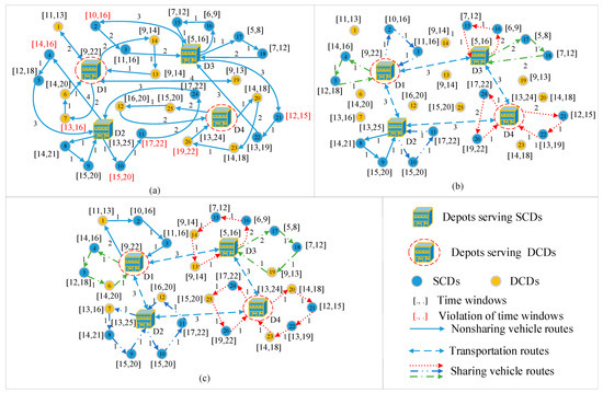
Figure 1.
Illustration of the CMVRPDCDTW optimization. (a) Nonoptimized logistics network with dynamic customer demands; (b) Preoptimized logistics network with dynamic customer demands; (c) Optimized logistics network with dynamic customer demands
In Figure 1a, four depots (i.e., D1, D2, D3, and D4) and 26 customer demand nodes are distributed in the logistics network, where DCDs are served by vehicles from D1 and D4 and SCDs are served by vehicles from D2 and D3. Each depot only serves its customer yielding long-distance and cross-haul transportation. For instance, customers 24 and 21 are closer to D4 but are served by D2 and D3, respectively. In addition, vehicles must be temporarily arranged (e.g., D1→C19→D1 and D1→C1→D1) to serve DCDs because of the dynamic nature of DCD emergence time and its time window constraints; thus, the capacity of vehicles is not fully utilized. Moreover, the violation of time windows is inevitable without a reasonable vehicle scheduling scheme. Therefore, an effective optimization strategy should be implanted to increase the utilization rate of transportation resources and improve the operational efficiency of the distribution network.
The delayed processing strategy is proposed to deal with DCDs by deferring DCDs to the next time interval and treating them as SCDs. First, the routes of SCDs are preoptimized as shown in Figure 1b. Then, DIS is applied to meet SCDs and DCDs simultaneously by dynamically adjusting delivery routes as shown in Figure 1c. In Figure 1b,c, the customer services and transportation resources are shared among four depots to redesign the distribution logistics network. The customers are assigned to the nearest depots by sharing customer services, thereby contributing to the reduction in violation of time windows and the elimination of unreasonable vehicle routes. Given the change in customers in depots after CSS, the goods are transferred among depots through centralized transportation by semitrailer trucks. The vehicle can also be shared among the same or different depots. For instance, routes D3→C16→C15→C14→C13→D3, D4→C20→C21→C22→C23→D4, and D4→C24→C25→C26→D4 are visited by a vehicle in different service periods. Therefore, compared with the nonoptimized network, the optimized logistics network has considerable advantages in terms of operating cost and efficiency.
For calculation purposes, the following assumptions are made: the TC is $40 per time unit, the distribution cost (DC) is $30 per time unit, the penalty cost (PC) is $20 per time unit, the insertion cost (IC) per additional time unit incurred to visit the DCDs is $20, and the maintenance cost (MC) of each semitrailer truck and delivery vehicle is $200 and $100, respectively. All the costs, number of semitrailer trucks (NST), and NV before and after CMVRPDCDTW optimization are listed in Table 2.
Table 2.
Comparison before and after CMVRPDCDTW optimization.
In Table 2, the TOC is decreased from $3720 to $2350, whereas the NV is reduced by 9. In addition, the distribution cost is decreased by 48.6%, the PC is decreased by $260, and the TC and IC are increased to $480 and $160, respectively, after optimization. The cost reductions far outweigh the cost increases. Consequently, resource sharing and DIS play major roles in reducing TOCs and transportation resources in a collaborative multidepot logistics network with DCDs.
3.2. Definitions
The notation definitions of sets, parameters, and decision variables related to the CMVRPDCDTW optimization model are listed in Table 3. Moreover, several reasonable assumptions of the optimization model are listed as follows:
Table 3.
Definitions and notations.
Assumption 1.
Each delivery vehicle starts and ends its route at the same depot.
Assumption 2.
The number of DCDs steadily fluctuates within one service period.
Assumption 3.
SCDs have the characteristics of periodic service and depots need to first generate optimized routes with SCDs, while DCDs need to be inserted into the existing optimized routes considering the time windows of customers in the routes and residual loading capacity of vehicles.
3.3. Model Formulation
In this section, CMVRPDCDTW is formulated as a bi-objective mathematical programming model considering centralized transportation among depots and distribution between depots and customers. This model aims to determine an optimal vehicle routing scheme by minimizing the TOC and NV. The objective functions are shown as follows.
F1 is composed of the TOC of semitrailer trucks Z1, TOC of delivery vehicles Z2, PC Z3, IC, and FC Z4 to minimize the TOC in the logistics network. F2 represents minimizing the NV through vehicle sharing.
Z1 includes two components in Equation (3): represents total TC and expresses MC of semitrailer trucks.
Z2 in Equation (4) is composed of the total DC and MC of delivery vehicles.
Z3 in Equation (5) is the PC of semitrailer trucks and delivery vehicles for earliness and delay. is the PC of trucks for earliness and is the PC of trucks for delay. is the PC of vehicles for earliness and is the PC of vehicles for delay.
Z4 in Equation (6) denotes the FC of depots and the IC of DCD. is the FC of depots. is the IC of DCD that depends on additional travel distances generated by visiting the inserted DCDs in an existing route.
Subject to:
Constraints (7) and (8) indicate that trucks and vehicles have enough capacity to satisfy the total demands of assigned depots and customers. Constraint (9) denotes that total customer demands cannot exceed the capacity of the corresponding depot. Constraints (10) and (11) represent each depot and customer only served by one truck or vehicle within a service period. Constraints (12) and (13) ensure flow conservation of trucks and vehicles, respectively. Constraint (14) expresses that DCDs must occur within the depot’s time windows. Constraints (15) and (16) ensure that each truck’s departure and arrival time do not violate the time windows of depots. Constraints (17) and (18) guarantee that each vehicle departs and returns to the depot within the depot’s time window. Constraints (19)–(22) define the departure time and arrival time of vehicles. Constraints (23) and (24) are used to eliminate the subtour of semitrailer trucks and delivery vehicles, respectively. Constraints (25)–(29) specify the binary decision variable used in this model.
4. Solution Methodology
The proposed CMVRPDCDTW model in this study model belongs to NP-hard and MOOPs. The concepts of Pareto and nondominated are integrated into the metaheuristic algorithms to solve large-scale MOOPs within a reasonable computational time [75]. Among the well-known multiobjective metaheuristic algorithms, MOPSO has been utilized extensively by many researchers owing to its excellent performance in finding approximate Pareto solutions [26,70,76]. Therefore, a hybrid algorithm combining the improved k-medoids clustering algorithm and IMOPSO-DIS is proposed as the solution methodology.
The improved k-medoids clustering algorithm groups customers with similar characteristics (e.g., geographical locations and time windows) into the same clustering units. CSS is achieved by customer clustering operation. Then, the IMOPSO-DIS is conducted for delivery route optimization by minimizing TOC and NV. In the IMOPSO-DIS algorithm, the external archive updating strategy and elitist learning strategy (ELS) are utilized to maintain the diversity of the swarm and avoid particles trapped in local optimal. Then, the DIS is adopted to update solutions with the farthest insertion heuristic. The flowchart of the solution methodology is presented in Figure 2.
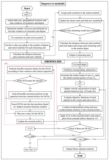
Figure 2.
Flowchart of solution methodology for CMVRPDCDTW optimization.
4.1. Customer Clustering
Customer clustering is an effective way to simplify the collaborative multidepot logistics network. The k-medoids clustering algorithm is a widely utilized clustering algorithm, and it clusters customers into k clusters based on the distance between customers and medoids [25,77]. The k-medoids clustering algorithm is less sensitive to the outlier data and the use of dissimilarity between nodes makes k-medoids more robust than other clustering algorithms [78]. In addition, the k-medoids clustering algorithm can effectively combine with many heuristic methods to assign customers into different groups by minimizing the distances between customers [79]. The improved k-medoids clustering algorithm is adopted in this study to assign each customer to k clusters W = {w1, w2, …, wk} according to the temporal–spatial distance between medoids and customers. The temporal–spatial distance D (i, j) between medoid i and customer j can be computed by Equations (30) and (31).
where (xi, yi), (xj, yj), and (tj, tj) indicate the latitudes, longitudes, and middle point of time windows of medoid i and customer j, respectively. In addition, α, β, and γ are the corresponding coefficients. The objective function of the improved k-medoids clustering algorithm is to minimize the total cost TCih when customer h replaces medoid i, as shown in Equation (32).
The improved k-medoids algorithm processing is divided into three steps. First, k customers are randomly selected as medoids of initial k clusters, and the remaining customers are assigned to the nearest clusters according to the distance from medoids. Second, medoids are repeatedly replaced with nonmedoids to improve the clustering quality until the clustering results no longer change. Finally, the distance from each medoid to each depot is calculated, and each clustering unit is assigned to the closest depot. Algorithm 1 shows the procedure of the improved k-medoids clustering algorithm.
| Algorithm 1: Improved k-medoids clustering |
| Input: Set of customers and depots, the number of clustering units k |
| Output: k clustering units Steps: (1) Randomly select k customers as medoids (2) Repeat (i) Calculate the distance between medoids and customers (ii) Assign the customers to the nearest clusters (iii) Randomly select customer h to replace medoid i (iv) Calculate the total cost TCih when new clusters are formed (v) If TCih > 0 then Replace medoid i with the customer h and update the set of medoids End (3) Until clustering results no longer change (4) Calculate the distance between each medoid and each depot (5) Assign each clustering unit to the nearest depot (6) Output k clustering units |
4.2. IMOPSO-DIS
The MOPSO algorithm is regarded as an efficient algorithm, successfully utilized in various MOOPs [70,80,81]. PSO algorithm was first presented by Eberhart and Kennedy [82]. Coello et al. [83] developed the MOPSO to deal with the MOOPs by integrating the Pareto dominance and utilizing the external archive to store nondominated solutions. The complexity of this model requires an effective algorithm that is well equipped to solve MOOPs. IMOPSO-DIS is designed to address CMVRPDCDTW. The pseudocode of the used IMOPSO-DIS algorithm is shown in Algorithm 2.
| Algorithm 2: IMOPSO-DIS |
| Input: Clustering units (coordinates, time windows, and demands), i_max (number of maximum iteration), Npop (size of the swarm), Narc (capacity of the external archive), c1 (personal learning coefficient), c2 (global learning coefficient), w (inertia weight), γ (elitist learning rate) |
| Output: Nondominated particles in the external archive Steps: (1) Initialize the particles in the swarm P0 (vp,0, xp,0) (2) Evaluate each particle in P0 and Nondominated sorting (P0) (3) Initialize the external archive A0 by nondominated solution maintaining (4) Initialize pbestp,0 and gbest0 (5) While i< i_max do (6) For each particle p = 1: Npop (7) Update the velocity and position by using Equations (33) and (34) (8) Evaluate the new particle (9) Update pbestp,i (10) End for (11) Ai←External archive updating (Ai−1) (12) Select gbesti according to the crowding distance (13) If rand () < γ (14) Update Ai by ELS (15) End If (16) While DCD d appears do (17) For each particle p in Ai (18) xp,i←DIS (d, xp,i) and update Ai (19) End for (20) End while (21) i = i + 1 (22) End while (23) Output results in the external archive |
4.2.1. Particle Updating
In the MOPSO algorithm, each particle defined by its current position and velocity represents a potential solution. The particles search the solution space based on their personal best (pbest) and global best (gbest) of the entire swarm. The velocity vp,i and position xp,i of particle p at iteration i are updated by Equations (33) and (34).
where pbestp,i and gbesti are the best position of particle p and the best position of the entire swarm at ith iteration, respectively. c1 and c2 are constants used to specify the particle acceleration toward xpbest,i and xgbest,i. r1 and r2 are random numbers between 0 and 1. The w is the inertial weight and adjusts the trade-off between the global and local search abilities. The decreasing linear inertia weight is calculated as follows:
where i and i_max represent the current iteration and maximum iteration of the algorithm, respectively. wmin and wmax are the lower and upper bounds of inertia weight.
In the MOPSO algorithm, determining the leadership during the search process, retaining the nondominated solution to obtain the optimal Pareto front, and maintaining the diversity of particle swarm to jump out a local optimal are important issues to be addressed. Therefore, the IMOPSO-DIS proposed in this study finds Pareto optimal solutions for CMVRPDCDTW.
4.2.2. Selection of pbest and Nondominated Sorting
The selection of leaders is a key procedure in IMOPSO-DIS optimization because the search is largely influenced by the pbset and gbset. In a single objective optimization problem, the leader is the particle with the best position in the swarm. However, in multiobjective problems, the optimum solutions are a set of nondominated solutions from the Pareto front. For a two-objective minimization problem, u = [u1, u2] and v = [v1, v2] are assumed to be two particles; thus, u1, u2, v1, and v2 are the objective values in function f(x) = [f1(x), f2(x)]. If u1 < v1 and u2 < v2, then u dominates v and vice versa. If there are no other particles in the swarm that dominate u, the particle u is a nondominated solution.
The selection pbset can be summarized as follows. If xpbest,i dominates xpbest,i−1, then xpbest,i−1 is replaced by xpbest,i and vice versa. If no dominance relationship exists between them, then the pbset is chosen randomly from them. The gbset is selected from nondominated solutions obtained by nondominated sorting. Figure 3 illustrates nondominated sorting processing for a two-objective minimization problem.
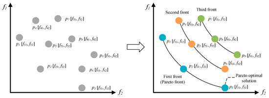
Figure 3.
Nondominated sorting processing.
In Figure 3, the jth particle uses two vectors [fj1, fj2] to classify the swarm and guide the search toward Pareto optimal solutions. The Pareto optimal solutions represented in blue circles (p1, p2, p3) are nondominated by any other solutions in the entire swarm, and a Pareto front is composed of Pareto optimal solutions. The solutions in the second front (p4, p5, p6) are the feasible solutions dominated by Pareto optimal solutions in the first front. Similarly, the green circles are solutions (p7, p8, p9) dominated by solutions in the second front. The detailed steps of nondominated sorting are presented in Algorithm 3.
| Algorithm 3: Nondominated sorting |
| Input: Particle swarm P = {p1, p2, p3, …, pj}, rank counter r |
| Output: r and a set of particles in different ranks Steps: (1) Initialize rank counter r as 0 (2) Repeat (i) r←r + 1 (ii) Evaluate the particles (iii) Find the nondominated particles from P based on the dominance relationship (iv) Assign rank r to these particles (v) Remove these particles from P (3) Until the P←ø (4) Output the nondominated soring results |
4.2.3. External Archive Updating Strategy and Gbest Selection
An external archive is widely utilized to retain nondominated particles obtained by the MOPSO algorithm [84,85]. The selection of gbset is determining a nondominated particle from the archive as xgbest,i. IMOPSO-DIS uses crowding distance for archive updating and xgbest,i selection by calculating the relative density of nondominated particles in the external archive [86]. The crowding distance of particle j is defined as Equation (36).
where and are the mth objective function of particle j + 1 and j − 1, and and represent maximum and minimum values of mth objective function, respectively. The external archive updating algorithm is shown in Algorithm 4.
| Algorithm 4: External archive updating |
| Input: External archive Ai−1, new particle swarm P = {p1, p2, p3, …, pj}, Narc |
| Output: Updated external archive Ai Steps: (1) Ai←Ai−1 (2) For j= 1: |j| (3) Evaluate the new particle pj (4) If new particle pj is dominated by any particles in Ai (5) New particle pj cannot add to Ai (6) Else (7) Ai←Ai ∪ pj (8) End if (9) End for (10) If |Ai|> Narc (11) Nondominated sorting (Ai) (12) For j = 1: |Ai| (13) Calculate the CD(j) by Equation (38) (14) End for (15) Remove the particle with the lowest CD from Ai (16) End if (17) Output Ai |
In Algorithm 4, the new particles are compared with all existing particles in the external archive one by one. If the new particle is dominated by any particle in the archive, then it cannot be stored in the archive; otherwise, the new particle should be added to the archive. As an increasing number of nondominated particles are added, the archive capacity inevitably grows, thereby reducing the search efficiency and enhancing the computational cost of the algorithm. Accordingly, crowding distance is introduced to control archive capacity from exceeding the predefined value. The particles in a relatively high-density area tend to be deleted to maintain the diversity of the swarm. The nondominated particle with the highest CD value in the archive is selected as gbset, as shown in Figure 4.
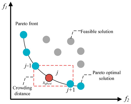
Figure 4.
The gbset selection based on crowding distance.
4.2.4. ELS
The particles need to be prevented from converging to the local optima during optimization; therefore, an ELS is applied in this study to help particles jump out of the local optima, thus improving the global search capability of the IMOPSO-DIS [87,88]. The ELS performs mutation on the gbest and guides it to a better region. The rest of the particles in the archive follows xgbest,i to the new region. Accordingly, the particles in the external archive are mutated.
The ELS randomly selects one dimension of the gbset with the same probability for each selection. The ELS is performed via Gaussian perturbation as follows:
where gbestd is the dth dimension of gbest, and and are the lower and upper bounds of the optimized problem in the dth dimension. Gaussian (μ, γ2) is a Gaussian distribution random number with a mean μ = 0 and standard deviation γ, shown as Equation (38).
where R refers to the elitist learning rate, which decreases linearly with the number of iterations; γmax = 1 and γmin = 0.1 are the upper and lower bounds of the learning scale, respectively; i is the current number of iterations, and i is the maximum number of iterations.
4.2.5. DIS
After the Pareto optimal solutions for all SCDs are found by IMPSO-DIS, a DIS is designed to insert DCDs into the most appropriate positions in the executing static routes via the farthest insertion heuristic [40,89]. DIS updates the statics routes in terms of the vehicle capacity, the times that DCDs come up, the location of DCDs, and time windows of the depots. The new vehicles should be arranged from depots for DCDs when the vehicles are overloaded or cannot arrive within the time window of depots after the insertion operation is conducted. Some checks must be performed before insertion to ensure the feasibility of the insertion.
Check 1 Vehicle capacity
First, the vehicle whose capacity meets Constraint (41) is found in executing static routes. If this vehicle has enough goods to meet the DCDs, then time windows are checked.
Check 2 Time windows
Constraint (40) indicates the time of DCD d that comes up in the rth service period. Constraint (41) ensures that vehicle v can arrive at the depot within its time window.
If one of the above checks fails, in other words, no feasible insertion position for DCDs exists, then a new vehicle satisfying Constraint (42) should be dispatched from the depot to serve DCDs; otherwise, DIS is applied to add DCDs to the particles from the external archive Ai containing all SCDs obtained by IMOPSO-DIS.
First, all feasible insertion points in particle p for each DCD d are searched. Second, the objective function value increments Δfij(d) are calculated after each DCD is inserted into a feasible insertion point. Third, the feasible insertion point with minimum Δfij(d) is selected as the best insertion point for each DCD. Fourth, the Δfij(d) of each DCD is compared and the DCD with the maximum Δfij(d) according to Equation (43) is inserted into its best insertion position.
where Δfij(d) is the objective function value increment when the DCD d is inserted between customer i and j. Finally, the xp,i and Ai are updated. The pseudocode of the DIS is shown in Algorithm 5, and an example of the dynamic insertion process is presented in Figure 5.
| Algorithm 5: DIS |
| Input: External archive Ai−1, new particle swarm P = {p1, p2, p3, …, pj}, Narc |
| Output: Updated external archive Ai Steps: (1) While DCDs exist, do (2) For each DCD d (3) Perform the feasibility insertion checks (4) If DCD d can be inserted into xp,i (5) Feasible insertion points in xp,i are found (6) Calculate Δfij(d) after inserting d (7) Choose the insertion point with minimum Δfij(d) as the best insertion point for DCD (8) Else (9) Plan a new route for DCD (10) xp,i←xp,i∪d (11) End If (12) End for (13) Compare the Δfij(d) of each DCD d (14) Insert DCD d with the maximum Δfij(d) into the best insertion point (15) Update xp,i and external archive Ai (16) End while (17) Output the external archive Ai |
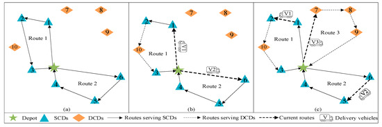
Figure 5.
Dynamic insertion process.(a) Optimal delivery routes of SCDs; (b) Insertion of DCD 10; (c) Updated delivery routes
In Figure 5a, Routes 1 and 2 are planned for six SCDs (i.e., 1, 2, 3, 4, 5, and 6) by the IMOPSO-DIS algorithm and four DCDs (i.e., 7, 8, 9, and 10) are to be served. In Figure 5b, the DIS is applied to insert DCDs to the best insertion points. The point between SCDs 2 and 3 is selected as the best insertion point for DCD 10, whereas the other DCDs (i.e., 7, 8, and 9) do not pass the feasible insertion checks. In Figure 5c, DCD 10 is added to Route 1 traveled by V1, and a new route (i.e., Route 3 traveled by V3) is planned to serve those DCDs that cannot be inserted into the existing delivery routes. Route 2, traveled by V2, is not changed in the dynamic insertion process.
5. Implementation and Analysis
5.1. Algorithm Comparison
Three prominent multiobjective optimization algorithms, NSGA-ΙΙ [90], MOPSO [91], and MOEA [92], compare with the IMOPSO-DIS algorithm. Thirteen MDVRPTW instances are gathered from the database of the NEO research group (https://neo.lcc.uma.es/vrp/vrp-instances/multiple-depot-vrp-with-time-windows-instances/, accessed on 3 February 2022) and are used to verify the superiority of the proposed algorithm in solving the CMVRPDCDTW optimization problem. The 13 MDVRPTW instances are modified and expanded to 26 CMVRPDCDTW instances by turning some customer demands into DCDs. The details of 26 instances are shown in Table 4.
Table 4.
Description of 26 CMVRPDCDTW instances.
Table 4 shows the characteristics of 26 CMVRPDCDTW instances including the number of depots, number of SCDs, number of DCDs, and capacity of vehicles. NSGA-ΙΙ, MOPSO, MOEA, and IMOPSO-DIS algorithms are adopted to find nondominated solutions for the proposed model. The related parameters of NSGA-ΙΙ and MOEA are determined as follows: population size (Npop = 100), maximum number of iterations (i_max = 100), mutation rate (r_mu = 0.1), and crossover rate (r_cr = 0.9). The MOPSO and IMOPSO-DIS factors are population size (Npop = 100), the maximum number of iterations (i_max = 100), personal acceleration coefficient (c1 = 1), global acceleration coefficient (c2 = 2), lower bound of inertia weight (wmin = 0.4), upper bound of inertia weight (wmax = 0.9), and external archive size (Narc = 50). The results of each instance including TOC, NV, and WT, calculated by NSGA-ΙΙ, MOPSO, MOEA, and IMOPSO-DIS algorithms, are presented in Table 5 and Figure 6.
Table 5.
Comparison of optimization results of IMOPSO-DIS, MOPSO, NSGA-ΙΙ, and MOEA.
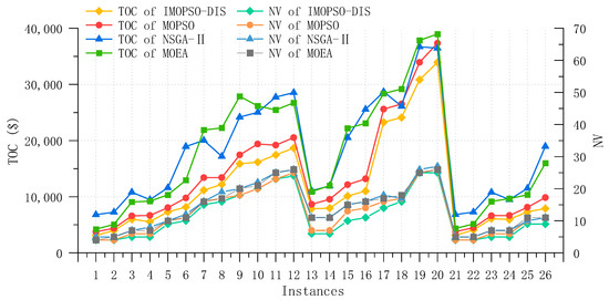
Figure 6.
Comparison of TOC and NV of the three algorithms in 26 instances.
The optimization results in Table 5 demonstrate that IMOPSO-DIS is superior to MOPSO, NSGA-ΙΙ, and MOEA in terms of minimizing the TOC, NV, and WT. The average value of the TOC calculated by IMOPSO-DIS is $11,896, which is $1532, $6171, and $5739 lower than that by MOPSO, NSGA-ΙΙ, and MOEA, respectively. Moreover, the average value of NV is minimum (12) in IMOPSO-DIS is smaller than the average values of NV in MOPSO (13), NSGA-ΙΙ (14), and MOEA (14). The average value of WT calculated by IMOPSO-DIS (93 min) is also smaller than the average values of WT calculated by the other three algorithms. As shown in Figure 6, the TOCs optimized with the IMOPSO-DIS and MOPSO algorithms are close to each other, and both are better than the calculated results of NSGA-ΙΙ and MOEA. The difference in the NV computed by the four algorithms is slight, at approximately 0–2 vehicles. Accordingly, the IMOPSO-DIS algorithm has higher reliability and robustness results in solving the CMVRPDCDTW optimization problem compared to MOPSO, NSGA-ΙΙ, and MOEA.
5.2. Case Study
5.2.1. Data Description and Parameter Setting
A real multidepot logistics network with DCDs in Chongqing, China is selected to evaluate the effectiveness and applicability of the proposed optimization model and solution methodology in solving the CMVRPDCDTW. The network consists of five depots (D1, D2, D3, D4, and D5) and 200 customers (C1, C2, …, C200), of which 70 are the number of customers with dynamic demands and 130 are the number of customers with static demands. The geographic location distribution and initial characteristics of depots and customers are shown in Figure 7 and Table 6.
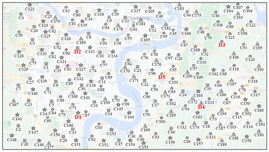
Figure 7.
Geographic location distribution of depots and customers.
Table 6.
Initial characteristics of depots and their customers.
In Table 6, D1, D3, and D5, and their customers with static demands are represented by pentagrams, diamonds, and circles, respectively. Squares and triangles refer to D2 and D4 and the customers with dynamic demands they serve. The number of customers served by the five depots is 44, 36,43,34, and 43.
5.2.2. Customer Clustering Results
The implementation of the collaboration mode facilitates CSS among multiple depots. Customers can be assigned to the most appropriate depots by improved k-medoids clustering introduced in Section 4.1. First, SCDs are clustered based on geographical locations and time windows. Then, the DCDs are clustered based on longitudes and latitudes because the time window of DCDs is unknown in advance. The clustering results of SCDs by improved k-medoids are shown in Figure 8.
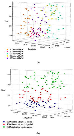
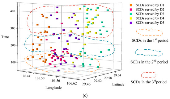
Figure 8.
Clustering results of SCDs by improved k-medoids in a collaborative network. (a) SCDs in different depots; (b) SCDs in different service periods; (c) SCDs in different depots and service periods.
In Figure 8a, the SCDs are grouped into five and reassigned to the nearest depot according to the temporal–spatial distance between each medoid and each depot. In Figure 8b, three service periods are determined by clustering results. In Figure 8c, each SCD is assigned to each depot for each service period. The clustering results of SCDs and DCDs are presented in Figure 9.
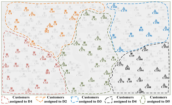
Figure 9.
Clustering results of DCDs based on geographical location.
Figure 9 is divided into five parts, indicating the service areas of each of the five depots. The DCDs with similar geographical locations are assigned to the same depot in the collaborative network to reduce long-distance transportation and cross-transportation routes. Then, the vehicle routes between depots and customers can be optimized using IMOPSO-DIS for each clustering unit.
5.2.3. Results of Routing Optimization with Resource Sharing and DIS
Resource sharing and the DIS adopted in collaborative logistics networks optimize the vehicle scheduling and routing among multiple depots. The vehicle routes are determined with minimum TOC and NV through the IMOPSO-DIS algorithm introduced in Section 4.2. According to related research [93,94] and the scale of real-world logistics networks, the parameters in the proposed model and algorithm can be set, as shown in Table 7. The initial vehicle routes without resource sharing and DIS in the initial network are presented in Figure 10.
Table 7.
Definitions and values of parameters considered in the proposed model and algorithm.
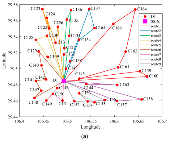
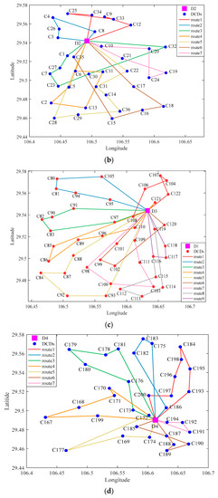
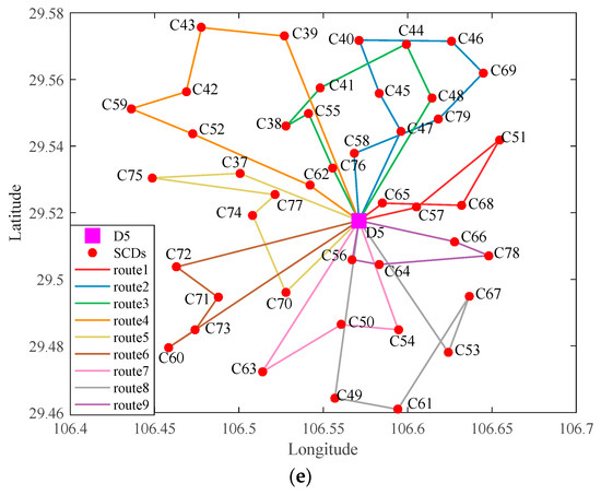
Figure 10.
Initial routes without resource sharing and DIS in noncollaborative MVRPDCDTW. (a) Initial vehicle routes of D1; (b) Initial vehicle routes of D2; (c) Initial vehicle routes of D3; (d) Initial vehicle routes of D4; (e) Initial vehicle routes of D5.
In Figure 10, SCDs and DCDs are served independently by each depot in noncollaborative MVRPDCDTW. In Figure 10a–e, the red pots, blue pots, and squares refer to SCDs, DCDs, and depots. D1, D2, D3, D4, and D5 have 9, 7, 9, 7, and 9 delivery routes, respectively, where D1, D3, and D5 serve SCDs and D2 and D4 serve DCDs. The results in the initial network are shown in Table 8.
Table 8.
Results in the noncollaborative logistics network.
In Table 8, the results in the noncollaborative logistics network comprise DC, PC, MC, FC, and NV of each depot. The maximum TOC of D1 is $13,872.65, and the minimum total cost of D4 is $10,937.18. The TOC and NV in the noncollaborative logistics network are $62,011.18 and 41. However, the TRS and DIS are introduced to optimize CMVRPDCDTW and coordinate SCDs and DCDs. Table 9 lists the optimized results of multiple depots in three service periods.
Table 9.
Optimized results of multidepot network in three service periods.
Various costs of each depot and the number of routes of each depot in three service periods are presented in Table 9. The total DC, total PC, and total IC in the optimized collaborative networks are $28,475.98, $1509.61, and $6400, respectively. The total number of routes of the five depots is 33. Table 10 presents the specific optimized vehicle routes with DIS in CMVRPDCDTW.
Table 10.
Optimized vehicle routes with DIS in CMVRPDCDTW.
In Table 10, the number of routes in D1, D2, D3, D4, and D5 is 8, 7, 6, 5, and 7, respectively. The vehicle routes optimized through DIS can be divided into three types: pure static routes where the demands on the route are static (i.e., R8); pure dynamic routes where the demands on the route are dynamic (i.e., R21); mixed route where the demands on the route are composed of SCDs and DCDs (i.e., R1). The mixed routes generated by inserted DCDs into pure statics routes make full use of the remaining capacity of vehicles, thereby improving the utilization of resources and decreasing the TOC. The comparison of vehicle routes of D4 and D5 without and with DIS is shown in Figure 11.

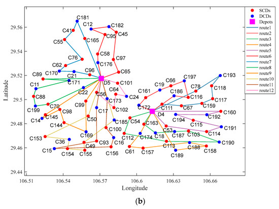
Figure 11.
Comparison of vehicle routes of D4 and D5 without and with DIS. (a) Vehicle routes of D4 and D5 without DIS; (b) Vehicle routes of D5 and D4 with DIS.
In Figure 11a, the DCDs are visited by new vehicles, in particular, the depots dispatch new vehicles to serve DCDs alone when DCDs appear. For example, routes 1–7 and routes 14–18 are planned at first for SCDs, and then when DCDs appear, the new vehicles are dispatched to travel routes 8–13 and 19–22 for DCDs. However, as shown in Figure 11b, the SCDs and DCDs are coordinated to generate mixed routes by implementing the DIS, thereby reducing the number of routes from 22 to 12. For instance, SCDs (C14 *, C169 *) are inserted in a suitable position on the route D5→C145→C98→C144→C99→D1 to generate the mixed route D5→C145→C14 *→C98→C144→C169 *→C99→D1. The TOC including TC, DC, PC, IC, FC, MC, NST, and NV before and after CMVRPDCDTW optimization are shown in Table 11 and Figure 12.
Table 11.
Result comparison before and after CMVRPDCDTW optimization.
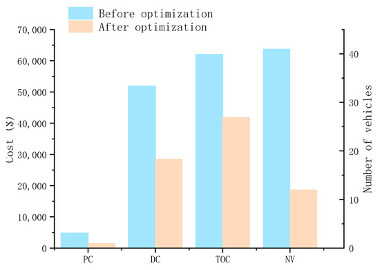
Figure 12.
Comparison before and after CMVRPDCDTW optimization.
In Table 11, the TC and NST are added to $5147.36 and one because of the transfer of goods among depots. Meanwhile, the IC increased by $6400 because of the implementation of DIS. However, the TOC is decreased by $20,138.21 from $62,011.18 to $41,872.97, and the NV saves 29 after optimization. Compared with the initial logistics network, the PC, DC, TOC, and NV in the optimized network are decreased to some extent, as shown in Figure 12. Accordingly, the proposed model and algorithm are effective for CMVRPDCDTW optimization.
5.3. Analysis and Discussion
5.3.1. Results of Different Numbers of Service Periods
The four scenarios are designed to determine the optimal number of service periods for this real logistics network. The working periods of depots are divided into two, three, and four service periods and compared with one service period to explore the effect of the different numbers of service periods on the optimization results. If the time windows of the depots are [0, T], then the working periods of depots can be divided into r service periods, and the length of each is tn = T/r. The specific time windows of each service period can be divided into four cases by setting T = 24, as shown in Table 12. The optimized results including TOC and NV, of the four scenarios, are shown in Table 13 and Figure 13.
Table 12.
Time windows determination in five cases.
Table 13.
Optimization results for the four scenarios.

Figure 13.
Optimization results for different r values.
Table 13 and Figure 13 demonstrate the TOC and NV in different values of r. Compared with the TOCs in the other three scenarios, the TOC when r = 3 is minimized to $41,872.97, which is a reduction of $11,856.87, $2251.02, and $4612.62. Compared with the NV in the first scenario, the NV considerably declines after vehicle sharing among multiple service periods, saving 18, 26, and 29 when r = 2, r = 3, and r = 4. In the latter two cases, the change in the NV is relatively flat compared with that in the TOC. Therefore, the working period of depots is divided into three in this study to minimize the TOC and NV.
5.3.2. Results of Different Optimization Strategies
In this section, four cases are designed to analyze the influence of collaborative mode and DIS on optimization results to verify the performance of optimization strategy on CMVRPDCDTW optimization. Case 1: resource sharing and DIS are not considered in the optimization process; Case 2: CSS is adopted based on Case 1. Case 3: CSS and TRS are shared among depots but DIS is not employed. Case 4: the DIS is adopted based on Case 3. The optimization results of four cases are given in Table 14 and Figure 14.
Table 14.
Optimization results of four cases.
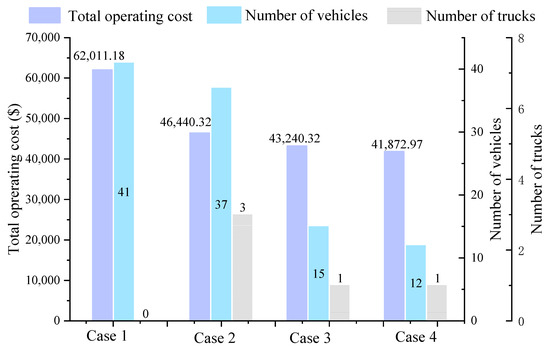
Figure 14.
Comparison of optimized results in four cases.
Table 14 shows the optimization results of the four cases including three items, namely, TOC, NV, and NST. The TOC of the four cases are $62,011.18, $46,440.32, $43,240.32, and $41,872.97. The NVs of the four cases are 41, 37, 15, and 12. The NSTs of the four cases are 0, 3, 1, and 1.
In Figure 14, the optimized results of Case 1 and Case2 indicate that the CSS among depots can save TOC by reducing the travel distance and violations of time windows. The TRS contributes to the reduction of the NV and NST by comparing Case 2 with Case 3. Compared with the TOC and NV in other cases, the TOC and NV when the DIS is adopted in Case 4 are decreased. Accordingly, the collaborative mode and DIS help save the TOC and NV in CMVRPDCDTW.
The effects of different service periods (i.e., r = 1, r = 2, r = 3, and r = 4) and optimization strategies (CSS, TRS, and DIS) on vehicle routing results are analyzed and discussed in this section. The service periods are divided into four scenarios, and then the TOC and NV in each service period are calculated. The r = 3 is determined as the most appropriate number of service periods by comparing the calculated results of four scenarios. Moreover, the different optimization strategies are adopted in four cases, the results reveal that the TOC and NV are gradually reduced as optimization strategies are implemented. Therefore, different service periods and optimization strategies can provide enterprises with deep management practices and methods for reference.
5.4. Management Insights
In this study, resource sharing and dynamic insertion strategies are adopted to optimize CMVRPDCDTW by considering logistics resource configuration and delivery route planning in multiple service periods. The optimization strategies provide relevant managerial implications for logistics service providers to implement vehicle scheduling and route planning in a collaborative multidepot distribution network with DCDs, which can be summarized in the following three aspects.
The proposed bi-objective optimization model and solution methodology offer a reference for decision makers to optimize delivery routes and vehicle scheduling in a dynamic environment. On the one hand, the TOC and NV, regarded as valued optimization goals by logistics enterprises, are simultaneously considered in the model. On the other hand, the application of the proposed IMOPSO-DIS algorithm optimizes the delivery routes by inserting the DCDs in the existing routes to obtain high-quality solutions, thereby improving the company’s responsiveness to distribution networks with DCDs.
The new customer demands occurring in the delivery logistics network present new challenges for reasonable delivery route planning and vehicle scheduling among multiple depots. The introduction of DIS can readjust vehicle routes when new customer demands appear. This strategy can provide a relatively optimal delivery scheme to enhance the responsiveness of the logistics distribution system with the DCDs, thereby ensuring service quality and improving operational efficiency. Accordingly, the collaborative mode and DIS should be developed by logistics service providers to solve the CMVRPDCDTW.
A growing number of platforms and new technologies are emerging to support collaborative transportation systems by enabling real-time information sharing and carrier interaction. Logistics decision makers should explore various effective collaboration modes adapted to their business development to increase market competitiveness. Customers in a collaborative logistics network are reassigned to the nearest depot based on temporal–spatial distances. This scenario helps reduce travel distances and improve the operational efficiency of the distribution logistics network. Meanwhile, the delivery vehicles can be shared in multiple service periods to improve transportation resource utilization. Therefore, designing a collaborative distribution logistics network can reduce the TOC and NV, thereby promoting the sustainable development of urban transportation systems.
6. Conclusions
Collaboration has been proved to be an effective method for improving transportation efficiency by resource sharing among participants over multiple service periods. This method can reduce DCs and maximize resource utilization. This research proposes and solves a collaborative MDVRP formulated as a bi-objective CMVRPDCDTW optimization model by considering time windows and DCDs. The improved k-medoids clustering algorithm is designed to divide the service areas for depots based on the time windows and customer geographical locations. The IMOPSO-DIS algorithm is devised to optimize vehicle routing with minimum TOC and NV for the CMVRPDCDTW. The DIS is utilized in this algorithm to adjust the optimal delivery solutions and respond to DCDs.
A real-world case study is implemented in a multidepot logistics network in Chongqing City, China to evaluate the effectiveness of the proposed optimization model and solution methodology. The comparison of the results before and after optimization reveals that the TOC is reduced to $41,872.97, achieving a savings of 32.5%. Moreover, the NV is decreased to 12 after the application of optimization strategies. Different service periods and optimization strategies are further discussed and analyzed. The results show that r = 3 is the optimal number of service periods for the logistics network designed in this study. The application of CSS, TRS, and DIS in distribution logistics networks with DCDs can reduce TOCs and achieve the appropriate configuration of logistics resources. This scenario contributes to the establishment of a sustainable and economical urban distribution system.
This study investigates the widespread presence of DCDs in today’s logistics networks and incorporates the dynamic characteristics into a real-time vehicle routing optimization process in a logistics network. Compared with the traditional network optimization (i.e., the network optimization with SCDs), the integration of DCDs and SCDs enables the proposed CMVRPDCDTW optimization to better satisfy the increasingly vital requirements of high-flexibility in vehicle scheduling for modern logistics enterprises. At present, the ubiquity of various new technologies such as blockchain, cloud computing, and big data has deeply penetrated into modern logistics operations. Combined with the collaborative strategies and the DIS method, the proposed model and algorithm can effectively handle the collected dynamic customer information and provide logistics managers with timely vehicle scheduling adjustment and optimization, thus accelerating the flexible development of sustainable logistics systems.
Future studies have some room for improvement. (1) This research can be extended to different realistic network dynamic scenarios, such as variable customer time windows and traffic congestion. (2) The pickup and delivery operations can be simultaneously considered in optimizing the multidepot delivery logistics networks. (3) Exact algorithms can combine with heuristic algorithms in future studies to improve solution quality. (4) The optimization objectives (e.g., environmental factors, social impact, enterprise benefits, and customer satisfaction) can be considered in the CMVRPDCDTW model.
Author Contributions
Conceptualization, Y.W. and J.Z.; methodology, Y.W. and J.Z.; software, J.Z.; validation, J.Z. and X.W.; formal analysis, Y.W. and J.Z.; investigation, J.Z., X.W. and Y.S.; resources, Y.W.; data curation, Y.W. and J.Z.; writing—original draft preparation, Y.W. and J.Z.; writing—review and editing, Y.W., J.Z., X.W., Y.S. and H.W.; visualization, J.Z. and X.W.; supervision, Y.W. and H.W.; project administration, Y.W.; funding acquisition, Y.W. All authors have read and agreed to the published version of the manuscript.
Funding
The authors would like to express our sincere appreciation for the valuable comments made by three anonymous reviewers, which helped us to improve the quality of this paper. This research is supported by National Natural Science Foundation of China (71871035), Key Science and Technology Research Project of Chongqing Municipal Education Commission (KJZD-K202000702), Key Project of Human Social Science of Chongqing Municipal Education Commission (20SKGH079), Chongqing Liuchuang Plan Innovation Project (cx2021038), Team Building Project for Graduate Tutors in Chongqing (JDDSTD2019008), Chongqing Bayu Scholar Youth Project (YS2021058).
Institutional Review Board Statement
Not applicable.
Informed Consent Statement
Not applicable.
Data Availability Statement
Not applicable.
Conflicts of Interest
The authors declare no conflict of interest.
References
- Bent, R.W.; Van Hentenryck, P. Scenario-based planning for partially dynamic vehicle routing with stochastic customers. Oper. Res. 2004, 52, 977–987. [Google Scholar] [CrossRef] [Green Version]
- Mańdziuk, J.; Żychowski, A. A memetic approach to vehicle routing problem with dynamic requests. Appl. Soft Comput. 2016, 48, 522–534. [Google Scholar] [CrossRef]
- Ahkamiraad, A.; Wang, Y. Capacitated and multiple cross-docked vehicle routing problem with pickup, delivery, and time windows. Comput. Ind. Eng. 2018, 119, 76–84. [Google Scholar] [CrossRef]
- Bettinelli, A.; Ceselli, A.; Righini, G. A branch-and-cut-and-price algorithm for the multi-depot heterogeneous vehicle routing problem with time windows. Transp. Res. Part C Emerg. Technol. 2011, 19, 723–740. [Google Scholar] [CrossRef]
- Sadati, M.E.H.; Çatay, B. A hybrid variable neighborhood search approach for the multi-depot green vehicle routing problem. Transp. Res. Part E Logist. Transp. Rev. 2021, 149, 102293. [Google Scholar] [CrossRef]
- Wang, S.H.; Han, C.; Yu, Y.; Huang, M.; Sun, W.; Kaku, I. Reducing carbon emissions for the vehicle routing problem by utilizing multiple depots. Sustainability 2022, 14, 1264. [Google Scholar] [CrossRef]
- Xu, Z.T.; Elomri, A.; Pokharel, S.; Mutlu, F. A model for capacitated green vehicle routing problem with the time-varying vehicle speed and soft time windows. Comput. Ind. Eng. 2019, 137, 106011. [Google Scholar] [CrossRef]
- Li, J.Q.; Han, Y.Q.; Duan, P.Y.; Han, Y.Y.; Niu, B.; Li, C.D.; Zheng, Z.X.; Liu, Y.P. Meta-heuristic algorithm for solving vehicle routing problems with time windows and synchronized visit constraints in prefabricated systems. J. Clean. Prod. 2020, 250, 119464. [Google Scholar] [CrossRef]
- Bae, H.; Moon, I. Multi-depot vehicle routing problem with time windows considering delivery and installation vehicles. Appl. Math. Model. 2016, 40, 6536–6549. [Google Scholar] [CrossRef]
- Fan, H.; Zhang, Y.G.; Tian, P.J.; Lv, Y.C.; Fan, H. Time-dependent multi-depot green vehicle routing problem with time windows considering temporal-spatial distance. Comput. Oper. Res. 2021, 129, 105211. [Google Scholar] [CrossRef]
- Dayarian, I.; Crainic, T.G.; Gendreau, M.; Rei, W. An adaptive large-neighborhood search heuristic for a multi-period vehicle routing problem. Transp. Res. Part E Logist. Transp. Rev. 2016, 95, 95–123. [Google Scholar] [CrossRef]
- Wang, Y.; Li, Q.; Guan, X.Y.; Xu, M.Z.; Liu, Y.; Wang, H.Z. Two-echelon collaborative multi-depot multi-period vehicle routing problem. Expert Syst. Appl. 2021, 167, 114201. [Google Scholar] [CrossRef]
- Kuo, R.J.; Wibowo, B.S.; Zulvia, F.E. Application of a fuzzy ant colony system to solve the dynamic vehicle routing problem with uncertain service time. Appl. Math. Model. 2016, 40, 9990–10001. [Google Scholar] [CrossRef]
- Zhang, J.L.; Lam, W.H.K.; Chen, B.Y. On-time delivery probabilistic models for the vehicle routing problem with stochastic demands and time windows. Eur. J. Oper. Res. 2016, 249, 144–154. [Google Scholar] [CrossRef]
- Wang, Y.; Ran, L.Y.; Guan, X.Y.; Fan, J.X.; Sun, Y.Y.; Wang, H.Z. Collaborative multicenter vehicle routing problem with time windows and mixed deliveries and pickups. Expert Syst. Appl. 2022, 197, 116690. [Google Scholar] [CrossRef]
- Albareda-Sambola, M.; Fernández, E.; Laporte, G. The dynamic multiperiod vehicle routing problem with probabilistic information. Comput. Oper. Res. 2014, 48, 31–39. [Google Scholar] [CrossRef]
- Sarasola, B.; Doerner, K.F.; Schmid, V.; Alba, E. Variable neighborhood search for the stochastic and dynamic vehicle routing problem. Ann. Oper. Res. 2015, 236, 425–461. [Google Scholar] [CrossRef]
- Xu, H.T.; Pu, P.; Duan, F. Dynamic Vehicle Routing Problems with Enhanced Ant Colony Optimization. Discret. Dyn. Nat. Soc. 2018, 2018, 1–13. [Google Scholar] [CrossRef] [Green Version]
- Los, J.; Schulte, F.; Spaan, M.T.J.; Negenborn, R.R. The value of information sharing for platform-based collaborative vehicle routing. Transp. Res. Part E Logist. Transp. Rev. 2020, 141, 102011. [Google Scholar] [CrossRef]
- Wang, Y.; Li, Q.; Guan, X.Y.; Fan, J.X.; Liu, Y.; Wang, H.Z. Collaboration and resource sharing in the multidepot multiperiod vehicle routing problem with pickups and deliveries. Sustainability 2020, 12, 5966. [Google Scholar] [CrossRef]
- Chakraborty, D.; Garai, T.; Jana, D.K.; Roy, T.K. A three-layer supply chain inventory model for non-instantaneous deteriorating item with inflation and delay in payments in random fuzzy environment. J. Ind. Prod. Eng. 2017, 34, 407–424. [Google Scholar] [CrossRef]
- Paul, A.; Garai, T.; Giri, B. Sustainable supply chain coordination with greening and promotional effort dependent demand. Int. J. Procure. Manag. 2021, in press. [Google Scholar] [CrossRef]
- Xiang, X.S.; Qiu, J.F.; Xiao, J.H.; Zhang, X.Y. Demand coverage diversity based ant colony optimization for dynamic vehicle routing problems. Eng. Appl. Artif. Intell. 2020, 91, 103582. [Google Scholar] [CrossRef]
- Niu, Y.Y.; Zhang, Y.P.; Cao, Z.G.; Gao, K.Z.; Xiao, J.H.; Song, W.; Zhang, F.W. MIMOA: A membrane-inspired multi-objective algorithm for green vehicle routing problem with stochastic demands. Swarm Evol. Comput. 2021, 60, 100767. [Google Scholar] [CrossRef]
- Park, H.S.; Jun, C.H. A simple and fast algorithm for K-medoids clustering. Expert Syst. Appl. 2009, 36, 3336–3341. [Google Scholar] [CrossRef]
- Wang, Y.; Sun, Y.Y.; Guan, X.Y.; Fan, J.X.; Xu, M.Z.; Wang, H.Z. Two-echelon multi-period location routing problem with shared transportation resource. Knowl. -Based Syst. 2021, 226, 107168. [Google Scholar] [CrossRef]
- Hanshar, F.T.; Ombuki-Berman, B.M. Dynamic vehicle routing using genetic algorithms. Appl. Intell. 2007, 27, 89–99. [Google Scholar] [CrossRef]
- Xu, H.T.; Pu, P.; Duan, F. A hybrid ant colony optimization for dynamic multidepot vehicle routing problem. Discret. Dyn. Nat. Soc. 2018, 2018, 1–10. [Google Scholar] [CrossRef] [Green Version]
- Okulewicz, M.; Mańdziuk, J. The impact of particular components of the PSO-based algorithm solving the Dynamic Vehicle Routing Problem. Appl. Soft Comput. 2017, 58, 586–604. [Google Scholar] [CrossRef]
- Hong, L.X. An improved LNS algorithm for real-time vehicle routing problem with time windows. Comput. Oper. Res. 2012, 39, 151–163. [Google Scholar] [CrossRef]
- Barkaoui, M.; Berger, J.; Boukhtouta, A. Customer satisfaction in dynamic vehicle routing problem with time windows. Appl. Soft Comput. 2015, 35, 423–432. [Google Scholar] [CrossRef]
- Goel, R.; Maini, R.; Bansal, S. Vehicle routing problem with time windows having stochastic customer demands and stochastic service times: Modelling and solution. J. Comput. Sci. 2019, 34, 1–10. [Google Scholar] [CrossRef]
- Errico, F.; Desaulniers, G.; Gendreau, M.; Rei, W.; Rousseau, L.M. The vehicle routing problem with hard time windows and stochastic service times. EURO J. Transp. Logist. 2018, 7, 223–251. [Google Scholar] [CrossRef]
- Basso, R.; Kulcsár, B.; Sanchez-Diaz, I.; Qu, X.B. Dynamic stochastic electric vehicle routing with safe reinforcement learning. Transp. Res. Part E Logist. Transp. Rev. 2022, 157, 102496. [Google Scholar] [CrossRef]
- Carrese, S.; Cipriani, E.; Mannini, L.; Nigro, M. Dynamic demand estimation and prediction for traffic urban networks adopting new data sources. Transp. Res. Part C Emerg. Technol. 2017, 81, 83–98. [Google Scholar] [CrossRef]
- Roy, K.C.; Hasan, S.; Culotta, A.; Eluru, N. Predicting traffic demand during hurricane evacuation using Real-time data from transportation systems and social media. Transp. Res. Part C Emerg. Technol. 2021, 131, 103339. [Google Scholar] [CrossRef]
- Huang, F.H.; Yi, P.Y.; Wang, J.C.; Li, M.S.; Peng, J.; Xiong, X. A dynamical spatial-temporal graph neural network for traffic demand prediction. Inf. Sci. 2022, 594, 286–304. [Google Scholar] [CrossRef]
- Jie, K.W.; Liu, S.Y.; Sun, X.J. A hybrid algorithm for time-dependent vehicle routing problem with soft time windows and stochastic factors. Eng. Appl. Artif. Intell. 2022, 109, 104606. [Google Scholar] [CrossRef]
- Peled, I.; Lee, K.; Jiang, Y.; Dauwels, J.; Pereira, F.C. On the quality requirements of demand prediction for dynamic public transport. Commun. Transp. Res. 2021, 1, 100008. [Google Scholar] [CrossRef]
- Chen, S.F.; Chen, R.; Wang, G.G.; Gao, J.; Sangaiah, A.K. An adaptive large neighborhood search heuristic for dynamic vehicle routing problems. Comput. Electr. Eng. 2018, 67, 596–607. [Google Scholar] [CrossRef]
- Laganà, D.; Laporte, G.; Vocaturo, F. A dynamic multi-period general routing problem arising in postal service and parcel delivery systems. Comput. Oper. Res. 2021, 129, 105195. [Google Scholar] [CrossRef]
- Xue, G.Q.; Wang, Y.; Guan, X.Y.; Wang, Z. A combined GA-TS algorithm for two-echelon dynamic vehicle routing with proactive satellite stations. Comput. Ind. Eng. 2022, 164, 107899. [Google Scholar] [CrossRef]
- Li, J.; Wang, R.; Li, T.T.; Lu, Z.X.; Pardalos, P.M. Benefit analysis of shared depot resources for multi-depot vehicle routing problem with fuel consumption. Transp. Res. Part D Transp. Environ. 2018, 59, 417–432. [Google Scholar] [CrossRef]
- Soeanu, A.; Ray, S.; Berger, J.; Boukhtouta, A.; Debbabi, M. Multi-depot vehicle routing problem with risk mitigation: Model and solution algorithm. Expert Syst. Appl. 2020, 145, 113099. [Google Scholar] [CrossRef]
- Wang, X.P.; Lin, N.; Li, Y.; Shi, Y.; Ruan, J.H. An integrated modeling method for collaborative vehicle routing: Facilitating the unmanned micro warehouse pattern in new retail. Expert Syst. Appl. 2021, 168, 114307. [Google Scholar] [CrossRef]
- Zhen, L.; Ma, C.L.; Wang, K.; Xiao, L.Y.; Zhang, W. Multi-depot multi-trip vehicle routing problem with time windows and release dates. Transp. Res. Part E Logist. Transp. Rev. 2020, 135, 101866. [Google Scholar] [CrossRef]
- Sadati, M.E.H.; Çatay, B.; Aksen, D. An efficient variable neighborhood search with tabu shaking for a class of multi-depot vehicle routing problems. Comput. Oper. Res. 2021, 133, 105269. [Google Scholar] [CrossRef]
- Yang, F.; Dai, Y.; Ma, Z.J. A cooperative rich vehicle routing problem in the last-mile logistics industry in rural areas. Transp. Res. Part E Logist. Transp. Rev. 2020, 141, 102024. [Google Scholar] [CrossRef]
- Mancini, S.; Gansterer, M.; Hartl, R.F. The collaborative consistent vehicle routing problem with workload balance. Eur. J. Oper. Res. 2021, 293, 955–965. [Google Scholar] [CrossRef]
- Wang, Y.; Wang, X.W.; Guan, X.Y.; Li, Q.; Fan, J.X.; Wang, H.Z. A combined intelligent and game theoretical methodology for collaborative multicenter pickup and delivery problems with time window assignment. Appl. Soft Comput. 2021, 113, 107875. [Google Scholar] [CrossRef]
- Qin, X.R.; Yang, H.; Wu, Y.H.; Zhu, H.T. Multi-party ride-matching problem in the ride-hailing market with bundled option services. Transp. Res. Part C Emerg. Technol. 2021, 131, 103287. [Google Scholar] [CrossRef]
- Gao, J.; Li, S.; Yang, H. Shared parking for ride-sourcing platforms to reduce cruising traffic. Transp. Res. Part C Emerg. Technol. 2022, 137, 103562. [Google Scholar] [CrossRef]
- Wei, S.Q.; Feng, S.Y.; Ke, J.T.; Yang, H. Calibration and validation of matching functions for ride-sourcing markets. Commun. Transp. Res. 2022, 2, 100058. [Google Scholar] [CrossRef]
- Muñoz-Villamizar, A.; Montoya-Torres, J.R.; Faulin, J. Impact of the use of electric vehicles in collaborative urban transport networks: A case study. Transp. Res. Part D Transp. Environ. 2017, 50, 40–54. [Google Scholar] [CrossRef]
- Vaziri, S.; Etebari, F.; Vahdani, B. Development and optimization of a horizontal carrier collaboration vehicle routing model with multi-commodity request allocation. J. Clean. Prod. 2019, 224, 492–505. [Google Scholar] [CrossRef]
- Zhang, Q.H.; Wang, Z.T.; Huang, M.; Yu, Y.; Fang, S.C. Heterogeneous multi-depot collaborative vehicle routing problem. Transp. Res. Part B Methodol. 2022, 160, 1–20. [Google Scholar] [CrossRef]
- Mancini, S. A real-life multi depot multi period vehicle routing problem with a heterogeneous fleet: Formulation and adaptive large neighborhood search based matheuristic. Transp. Res. Part C Emerg. Technol. 2016, 70, 100–112. [Google Scholar] [CrossRef]
- Ting, C.K.; Liao, X.L.; Huang, Y.H.; Liaw, R.T. Multi-vehicle selective pickup and delivery using metaheuristic algorithms. Inf. Sci. 2017, 406–407, 146–169. [Google Scholar] [CrossRef]
- Liu, R.; Jiang, Z. A hybrid large-neighborhood search algorithm for the cumulative capacitated vehicle routing problem with time-window constraints. Appl. Soft Comput. 2019, 80, 18–30. [Google Scholar] [CrossRef]
- Lin, C.K.Y. A cooperative strategy for a vehicle routing problem with pickup and delivery time windows. Comput. Ind. Eng. 2008, 55, 766–782. [Google Scholar] [CrossRef]
- Ghannadpour, S.F.; Noori, S.; Tavakkoli-Moghaddam, R.; Ghoseiri, K. A multi-objective dynamic vehicle routing problem with fuzzy time windows: Model, solution and application. Appl. Soft Comput. 2014, 14, 504–527. [Google Scholar] [CrossRef]
- Li, J.; Li, Y.; Pardalos, P.M. Multi-depot vehicle routing problem with time windows under shared depot resources. J. Comb. Optim. 2014, 31, 515–532. [Google Scholar] [CrossRef]
- Fernández, E.; Roca-Riu, M.; Speranza, M.G. The Shared Customer Collaboration Vehicle Routing Problem. Eur. J. Oper. Res. 2018, 265, 1078–1093. [Google Scholar] [CrossRef] [Green Version]
- Li, Y.B.; Soleimani, H.; Zohal, M. An improved ant colony optimization algorithm for the multi-depot green vehicle routing problem with multiple objectives. J. Clean. Prod. 2019, 227, 1161–1172. [Google Scholar] [CrossRef]
- Zhang, W.Y.; Chen, Z.X.; Zhang, S.; Wang, W.R.; Yang, S.Q.; Cai, Y.S. Composite multi-objective optimization on a new collaborative vehicle routing problem with shared carriers and depots. J. Clean. Prod. 2020, 274, 122593. [Google Scholar] [CrossRef]
- Wang, F.; Liao, F.S.; Li, Y.X.; Yan, X.S.; Chen, X. An ensemble learning based multi-objective evolutionary algorithm for the dynamic vehicle routing problem with time windows. Comput. Ind. Eng. 2021, 154, 107131. [Google Scholar] [CrossRef]
- Khouadjia, M.R.; Sarasola, B.; Alba, E.; Jourdan, L.; Talbi, E.G. A comparative study between dynamic adapted PSO and VNS for the vehicle routing problem with dynamic requests. Appl. Soft Comput. 2012, 12, 1426–1439. [Google Scholar] [CrossRef]
- Abdallah, A.M.F.M.; Essam, D.L.; Sarker, R.A. On solving periodic re-optimization dynamic vehicle routing problems. Appl. Soft Comput. 2017, 55, 1–12. [Google Scholar] [CrossRef]
- Ganji, M.; Kazemipoor, H.; Molana, S.M.H.; Sajadi, S.M. A green multi-objective integrated scheduling of production and distribution with heterogeneous fleet vehicle routing and time windows. J. Clean. Prod. 2020, 259, 120824. [Google Scholar] [CrossRef]
- Kumar, R.S.; Kondapaneni, K.; Dixit, V.; Goswami, A.; Thakur, L.S.; Tiwari, M.K. Multi-objective modeling of production and pollution routing problem with time window: A self-learning particle swarm optimization approach. Comput. Ind. Eng. 2016, 99, 29–40. [Google Scholar] [CrossRef]
- Srivastava, G.; Singh, A.; Mallipeddi, R. NSGA-II with objective-specific variation operators for multiobjective vehicle routing problem with time windows. Expert Syst. Appl. 2021, 176, 114779. [Google Scholar] [CrossRef]
- Zhang, W.Q.; Yang, D.J.; Zhang, G.H.; Gen, M. Hybrid multiobjective evolutionary algorithm with fast sampling strategy-based global search and route sequence difference-based local search for VRPTW. Expert Syst. Appl. 2020, 145, 113151. [Google Scholar] [CrossRef]
- Niu, Y.Y.; Kong, D.; Wen, R.; Cao, Z.G.; Xiao, J.H. An improved learnable evolution model for solving multi-objective vehicle routing problem with stochastic demand. Knowl. -Based Syst. 2021, 230, 107378. [Google Scholar] [CrossRef]
- Zarouk, Y.; Mahdavi, I.; Rezaeian, J.; Santos-Arteaga, F.J. A novel multi-objective green vehicle routing and scheduling model with stochastic demand, supply, and variable travel times. Comput. Oper. Res. 2022, 141, 105698. [Google Scholar] [CrossRef]
- Eskandarpour, M.; Ouelhadj, D.; Hatami, S.; Juan, A.A.; Khosravi, B. Enhanced multi-directional local search for the bi-objective heterogeneous vehicle routing problem with multiple driving ranges. Eur. J. Oper. Res. 2019, 277, 479–491. [Google Scholar] [CrossRef]
- Asadi, E.; Habibi, F.; Nickel, S.; Sahebi, H. A bi-objective stochastic location-inventory-routing model for microalgae-based biofuel supply chain. Appl. Energy 2018, 228, 2235–2261. [Google Scholar] [CrossRef]
- Farham, M.S.; Süral, H.; Iyigun, C. A column generation approach for the location-routing problem with time windows. Comput. Oper. Res. 2018, 90, 249–263. [Google Scholar] [CrossRef]
- Mokhtarzadeh, M.; Tavakkoli-Moghaddam, R.; Triki, C.; Rahimi, Y. A hybrid of clustering and meta-heuristic algorithms to solve a p-mobile hub location–allocation problem with the depreciation cost of hub facilities. Eng. Appl. Artif. Intell. 2021, 98, 104121. [Google Scholar] [CrossRef]
- Lyu, Y.; Chow, C.Y.; Lee VC, S.; Ng JK, Y.; Li, Y.H.; Zeng, J. CB-Planner: A bus line planning framework for customized bus systems. Transp. Res. Part C Emerg. Technol. 2019, 101, 233–253. [Google Scholar] [CrossRef]
- Rabbani, M.; Heidari, R.; Farrokhi-Asl, H.; Rahimi, N. Using metaheuristic algorithms to solve a multi-objective industrial hazardous waste location-routing problem considering incompatible waste types. J. Clean. Prod. 2018, 170, 227–241. [Google Scholar] [CrossRef]
- Rezaei, M.; Afsahi, M.; Shafiee, M.; Patriksson, M. A bi-objective optimization framework for designing an efficient fuel supply chain network in post-earthquakes. Comput. Ind. Eng. 2020, 147, 106654. [Google Scholar] [CrossRef]
- Eberhart, R.; Kennedy, J. A new optimizer using particle swarm theory. In MHS’95, Proceedings of the Sixth International Symposium on Micro Machine and Human Science, Nagoya, Japan, 4–6 October 1995; IEEE: Piscataway, NJ, USA, 1995; pp. 39–43. [Google Scholar]
- Coello, C.A.C.; Pulido, G.T.; Lechuga, M.S. Handling multiple objectives with particle swarm optimization. IEEE Trans. Evol. Comput. 2004, 8, 256–279. [Google Scholar] [CrossRef]
- Moslemi, H.; Zandieh, M. Comparisons of some improving strategies on MOPSO for multi-objective (r,Q) inventory system. Expert Syst. Appl. 2011, 38, 12051–12057. [Google Scholar] [CrossRef]
- Li, L.; Li, G.P.; Chang, L. A many-objective particle swarm optimization with grid dominance ranking and clustering. Appl. Soft Comput. 2020, 96, 106661. [Google Scholar] [CrossRef]
- Govindan, K.; Jafarian, A.; Khodaverdi, R.; Devika, K. Two-echelon multiple-vehicle location–routing problem with time windows for optimization of sustainable supply chain network of perishable food. Int. J. Prod. Econ. 2014, 152, 9–28. [Google Scholar] [CrossRef]
- Lim, W.H.; Isa, N.A.M. An adaptive two-layer particle swarm optimization with elitist learning strategy. Inf. Sci. 2014, 273, 49–72. [Google Scholar] [CrossRef]
- Ding, S.X.; Chen, C.; Xin, B.; Pardalos, P.M. A bi-objective load balancing model in a distributed simulation system using NSGA-II and MOPSO approaches. Appl. Soft Comput. 2018, 63, 249–267. [Google Scholar] [CrossRef]
- Renaud, J.; Boctor, F.F.; Ouenniche, J. A heuristic for the pickup and delivery traveling salesman problem. Comput. Oper. Res. 2000, 27, 905–916. [Google Scholar] [CrossRef]
- Rashidnejad, M.; Ebrahimnejad, S.; Safari, J. A bi-objective model of preventive maintenance planning in distributed systems considering vehicle routing problem. Comput. Ind. Eng. 2018, 120, 360–381. [Google Scholar] [CrossRef]
- Lin, Q.Z.; Li, J.Q.; Du, Z.H.; Chen, J.Y.; Ming, Z. A novel multi-objective particle swarm optimization with multiple search strategies. Eur. J. Oper. Res. 2015, 247, 732–744. [Google Scholar] [CrossRef]
- Yang, S.X.; Jiang, S.Y.; Jiang, Y. Improving the multiobjective evolutionary algorithm based on decomposition with new penalty schemes. Soft Comput. 2016, 21, 4677–4691. [Google Scholar] [CrossRef] [Green Version]
- Ghodratnama, A.; Jolai, F.; Tavakkoli-Moghaddam, R. Solving a new multi-objective multi-route flexible flow line problem by multi-objective particle swarm optimization and NSGA-II. J. Manuf. Syst. 2015, 36, 189–202. [Google Scholar] [CrossRef]
- Abad, H.K.E.; Vahdani, B.; Sharifi, M.; Etebari, F. A bi-objective model for pickup and delivery pollution-routing problem with integration and consolidation shipments in cross-docking system. J. Clean. Prod. 2018, 193, 784–801. [Google Scholar] [CrossRef]
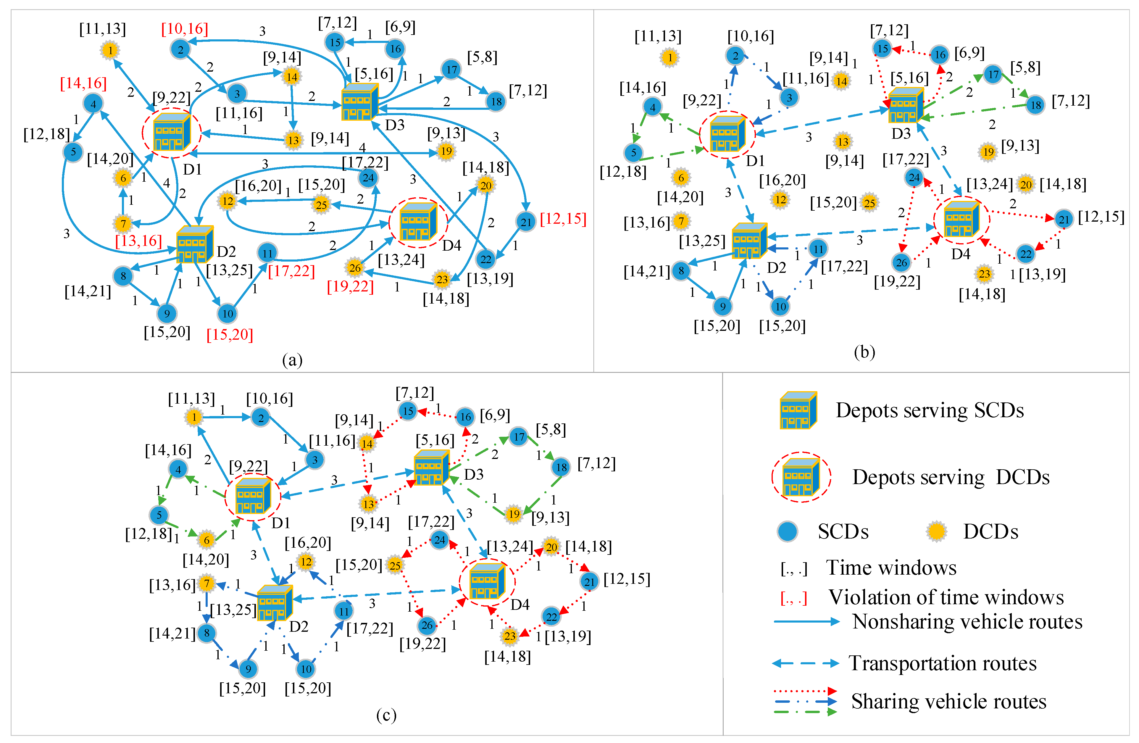
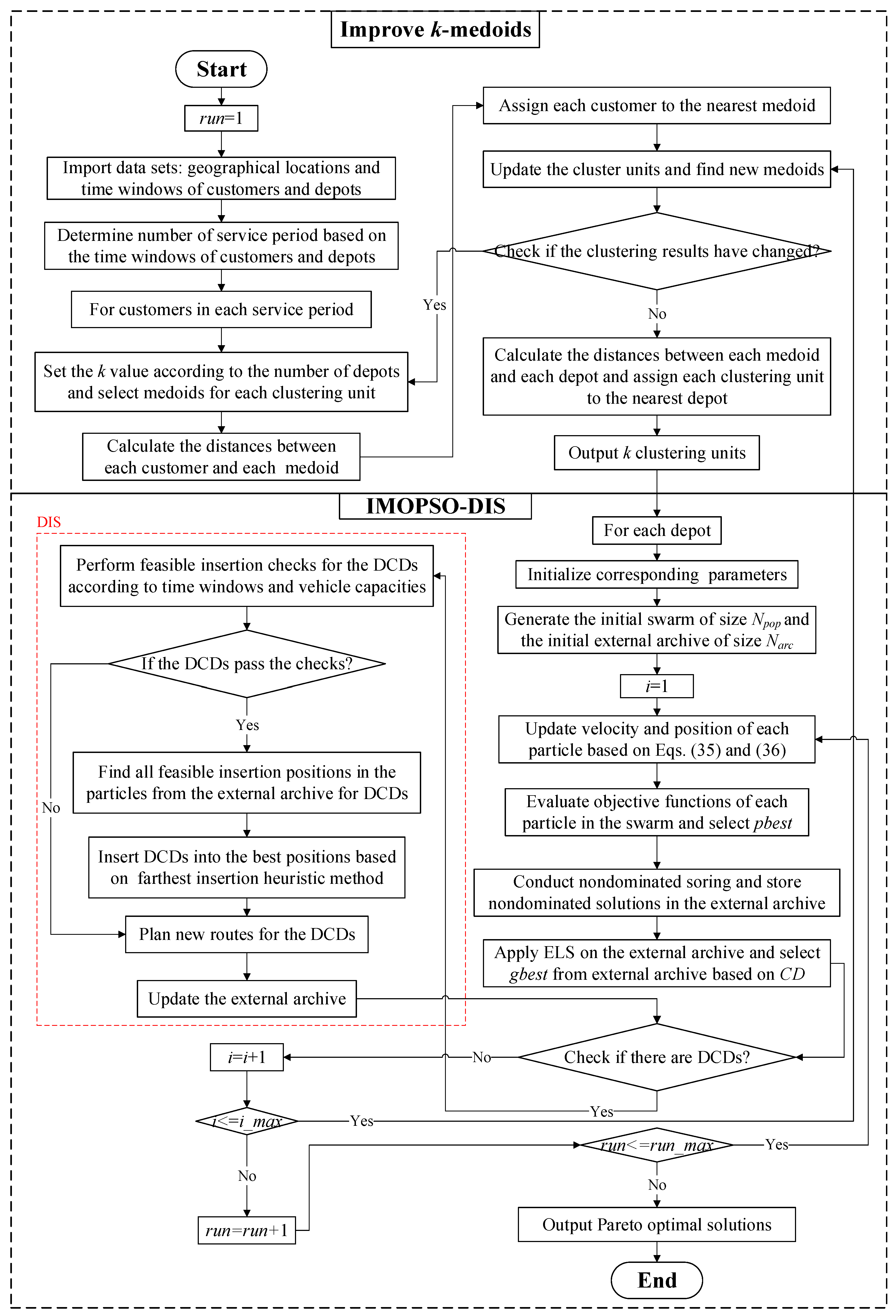
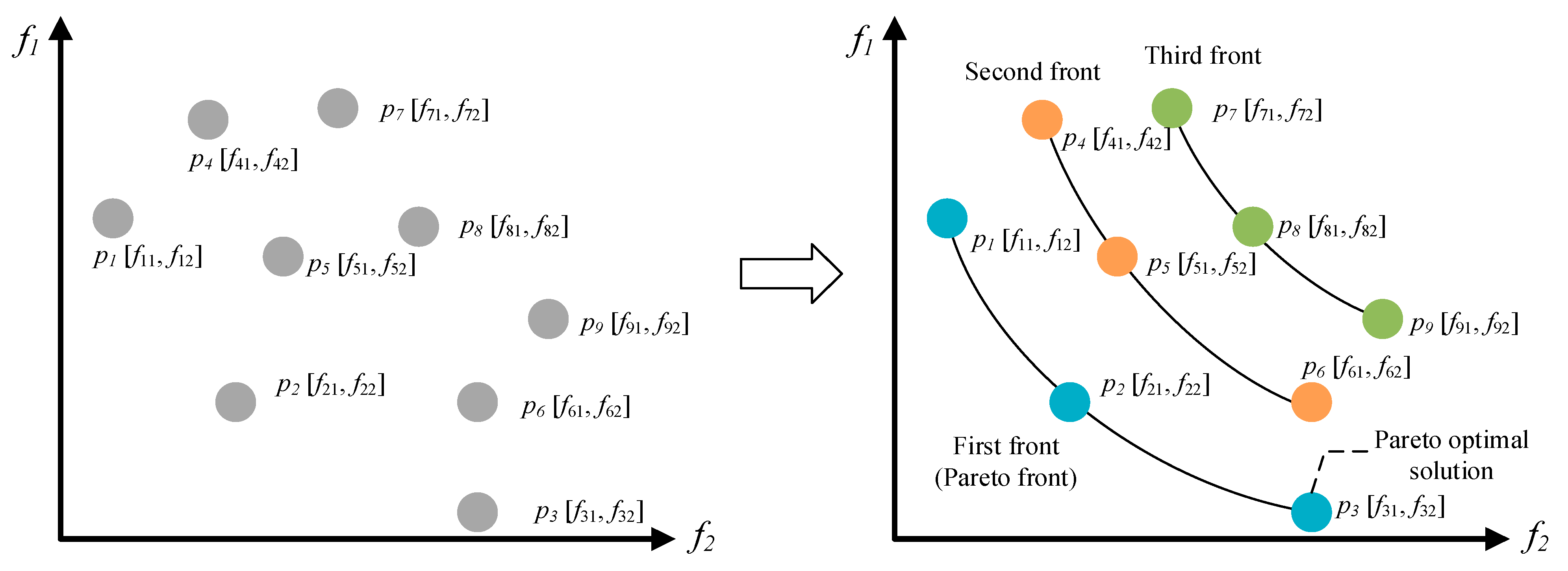
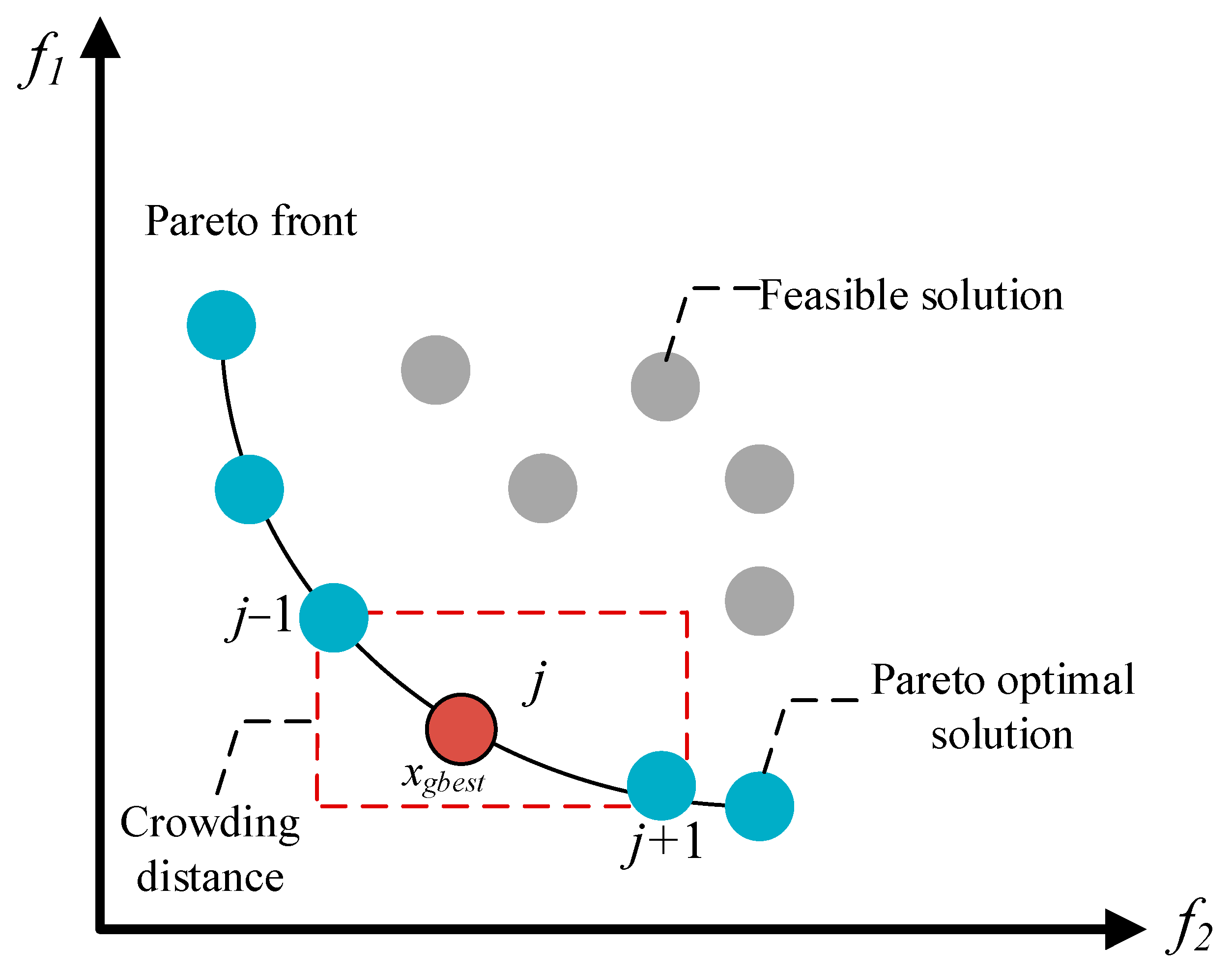

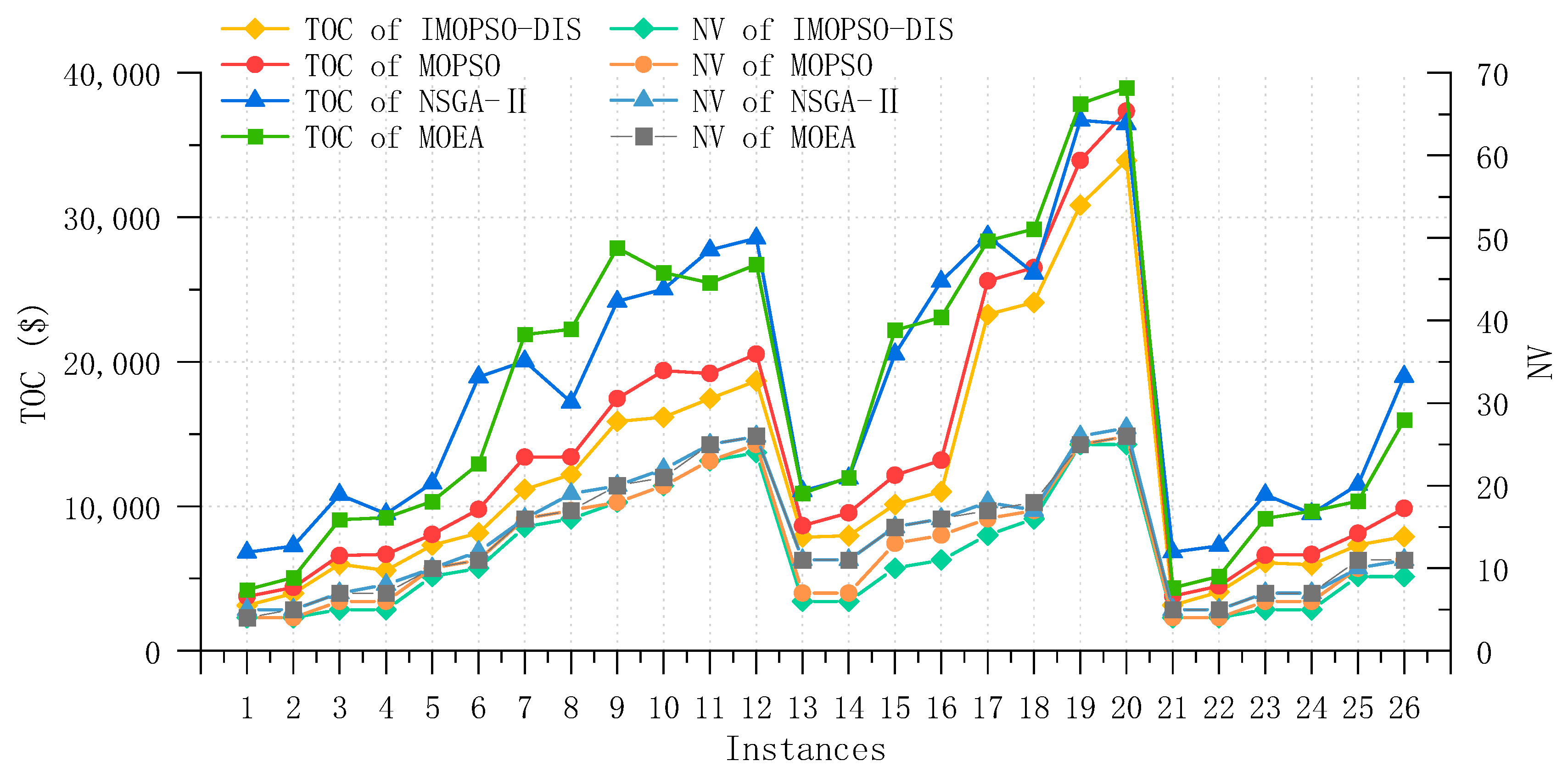
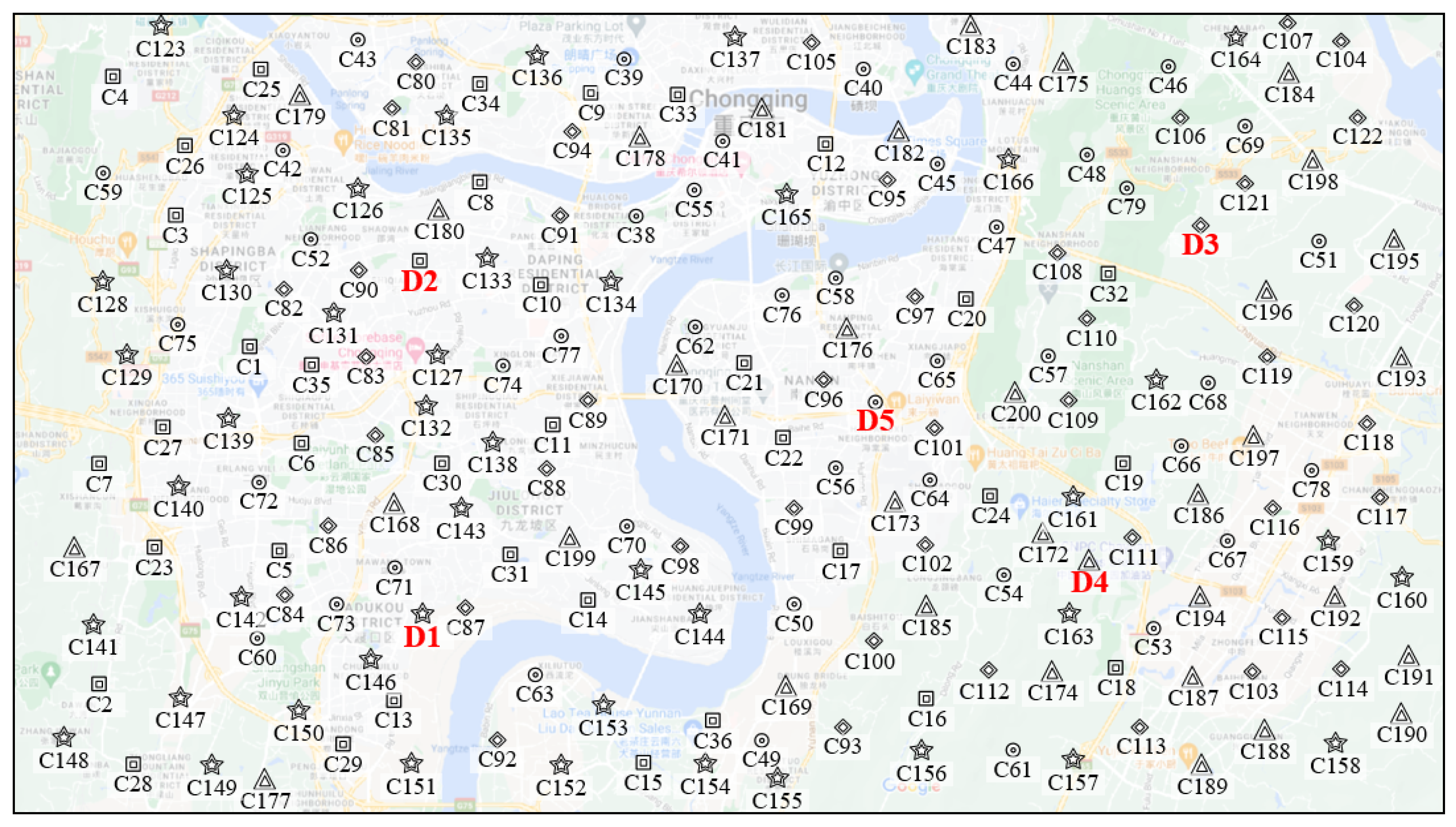
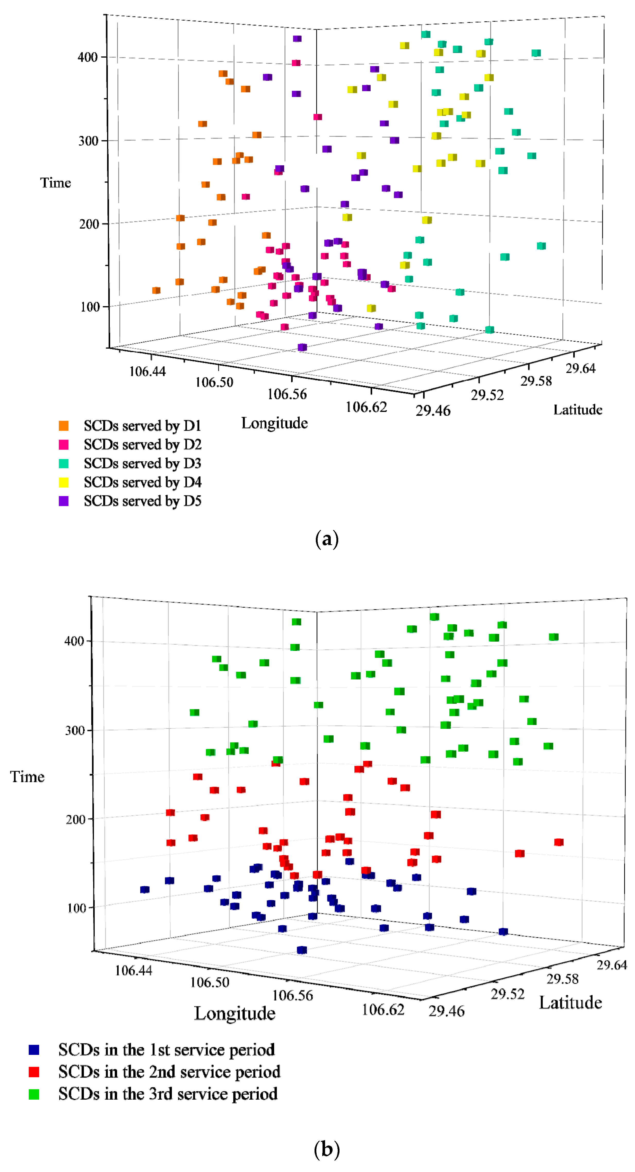
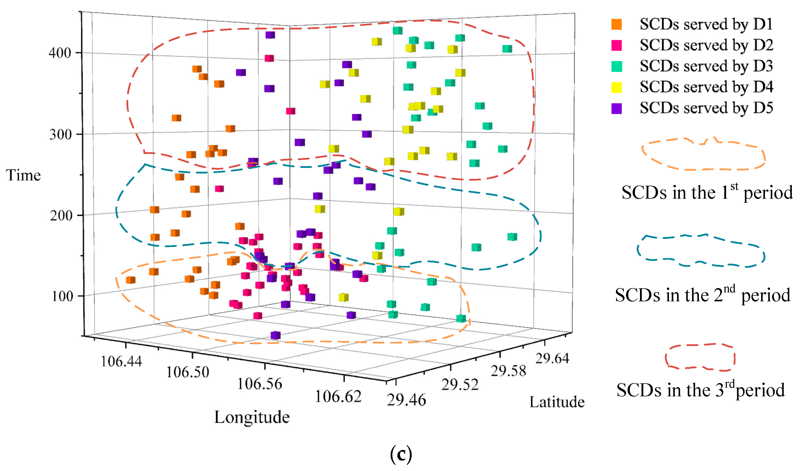
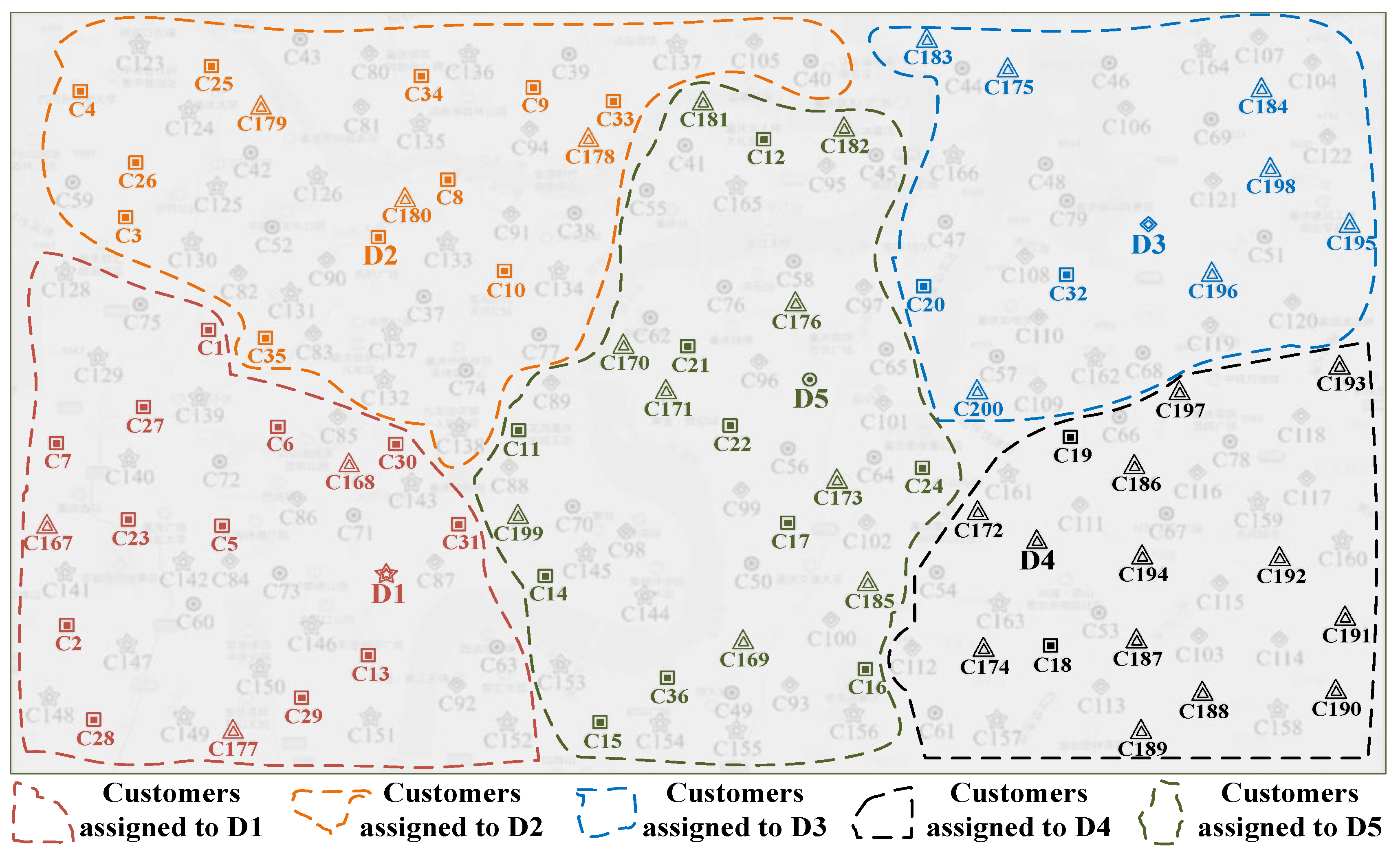
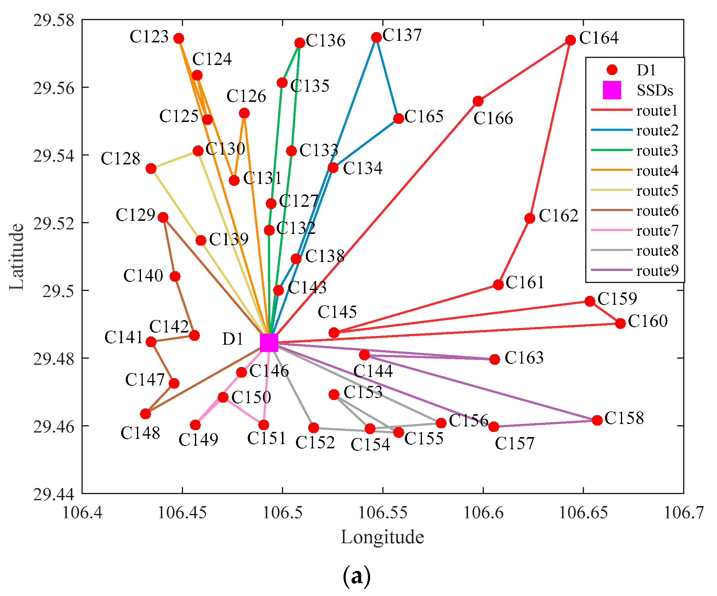
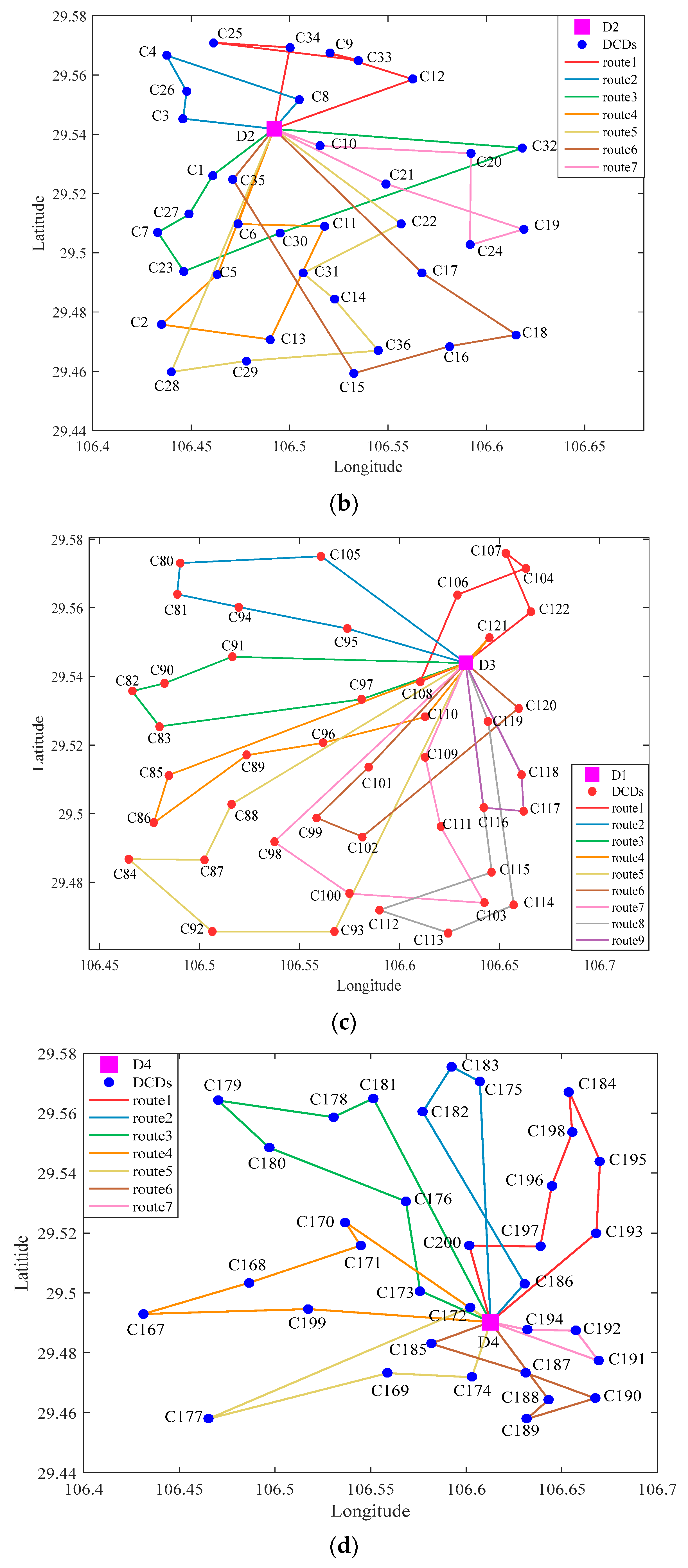
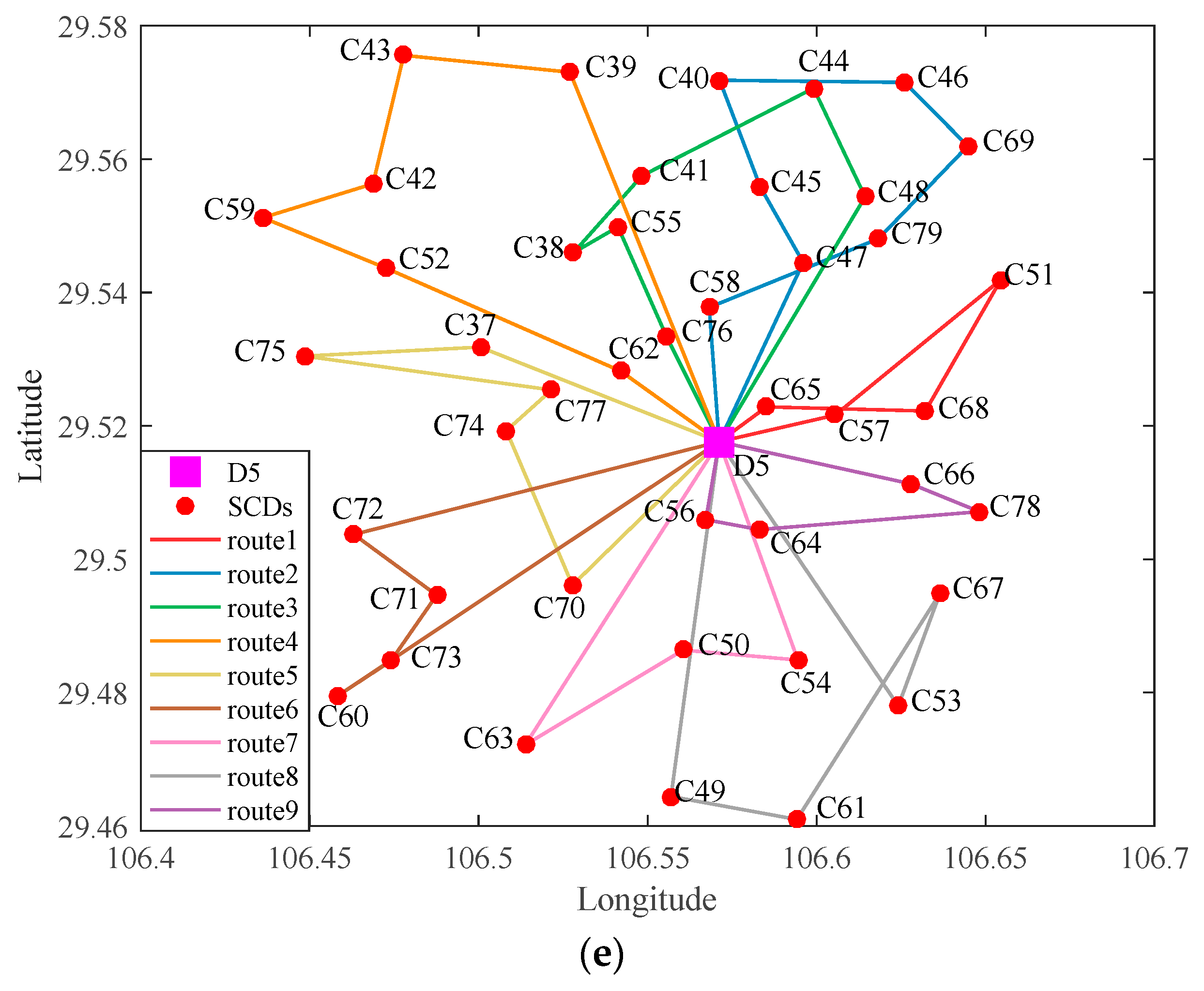
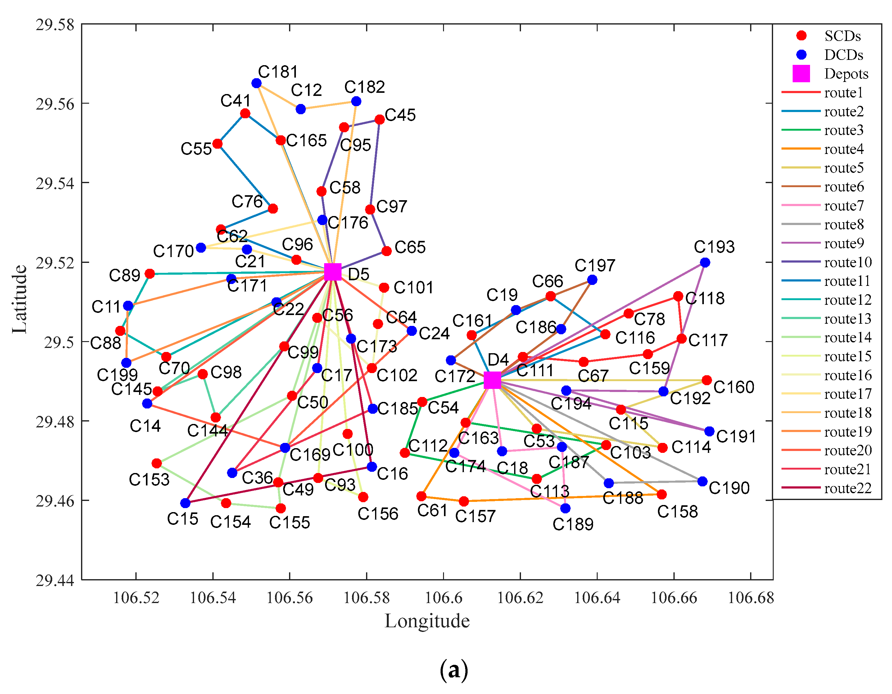
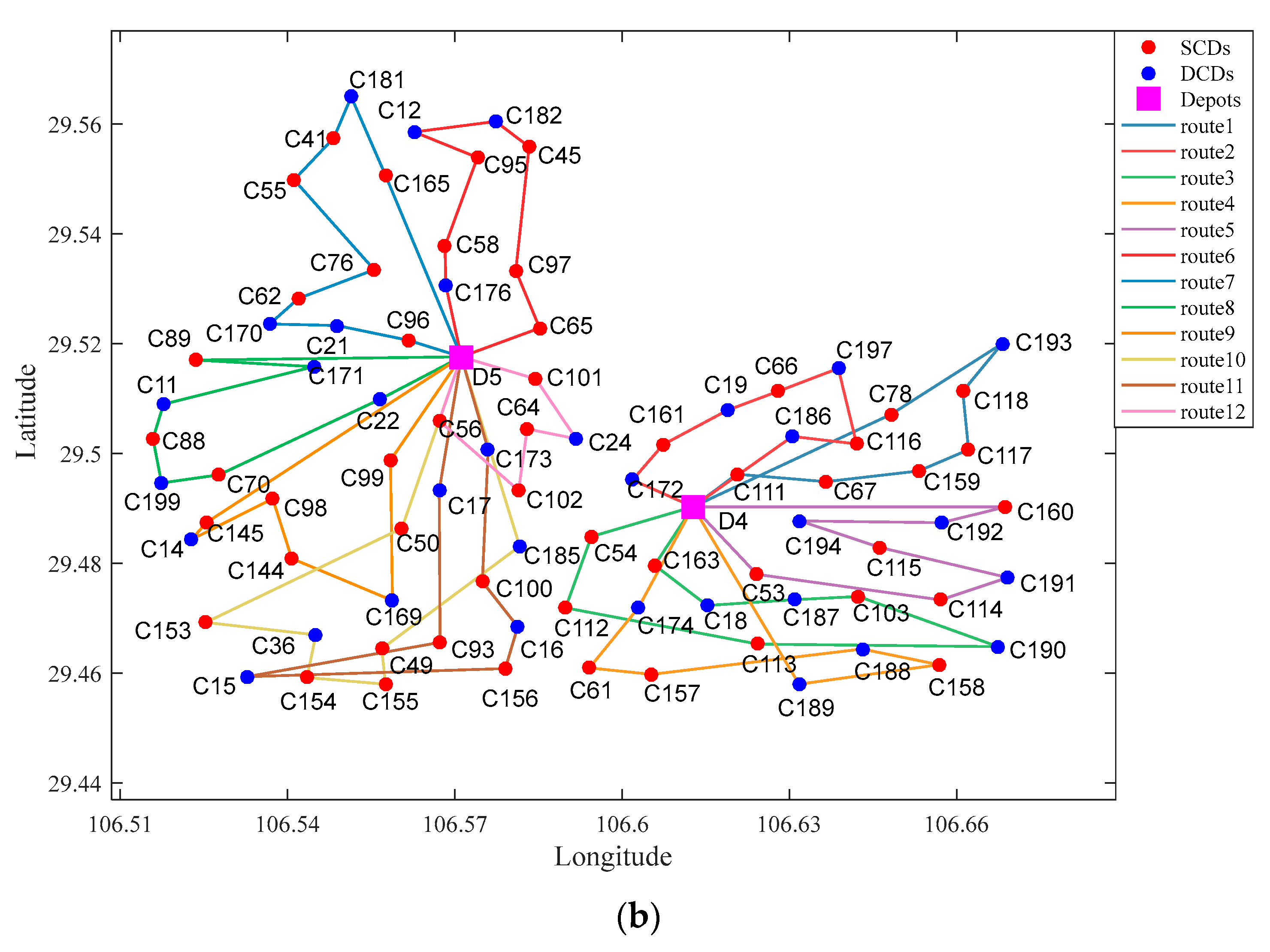
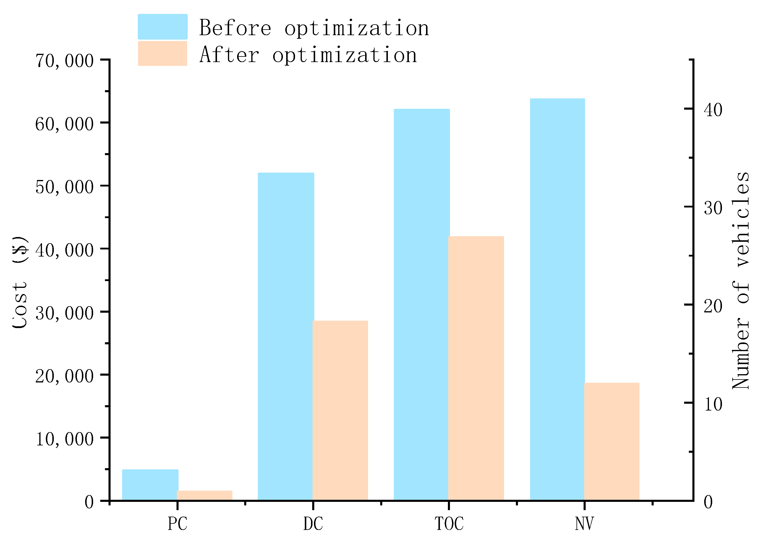
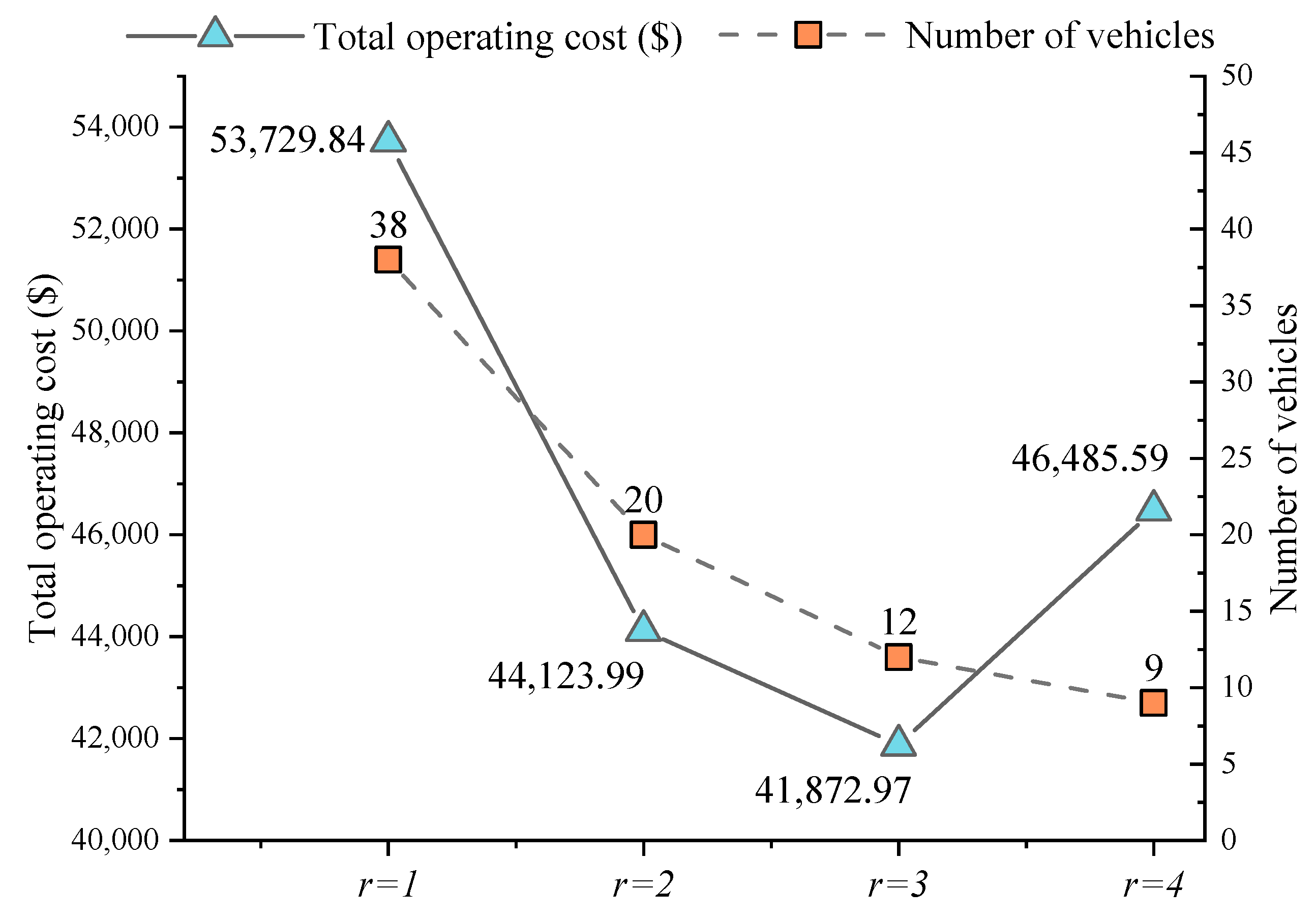
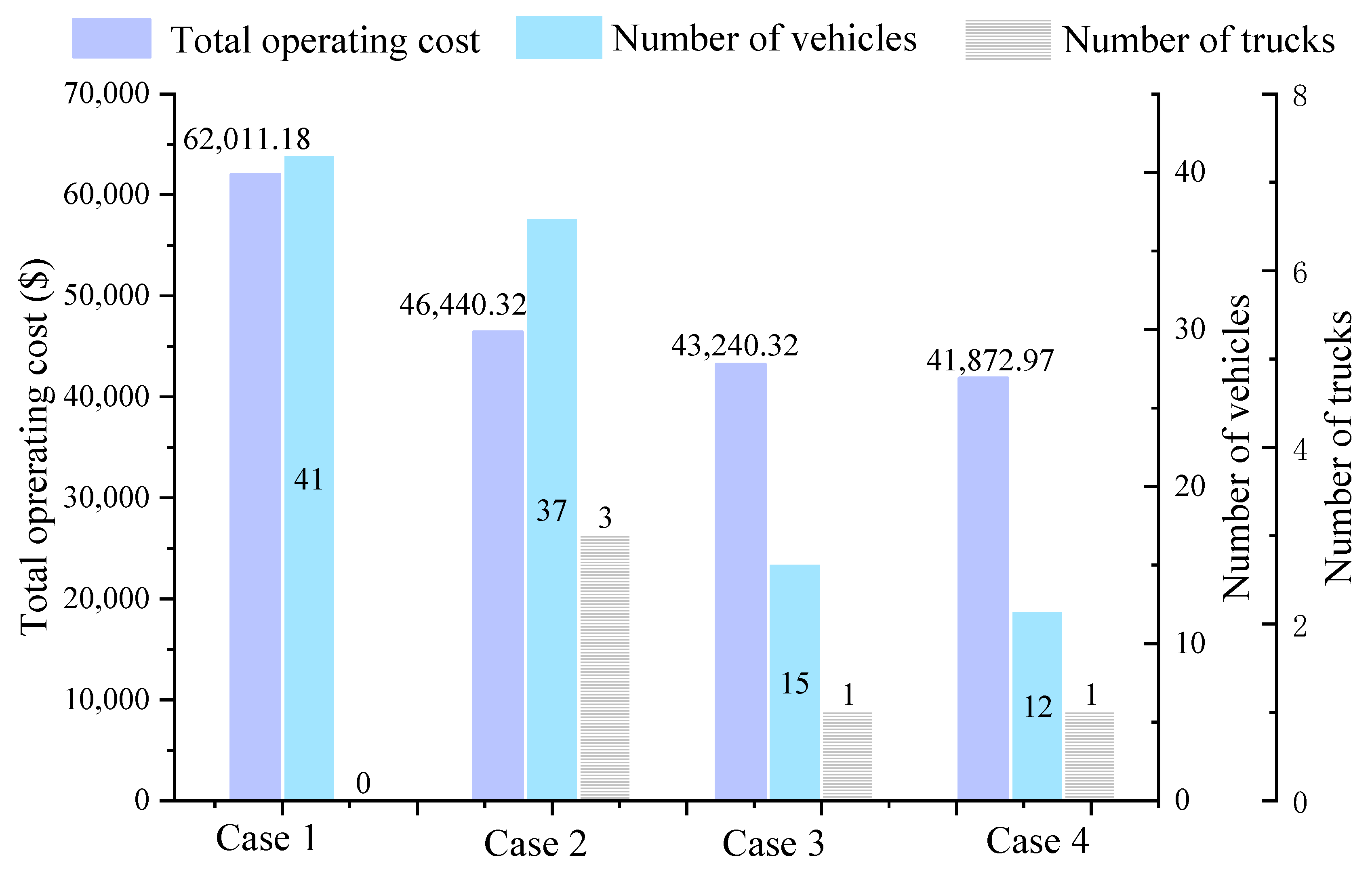


Publisher’s Note: MDPI stays neutral with regard to jurisdictional claims in published maps and institutional affiliations. |
© 2022 by the authors. Licensee MDPI, Basel, Switzerland. This article is an open access article distributed under the terms and conditions of the Creative Commons Attribution (CC BY) license (https://creativecommons.org/licenses/by/4.0/).