Electric Vehicle Charging Station Location-Routing Problem with Time Windows and Resource Sharing

Abstract

Electric vehicles (EVs) are widely applied in logistics companies’ urban logistics distribution, as fuel prices increase and environmental awareness grows. This study introduces an EV charging station (CS) location-routing problem with time windows and resource sharing (EVCS-LRPTWRS). Resource sharing, among multiple depots within multiple service periods is proposed to adjust the transportation resource configuration for a sustainable logistics development. Solving the EVCS-LRPTWRS involves a periodic CS location selection and a multi-depot multi-period EV routing optimization. A bi-objective nonlinear programming model is proposed to formulate the EVCS-LRPTWRS with a minimum total operating cost and number of EVs. A hybrid algorithm combining the Gaussian mixture clustering algorithm (GMCA) with the improved nondominated sorting genetic algorithm-II (INSGA-II) is designed to address the EVCS-LRPTWRS. The GMCA is employed to assign customers to appropriate depots in various service periods in order to reduce the computational complexity. The INSGA-II is adopted to obtain the Pareto optimal solutions by using the CS insertion operation to select CS locations and integrating the elite retention mechanism to ensure a stable and excellent performance. The superiority of the hybrid algorithm is proven by comparison with the other three algorithms (i.e., multi-objective genetic algorithm, multi-objective particle swarm optimization, and multi-objective ant colony optimization). An empirical study of the EVCS-LRPTWRS in Chongqing City, China is conducted. Then, four types of service period divisions and three scenarios of resource sharing modes are further analyzed and discussed. The empirical results demonstrate the validity and practicability of the proposed solution method in realizing a sustainable operation in EV distribution networks.

1. Introduction

Company decision-makers have focused on the concepts of sustainable operations and green transportation due to the increasing concern about global warming and environmental pollution [1,2]. Electric vehicles (EVs) are low-carbon transportation devices that can reduce harmful emissions and dependence on fossil fuels. These EVs are also a promising tool for developing sustainable logistics distribution networks [2,3]. However, two main challenges exist in the implementation of EV distribution. On the one hand, the lack of charging infrastructure hinders the spread of the EV distribution [4]. On the other hand, the restriction of EVs caused by a limited driving range and necessary charging time, and the growing demand for goods distribution, promote the occurrence of an unreasonable EV scheduling [4,5,6]. Therefore, optimizing the EV charging station (CS) location routing problem (EVCS-LRP) by integrating the transportation resource sharing strategy and service periods division is crucial to improving the efficiency of the EV distribution networks.

EV routing planning depends on the availability of CSs, and the selection of CS locations will be determined according to the delivery routes. This notion means that integrating EV scheduling into CS locations is essential [7,8]. The optimization of the locations of CSs and EV routes reduces the construction cost of EV distribution networks [9]. Furthermore, a transportation resource sharing strategy, as an effective method to optimize logistics operations in the urban freight industry, can reduce the number of required EVs, thus decreasing the environmental impact and avoiding traffic congestion [10,11]. Meanwhile, the division of multiple service periods in the whole planning horizon to further facilitate resource sharing among multiple depots, contributes to the rationalization of resource allocation and improvement of the efficiency and sustainability of the EV distribution networks [12,13].

The EV CS location-routing problem with time windows and resource sharing (EVCS-LRPTWRS) is presented and solved in this study. The CS location decisions and EV routing schemes are optimized among multiple depots within various service periods, and the transportation resource sharing strategy is applied to rationalize the resource configuration. A bi-objective nonlinear mathematical programming model with multiple service periods is formulated to minimize the total operating cost (TOC) and the number of required EVs. A hybrid algorithm composed of the Gaussian mixture clustering algorithm (GMCA) and an improved nondominated sorting genetic algorithm-II (INSGA-II) is proposed to address the EVCS-LRPTWRS. To simplify the logistics network optimization, customers are assigned to appropriate depots and divided into suitable service periods according to the GMCA. Then, the Pareto optimal solutions, including the optimal delivery routes and the CS location decisions are obtained by integrating the CS insertion operation into the NSGA-II. The application of the EVCS-LRPTWRS is verified by an empirical study. The results show that the proposed nonlinear programming model and hybrid algorithm can effectively optimize the CS location-routing problem and improve the EV delivery efficiency.

The contributions of this study are as follows: (1) A multi-depot multi-period EV distribution network is presented according to the periodic characteristics of the depots and customers, to determine the CS locations and optimize the EV delivery routes. (2) A transportation resource sharing strategy is integrated into the EVCS-LRPTWRS to improve the transportation efficiency and optimize resource configuration among multiple depots within various service periods. (3) A bi-objective nonlinear programming model integrating multiple service periods, a transportation resource sharing strategy, and a centralized transportation is constructed to minimize the operating cost and number of EVs. (4) A hybrid algorithm consisting of the GMCA and INSGA-II is developed to solve the bi-objective nonlinear programming model and obtain the Pareto optimal solutions including the CS location decisions and EV routes.

The remainder of this study is organized as follows. The related literature is described in Section 2. The problem of the EVCS-LRPTWRS is presented in Section 3. The related definitions and model formulation are elaborated in Section 4. The hybrid algorithm is developed in Section 5. The computational experiments are illustrated in Section 6. The conclusion and future research directions of this study are summarized in Section 7.

2. Literature Review

Recently, an increasing number of academic experts and enterprisers have started to pay attention to EVCS-LRP research due to the growing environmental awareness [14,15]. Moreover, EVCS-LRP-related research has grown in complexity. For example, common constraints such as multi-depot, time windows, and multi-period, are added to the standard EV location routing problem (EVLRP) to form various variants [16,17]. Meanwhile, transportation resource sharing is studied by an increasing number of researchers as a promising strategy to reduce the economic and environmental impacts of traffic congestion [10,11]. Researchers have developed a variety of related methods to address the complex problem [17,18].

2.1. Electric Vehicle Charging Station Location-Routing Problem

EVCS-LRP refers to simultaneously solving the CS location selection and EV routing optimization problems [7,19,20]. Yang and Sun [21] formulated an integer programming model to simultaneously decide the locations of battery swap stations (BSSs) and the route plan of EVs. Yıldız et al. [22] developed an enhanced deviation flow refueling location model to handle the refueling location station problem with routing by setting a tolerable shortest routing deviation. Schiffer and Walther [7] discussed the impact of different objective functions, such as the distance, the number of EVs and the required CSs, and the cost minimization, on the EV routing plan and CS location decisions. He et al. [23] proposed a bi-level programming model to determine the CS locations by maximizing the routing flow and balancing the routing plan under the constraint of the driving distance. Zhang et al. [24] introduced two resource strategies based on battery and loading capacities to determine the optimal number and locations of BSSs and the routes for the BSS location-routing problem. Guo et al. [25] developed a mathematical planning model based on user satisfaction and the detour limitations to solve the selection of service station locations and route planning for EVs. Çalık et al. [26] constructed a mixed integer programming model to minimize the total cost, including the routing costs and operating costs of CSs and EVs, in determining the location of CSs and the routes for EVs. Yang et al. [1] presented an optimization model based on a space time state energy representation network in the EVCS-LRP to reduce the operating cost and improve efficiency.

2.2. Electric Vehicle Location-Routing Problem and its Variants

The EVLRP and its variants, such as multi-depot, time windows, and multi-period, have been extensively studied in recent years [16,17]. Wang et al. [27] studied a multi-depot EV scheduling problem to minimize the total costs, including the fixed costs, travel costs and charging costs (CC) of EVs. Sadati and Çataya [28] defined a mixed integer linear programming model to address a multi-depot green vehicle routing problem (MDGVRP). The location-routing problem with time windows has been studied due to the significant influence of time windows on evaluating the efficiency of EV distribution networks [29,30]. Ghobadi et al. [2] translated the time constraints into cost in terms of economy and customer satisfaction to penalize the time window violations in the multi-depot EV routing problem (EVRP). Lam et al. [29] established an electric vehicle problem with time windows and considered the limitations of the CS capacities and the piecewise-linearity of charging times. Furthermore, a multi-period location routing problem was studied to satisfy the different time requirements of customers [12,13]. Li et al. [31] established a multi-period, multi-route CS location model to obtain the cost-effective location scheme from the spatial and temporal dimensions. Neves-Moreira et al. [32] proposed a novel mathematical formulation to deal with the multi-period vehicle routing problem with refueling decisions. Lin et al. [33] explored the impact of different service periods on the optimization results for the multi-period EV routing optimization problem.

2.3. Transportation Resource Sharing Strategy

Transportation resource sharing, which is an effective strategy to save logistics resources and costs where improving the efficiency of logistics networks, is conducive to the sustainable development of logistics [13,34]. Brandstätter et al. [34] combined the respective strengths of car sharing and EVs to overcome the challenges of traffic congestion and environmental pollution. Friedrich and Noekel [35] discussed the advantages of vehicle sharing systems in public transport networks and provided an assignment model for solving a vehicle sharing problem. Wang et al. [13] incorporated the transportation resource sharing strategy into the MDGVRP to eliminate long empty trips and improve the flexibility of the network and the efficiency of resource management. Almouhanna et al. [36] allowed all EVs to be shared among the depots in the electric location routing problem to save resources. Jin et al. [37] proposed a sharing mode of EVs and studied the various pricing strategies to improve the utilization rate of shared vehicles. Wang et al. [12] demonstrated that transportation resource sharing among multiple service periods can maximize resource utilization.

2.4. Relevant Solution Methods for Electric Vehicle Location-Routing Problem

Researchers consider the EVLRP to be a NP-hard problem that is primarily addressed via heuristic algorithms [18,38], machine learning [39,40], and evaluation methods [41,42]. Chen et al. [38] developed a heuristic branch-and-price algorithm with an adaptive selection scheme to simultaneously determine the locations of BSSs and the routing plan. Barco et al. [43] presented a differential evolution algorithm to coordinate the EV routing and recharge scheduling for solving the EVRP. Kyriakakis et al. [44] proposed an ant colony optimization algorithm as a solution method for the EVRP to minimize the energy consumption of EVs. Zhang et al. [45] incorporated a Gaussian variation operator, a differential evolution operator, and a congestion factor into the whale optimization algorithm to solve the CS location problem of EVs. Yu et al. [46] developed an adaptive larger neighborhood search (ALNS) algorithm to improve performance by specific removal and insertion operations of CSs in solving the variant of the EVRP with a mixed fleet. Erdem [47] designed an adaptive variable neighborhood search (AVNS) to optimize the routing with heterogeneous EVs for a sustainable urban recycling waste collection.

Table 1. Abbreviations of the relevant literature for the EVCS-LRPTWRS.

Abbreviation	Type of Problem	Abbreviation	Solution Method
EVLRPTW	Electric vehicle location-routing problem with time windows	VNS	Variable neighborhood search
MDEVLRPTW	Multi-depot electric vehicle location routing problem with time windows	MOPSO	Multi-objective particle swarm optimization
EVLRP-BSS	Electric vehicle location-routing problem with a battery swap station	LNS	Large neighborhood search
E2EVRP	Two-level electric vehicle routing problem	MOHA	Multi-objective heuristic algorithm
GVRP-PR	Green vehicle routing problem with partial charging	CG	Column generation
EVRP-BSS	Electric vehicle routing problem with a battery swap station	BP	Biased-randomized
EVRPTW	Electric vehicle routing problem with time windows	PSO	Particle swarm optimization

lists the abbreviations of the relevant literature for the EVCS-LRPTWRS and

Table 2. Relevant literature overview for the EVCS-LRPTWRS.

References	Type of Problems	Variants				Electric Fleet		Resource Sharing	Solution Method
		Multi-Depot	Multi-Echelon	Time Windows	Multi-Period	Homogeneous	Heterogeneous
Yang et al. [1]	EVLRP			√			√		Lagrange relaxation
Schiffer and Walther [7]	EVLRPTW			√		√			VNS
Wang et al. [12]	MDGVRP	√	√	√			√	√	MOPSO
Paz et al. [20]	MDEVLRPTW	√		√		√			CPLEX
Yang and Sun [21]	EVLRP-BSS					√			ALNS
Zhang et al. [24]	EVLRP-BSS					√			Hybrid VNS-PSO
Guo et al. [25]	EVLRP			√		√			K-shortest ALNS
Çalık et al. [26]	EVLRP			√			√		Integer programming
Brandstätter et al. [34]	CS location problem							√	Heuristic algorithm
Almouhanna et al. [36]	EVLRP	√				√		√	BR-VNS
Breunig et al. [48]	E2EVRP		√			√			LNS
Chakraborty et al. [49]	EVRP					√			MOHA
Felipe et al. [50]	GVRP-PR						√		VNS
Froger et al. [51]	EVRP			√			√		Labeling algorithm
Jie et al. [52]	EVRP-BSS		√			√			CG-ALNS
Hof et al. [53]	EVLRP-BSS			√		√			AVNS
Ma et al. [54]	EVRP			√		√		√	ALNS
Pelletier et al. [55]	EVRP			√		√			LNS
Zhu et al. [56]	CS location problem			√					Genetic algorithm
Keskin and Çatay [57]	EVRPTW	√		√			√		ALNS
This work	EVCS-LRPTW	√	√	√	√		√	√	INSGA-II

summarizes the relevant studies for the EVCS-LRPTWRS.

In Table 2, a comparison of 20 previous papers with the proposed study was presented. The comparison content is divided into the following five aspects: (1) type of problems; (2) variants of the multi-depot, multi-echelon, time windows, and multi-period; (3) type of electric fleet: homogeneous or heterogeneous; (4) resource sharing strategy; and (5) solution method. According to the comparison results, the aspects considered in this study are comprehensive.

The limitations of the aforementioned literature for the EVCS-LRPTWRS optimization are as follows: (1) CS location decisions and EV routes in the multi-depot multi-period logistics network design have insufficiently been discussed. (2) The transportation resource sharing strategy is rarely considered in the optimization of the EVCS-LRP. (3) An effective mathematical model for a resource sharing strategy and centralized transportation in the optimization of the EVCS-LRPTWRS is lacking. (4) Existing heuristic algorithms have limited applicability in solving the EVCS-LRPTWRS within multiple service periods considering a shared transportation resource.

3. Problem Statement

The optimization of the EVCS-LRPTWRS is advantageous in designing an efficient logistics network and reducing the environmental impact of the logistics operations [13,36,58]. The EVCS-LRPTWRS aims to simultaneously deal with the location selection of CSs and the routing optimization in the multi-depot multi-period EV distribution network. The EV distribution network consists of multiple depots, several candidate CSs, and a number of customers. Multiple depots are connected by electric trucks (ETs), and customers are served by EVs from depots. The number and location of CSs should be determined and selected from the candidate CSs to satisfy the charging needs of EVs during the delivery process. In addition, a working period can be divided into several service periods based on the different time windows of depots and customers. Specifically, each depot has several operating time windows, and every customer has a service time window during a work period. Figure 1 illustrates the comparison of the EVCS-LRPTWRS before and after optimization.

Figure 1a shows the initial EV distribution network before optimization. In this study, EVs need a significant amount of power on the way to serve customers due to the inappropriate use of the CSs, resulting in a large portion of electricity consumption (EC) and waste of transportation resources. Moreover, the irrational resource configuration inevitably leads to the occurrence of long-distance and crisscross transportation, thus making considerable violations of customers’ time windows. The independence of the delivery routes between two service periods of depots causes a large number of required EVs. Figure 1b shows the optimized CS location-routing network. A more orderly EV distribution network without long-haul and overlapping delivery routes is organized by the optimized location selection of CSs. The sets of CSs selected to provide charging services for EVs in the two service periods are {CS2, CS4} and {CS4, CS6}, and the location selections of CSs are independent between the two service periods. In comparison with the initial EV distribution network, an ET can transport goods to multiple depots while meeting the time windows of all depots, and the number of customers served beyond the required time windows has been significantly reduced. In addition, each EV can cover several routes to cover the share of transportation resources among the various service periods. For example, routes D3→C17→C16→CS4→C15→D3 and D3→C18→C19→D3 are visited by EV3 within the first service period, and EV3 continues to implement route D2→C12→C13→CS6→C11→D2 within the second service period. Therefore, the optimization of the CS location-routing network and transportation resource sharing strategy is effective in improving the utilization of transportation resources and achieving EC savings.

We assume that the EC of EVs is only related to unit time, and 8 kWh per unit time for EC, USD 3 per kWh for electricity prices, USD 15 per time unit for penalty cost (PCs) (earliness and delay penalties), USD 5 per time unit for CC, and USD 25 per time unit for centralized transportation cost (CTC).

Table 3. Comparison in the initial and optimized network of the EVCS-LRPTWRS.

Case	Service Period	CTC (USD)	EDC (USD)	EC (kWh)	CC (USD)	Waiting and Delay Times	PC (USD)	TOC (USD)	Number of EVs	Number of ETs	Selected CSs
Initial	1st	0	672	224	100	18	270	1042	6	0	4
	2nd	0	672	224	70	4	60	802	5	0	2
	Total	0	1344	448	170	22	330	1844	11	0	6
Optimized	1st	225	456	152	70	1	15	766	3	1	2
	2nd	0	384	128	60	0	0	444	3	0	2
	Total	225	840	280	130	1	15	1210	3	1	3

compares ten indicators related to the optimization of the EVCS-LRPTWRS, including the CTC, electric delivery cost (EDC), EC, PC, CC, TOC, number of EVs, number of ETs, and number of selected CSs.

In Table 3, the total cost and number of EVs were reduced by designing a CS location-routing network. The TOC decreases from USD 1844 to USD 1210 for the two service periods through the optimization of the EVCS-LRPTWRS, achieving a total saving of USD 634. The number of EVs decreases from 11 to 3, with a drop of 8. The number of selected CSs decreases from 6 to 3, with a reduction of 3. Furthermore, the EC decreases from 448 kWh to 280 kWh, with an electricity-saving of 168 kWh. Therefore, the EVCS-LRPTWRS optimization can effectively reduce the operating cost and improve the utilization of the transportation resource for the EV distribution network.

4. Related Definitions and Model Formulation

4.1. Assumptions and Definitions

In this section, we develop a bi-objective nonlinear programming model to solve the charging infrastructure location problem integrated with the planning of the EV distribution routing problem. To clarify the EVCS-LRPTWRS model, the relevant notations and variables used in the model are defined in

Table 4. Notations and descriptions used in the EVCS-LRPTW model.

Sets	Definitions
D	Set of depots, D = {1, 2, 3, …, d}, d∈D
C	Set of customers, C = {1, 2, 3, …, c}, c∈C
R	Set of CSs, R = {1, 2, 3, …, r}, r∈R
T	Set of electric trucks for centralized transportation, T = {1, 2, 3, …, t}, t∈T
V	Set of EVs for delivery routes, V = {1, 2, 3, …, v}, v∈V
W	Set of service periods within one working period, W = {1, 2, 3, …,w}, w∈W
$M_t^w$	$\mathrm{The} \mathrm{sequence} \mathrm{of} \mathrm{routes} \mathrm{executed} \mathrm{by} \mathrm{ET} t \mathrm{within} \mathrm{the} w\mathrm{th} \mathrm{service} \mathrm{period}, M_t^w$$=\{1, 2, 3, \dots , m\}, m\in M_t^w$, t∈T, w∈W
$N_v^w$	$\mathrm{The} \mathrm{sequence} \mathrm{of} \mathrm{routes} \mathrm{executed} \mathrm{by} \mathrm{EV} v \mathrm{within} \mathrm{the} w\mathrm{th} \mathrm{service} \mathrm{period}, N_v^w$$=\{1, 2, 3, \dots , n\}, n\in N_v^w$, v∈V, w∈W
$U_v^w$	Set of EVs used to serve customers within the wth service period, v∈V, w∈W
$N{U}_{vn}^w$	$\mathrm{Set} \mathrm{of} \mathrm{customers} \mathrm{served} \mathrm{by} \mathrm{EV} v \mathrm{in} \mathrm{the} \mathrm{nth} \mathrm{route} \mathrm{within} \mathrm{the} w\mathrm{th} \mathrm{service} \mathrm{period}, n\in N{U}_{vn}^w$, v∈V, w∈W
Parameters	Description
fe	Electricity price, (unit: USD/kWh)
Fcc	CC of electricity per unit time, (unit: USD/h)
FRr	Unit operating cost of CS
${\delta }_v$	Charging rate of EV v, v∈V, (unit: kWh/h)
${\mu }_d$	Variable cost coefficient of depot d, d∈D
MNv	Annual maintenance cost of EV v, v∈V
K	Number of working periods in one year
$EC{V}_{dcvn}^w$	$\mathrm{EC} \mathrm{of} \mathrm{EV} v \mathrm{from} \mathrm{node} d \mathrm{to} c \mathrm{in} \mathrm{the} n\mathrm{th} \mathrm{route} \mathrm{within} \mathrm{the} w\mathrm{th} \mathrm{service} \mathrm{period}, d, c\in R\cup D\cup C, d\ne c, v\in V, n\in N_v^w$, w∈W, (unit: kWh)
$EC{T}_{dd\prime tm}^w$	$\mathrm{EC} \mathrm{of} \mathrm{ET} t\mathrm{from} \mathrm{depot} d \mathrm{to} d’ \mathrm{in} \mathrm{the} m\mathrm{th} \mathrm{route} \mathrm{within} \mathrm{the} w\mathrm{th} \mathrm{service} \mathrm{period}, d, d’\in D, d\ne d’, v\in V, m\in M_t^w$, w∈W,(unit: kWh)
αv	Arc specific coefficient of EV v, v∈V
${\lambda }_t$	Arc specific coefficient of ET t, t∈T
${\gamma }_t$	Vehicle specific coefficient of ET t, t∈T
βv	Vehicle specific coefficient of EV v, v∈V
$S{V}_{dn}^w$	$\mathrm{Driving} \mathrm{speed} \mathrm{of} \mathrm{EV} v\mathrm{in} \mathrm{the} n\mathrm{th} \mathrm{route} \mathrm{within} \mathrm{the} w\mathrm{th} \mathrm{service} \mathrm{period}, v\in V, n\in N_v^w$, w∈W, (unit: m/s)
$S{T}_{tm}^w$	$\mathrm{Driving} \mathrm{speed} \mathrm{of} \mathrm{ET} t\mathrm{in} \mathrm{the} m\mathrm{th} \mathrm{route} \mathrm{within} \mathrm{the} w\mathrm{th} \mathrm{service} \mathrm{period}, t\in T, m\in M_t^w$, w∈W, (unit: m/s)
$WE{V}_{vn}^w$	$\mathrm{Weight} \mathrm{of} \mathrm{EV} v \mathrm{in} \mathrm{the} n\mathrm{th} \mathrm{route} \mathrm{within} \mathrm{the} w\mathrm{th} \mathrm{service} \mathrm{period}, v\in V, n\in N_v^w$, w∈W, (unit: kg)
$WE{T}_{tm}^w$	$\mathrm{Weight} \mathrm{of} \mathrm{ET} t \mathrm{in} \mathrm{the} m\mathrm{th} \mathrm{route} \mathrm{within} \mathrm{the} w\mathrm{th} \mathrm{service} \mathrm{period}, t\in T, m\in M_t^w$, w∈W, (unit: kg)
ldc	Distance from node d to c, d, c∈R∪D∪C, d ≠ c
Ldd’	Distance from depot d to d’, d, d’∈D, d ≠ d’
QTt	Load capacity of ET t, t∈T
QVv	Load capacity of EV v, v∈V
${\partial }_c^w$	Demand quantity of customer c within the wth service period, c∈C, w∈W
$q_{dd\prime }^w$	Transport quantity from depot d to d’ within the wth service period, d, d’∈D, d ≠ d’, w∈W
$q_d$	Demand quantity of depot d, d∈D
Pe	PC per unit of time of earliness
Pl	PC per unit of time of delay
$[e_d^w,l_d^w]$	Operation time window for depot d within the wth service period, d∈D, w∈W
$[g_c^w,h_c^w]$	Service time window for customer c within the wth service period, c∈C, w∈W
$L{T}_{dvn}^w$	$\mathrm{Departure} \mathrm{time} \mathrm{of} \mathrm{EV} v \mathrm{from} \mathrm{depot} d \mathrm{in} \mathrm{the} \mathrm{nth} \mathrm{route} \mathrm{within} \mathrm{the} w\mathrm{th} \mathrm{service} \mathrm{period}, d\in D, v\in V, n\in N_v^w$, v∈V, w∈W
$D{T}_{dtm}^w$	$\mathrm{Departure} \mathrm{time} \mathrm{of} \mathrm{ET} \mathrm{t} \mathrm{from} \mathrm{depot} \mathrm{d} \mathrm{in} \mathrm{the} m\mathrm{th} \mathrm{route} \mathrm{within} \mathrm{the} w\mathrm{th} \mathrm{service} \mathrm{period}, d\in D, t\in T, m\in M_t^w$, w∈W
$L{T}_{cvn}^w$	$\mathrm{Departure} \mathrm{time} \mathrm{of} \mathrm{EV} v \mathrm{from} \mathrm{customer} c \mathrm{in} \mathrm{the} n\mathrm{th} \mathrm{route} \mathrm{within} \mathrm{the} w\mathrm{th} \mathrm{service} \mathrm{period}, c\in C, v\in V, n\in N_v^w$,w∈W
$L{T}_{rvn}^w$	$\mathrm{Departure} \mathrm{time} \mathrm{of} \mathrm{EV} v \mathrm{from} \mathrm{CS} r \mathrm{in} \mathrm{the} n\mathrm{th} \mathrm{route} \mathrm{within} \mathrm{the} w\mathrm{th} \mathrm{service} \mathrm{period}, r\in R, v\in V, n\in N_v^w$, w∈W
$A{T}_{dvn}^w$	$\mathrm{Arrival} \mathrm{time} \mathrm{of} \mathrm{EV} v \mathrm{at} \mathrm{depot} d \mathrm{in} \mathrm{the} n\mathrm{th} \mathrm{route} \mathrm{within} \mathrm{the} w\mathrm{th} \mathrm{service} \mathrm{period}, d\in D, v\in V, n\in N_v^w$, w∈W
$G{T}_{dtm}^w$	$\mathrm{Arrival} \mathrm{time} \mathrm{of} \mathrm{ET} t \mathrm{at} \mathrm{depot} d \mathrm{in} \mathrm{the} n\mathrm{th} \mathrm{route} \mathrm{within} \mathrm{the} w\mathrm{th} \mathrm{service} \mathrm{period}, d\in D, t\in T, m\in M_t^w$, w∈W
$A{T}_{cvn}^w$	Arrival time of EV v at customer c in the nth route within the wth service period, c∈C, v∈V, n∈$N_v^w$, w∈W
$A{T}_{rvn}^w$	$\mathrm{Arrival} \mathrm{time} \mathrm{of} \mathrm{EV} v \mathrm{at} \mathrm{CS} r \mathrm{in} \mathrm{the} n\mathrm{th} \mathrm{route} \mathrm{within} \mathrm{the} w\mathrm{th} \mathrm{service} \mathrm{period}, r\in R, v\in V, n\in N_v^w$, w∈W
$W{T}_{cvn}^w$	$\mathrm{Waiting} \mathrm{time} \mathrm{of} \mathrm{EV} v \mathrm{at} \mathrm{customer} c \mathrm{in} \mathrm{the} n\mathrm{th} \mathrm{route} \mathrm{within} \mathrm{the} w\mathrm{th} \mathrm{service} \mathrm{period}, \mathrm{and} \mathrm{the} \mathrm{waiting} \mathrm{time} \mathrm{denotes} \mathrm{the} \mathrm{time} \mathrm{required} \mathrm{to} \mathrm{wait} \mathrm{for} \mathrm{the} \mathrm{service} \mathrm{to} \mathrm{start}, c\in C, v\in V, n\in N_v^w$, w∈W
$C{T}_{rvn}^w$	$\mathrm{Charging} \mathrm{time} \mathrm{of} \mathrm{EV} v \mathrm{at} \mathrm{CS} r \mathrm{in} \mathrm{the} n\mathrm{th} \mathrm{route} \mathrm{within} \mathrm{the} w\mathrm{th} \mathrm{service} \mathrm{period}, r\in R, v\in V, n\in N_v^w$, w∈W
$J{T}_{rcvn}^w$	$\mathrm{Travel} \mathrm{time} \mathrm{of} \mathrm{EV} v \mathrm{from} \mathrm{CS} r \mathrm{to} \mathrm{customer} c \mathrm{in} \mathrm{the} n\mathrm{th} \mathrm{route} \mathrm{within} \mathrm{the} w\mathrm{th} \mathrm{service} \mathrm{period}, r\in R, c\in C, v\in V, n\in N_v^w$,w∈W
$J{T}_{drvn}^w$	$\mathrm{Travel} \mathrm{time} \mathrm{of} \mathrm{EV} v \mathrm{from} \mathrm{customer} d \mathrm{to} \mathrm{CS} r \mathrm{in} \mathrm{the} n\mathrm{th} \mathrm{route} \mathrm{within} \mathrm{the} w\mathrm{th} \mathrm{service} \mathrm{period}$, r∈R, d∈C, v∈V,n∈$N_v^w$, w∈W
$J{T}_{dcvn}^w$	$\mathrm{Travel} \mathrm{time} \mathrm{of} \mathrm{EV} v \mathrm{from} \mathrm{customer} d \mathrm{to} c \mathrm{in} \mathrm{the} n\mathrm{th} \mathrm{route} \mathrm{within} \mathrm{the} w\mathrm{th} \mathrm{service} \mathrm{period}$, d, c∈C, d≠ c, v∈V, n∈$N_v^w$, w∈W
$L{E}_{rvn}^w$	Amount of electricity remaining when EV v leaves depot or CS r, r∈R∪D, v∈V, n∈$N_v^w$, w∈W, (unit: kWh)
$L{E}_{dvn}^w$	$\mathrm{Amount} \mathrm{of} \mathrm{electricity} \mathrm{remaining} \mathrm{when} \mathrm{EV} v \mathrm{leaves} \mathrm{customer} d, c\in C, v\in V, n\in N_v^w$, w∈W, (unit: kWh)
$L{E}_{cvn}^w$	Amount of electricity remaining when EV v leaves customer c, c∈C, v∈V, n∈$N_v^w$, w∈W, (unit: kWh)
$A{E}_{cvn}^w$	$\mathrm{Amount} \mathrm{of} \mathrm{electricity} \mathrm{remaining} \mathrm{when} \mathrm{EV} v \mathrm{arrives} \mathrm{at} \mathrm{customer} c, c\in C, v\in V, n\in N_v^w$, w∈W, (unit: kWh)
$R{E}_{rvn}^w$	$\mathrm{Amount} \mathrm{of} \mathrm{electricity} \mathrm{remaining} \mathrm{of} \mathrm{EV} v \mathrm{at} \mathrm{node} r, r\in R\cup D\cup C, v\in V, n\in N_v^w$, w∈W, (unit: kWh)
$C{E}_{drvn}^w$	$\mathrm{Amount} \mathrm{of} \mathrm{EC} \mathrm{of} \mathrm{EV} v \mathrm{from} \mathrm{customer} d \mathrm{to} \mathrm{CS} , c\in C, r\in R, v\in V, n\in N_v^w$, w∈W, (unit: kWh)
$C{E}_{rcvn}^w$	$\mathrm{Amount} \mathrm{of} \mathrm{EC} \mathrm{of} \mathrm{EV} v \mathrm{from} \mathrm{CS} \mathrm{to} \mathrm{customer} c, c\in C, r\in R, v\in V, n\in N_v^w$, w∈W, (unit: kWh)
$C{E}_{dcvn}^w$	$\mathrm{Amount} \mathrm{of} \mathrm{EC} \mathrm{of} \mathrm{EV} v \mathrm{from} \mathrm{customer} d\mathrm{to} c ,d,c\in C, d\ne c, v\in V, n\in N_v^w$, w∈W, (unit: kWh)
Ev	Battery capacity of EV v, v∈V, (unit: kWh)
MM	Extremely large number
$|N_v^w|$	Number of routes assigned to EV v within the wth service period
$|N{U}_{vn}^w|$	Number of customers served by EV v in the nth route within the wth service period
$|U_v^w|$	Number of EVs used to serve customers within the wth service period
Decision variable	Description
$x_{dcvn}^w$	$\mathrm{If} \mathrm{EV} v \mathrm{travels} \mathrm{from} \mathrm{node} d \mathrm{to} \mathrm{node} \mathrm{c} \mathrm{in} \mathrm{the} n\mathrm{th} \mathrm{route} \mathrm{within} \mathrm{the} w\mathrm{th} \mathrm{service} \mathrm{period} x_{dcvn}^w$$=1, \mathrm{otherwise}, x_{dcvn}^w$$=0, d, c\in R\cup D\cup C, d\ne c, v\in V, n\in N_v^w$, w∈W
${\pi }_{dd\prime tm}^w$	$\mathrm{If} \mathrm{ET} t \mathrm{travels} \mathrm{from} \mathrm{depot} d \mathrm{to} d’ \mathrm{in} \mathrm{the} m\mathrm{th} \mathrm{route} \mathrm{within} \mathrm{the} w\mathrm{th} \mathrm{service} \mathrm{period} {\pi }_{dd\prime tm}^w$$=1, \mathrm{otherwise}, {\pi }_{dd\prime tm}^w$$=0, d,d’\in D, d\ne d’, t\in T, m\in M_t^w$, w∈W
$x_{dcv}^w$	$\mathrm{If} \mathrm{EV} v \mathrm{travels} \mathrm{from} \mathrm{node} d \mathrm{to} \mathrm{node} c \mathrm{within} \mathrm{the} w\mathrm{th} \mathrm{service} \mathrm{period}, x_{dcv}^w$$=1; \mathrm{otherwise}, x_{dcv}^w$= 0, d, c∈R∪D∪C, d≠ c, v∈V, w∈W
${\phi }_v^w$	If EV v is selected to serve customers within the wth service period, v∈V, w∈W
$O_{dcd\prime }$	$\mathrm{If} \mathrm{customer} c \mathrm{is} \mathrm{reassigned} \mathrm{from} \mathrm{depot} d \mathrm{to} d’, O_{dcd\prime }$$=1; \mathrm{otherwise}, O_{dcd\prime }$= 0, d, d, d’∈D, d≠d’, c∈C, v∈V
$y_{rv}^{}$	$\mathrm{If} \mathrm{EV} v \mathrm{charged} \mathrm{at} \mathrm{CS} \mathrm{or} \mathrm{depot} r y_{rv}^{}$$=1; \mathrm{otherwise}, y_{rv}^{}$= 0, r∈R∪D, v∈V

. Additionally, several rational assumptions of the nonlinear programming model based on the fundamental assumptions in the traditional EVRP and the multi-depot location-routing problem are stated as follows:

Assumption 1.

The demands, locations, and time windows of customers are known, the service time is ignored for all customers and they are visited exactly once within one service period.

Assumption 2.

Each EV departs from one depot and finally returns to the same depot.

Assumption 3.

EVs depart from depots or CSs with a full battery.

Assumption 4.

EVs can be charged at any electricity level, and their charging and driving speeds are constant.

4.2. Model Formulation

A bi-objective nonlinear programming model, which includes the minimization of the operating cost and the number of EVs, is developed to solve the EVCS-LRPTWRS. The operating cost objective function is established in Equation (1), which contains three components, namely TC1, TC2, and TC3. The number of the EV objective function is presented as Equation (2).

$$\mathrm{Min} Z_1=T{C}_1+T{C}_2+T{C}_3$$

(1)

$$\mathrm{Min} Z_2=\underset{w\in W}{\max }\{{\displaystyle \sum _{v\in V}{\phi }_v^w}\cdot (\min \{{\displaystyle \sum _{d\in D}{\displaystyle \sum _{c\in C}{\displaystyle \sum _{n\in N_v^w}{x}_{dcvn}^w}}},1\})\}$$

(2)

In Equation (3), TC₁ indicates the EDC within a working period. $f_e\cdot {\displaystyle \sum _{d,c\in D\cup C\cup R,d\ne c}{\displaystyle \sum _{v\in V}{\displaystyle \sum _{w\in W}{\displaystyle \sum _{n\in N_v^w}EC{V}_{dcvn}^w}}}}\cdot x_{dcvn}^w$ is the EC cost generated by EVs traveling between depots and customers, and the EC of EVs. $EC{V}_{dcvn}^w$ can be calculated by Equation (4). $F_{cc}\cdot {\displaystyle \sum _{r\in R}{\displaystyle \sum _{v\in V}{\displaystyle \sum _{w\in W}{\displaystyle \sum _{n\in N_v^w}{y}_{rv}^{}}}}}\cdot \frac{(E_v-R{E}_{rvn}^w)}{{\delta }_v}$ is the CC of EVs and $\frac{(E_v-R{E}_{rvn}^w)}{{\delta }_v}$ is the charging time.

$$T{C}_1=f_e\cdot {\displaystyle \sum _{d,c\in D\cup C\cup R,d\ne c}{\displaystyle \sum _{v\in V}{\displaystyle \sum _{w\in W}{\displaystyle \sum _{n\in N_v^w}EC{V}_{dcvn}^w}}}}\cdot x_{dcvn}^w+F_{cc}\cdot {\displaystyle \sum _{r\in R}{\displaystyle \sum _{v\in V}{\displaystyle \sum _{w\in W}{\displaystyle \sum _{n\in N_v^w}{y}_{rv}}}}}\cdot \frac{(E_v-R{E}_{rvn}^w)}{{\delta }_v}$$

(3)

$$EC{V}_{dcvn}^w=({\alpha }_v\cdot WE{V}_{vn}^w+{\beta }_v\cdot S{V}_{vn}^w{}^2)\cdot l_{dc}$$

(4)

In Equation (5), TC2 denotes the PC of earliness or delay for EVs.

$$T{C}_2={\displaystyle \sum _{c\in C}{\displaystyle \sum _{w\in W}{P}_e}}\cdot (\max \{g_c^w-{\displaystyle \sum _{v\in V}{\displaystyle \sum _{n\in N_v^w}A{T}_{cvn}^w}},0\})+{\displaystyle \sum _{c\in C}{\displaystyle \sum _{w\in W}{P}_l}}\cdot (\max \{{\displaystyle \sum _{v\in V}{\displaystyle \sum _{n\in N_v^w}A{T}_{cvn}^w}}-h_c^w,0\})$$

(5)

In Equation (6), TC₃ represents the operating cost of facilities and the maintenance cost of EVs in one working period. ${\displaystyle \sum _{d\in D}{F}_d}$ and ${\displaystyle \sum _{d\in D}{\mu }_d\cdot q_d}$ are the fixed and variable costs of depots, respectively. $f_e\cdot {\displaystyle \sum _{d,d\prime \in D,d\ne d\prime }{\displaystyle \sum _{t\in T}{\displaystyle \sum _{w\in W}{\displaystyle \sum _{m\in M_t^w}EC{T}_{dd\prime tm}^w}}}}\cdot {\pi }_{dd\prime tm}^w$ is the CTC among depots and the EC of ETs. $EC{T}_{dd\prime tm}^w$ can be calculated by Equation (7). ${\displaystyle \sum _{v\in V}\frac{M{N}_v}{K}}\cdot \underset{w\in W}{\max }\{|U_v^w|\}$ is the maintenance cost of EVs, and $F{R}_r\cdot {\displaystyle \sum _{r\in R}{y}_{rv}^{}}$ is the operating cost of the selected CSs.

$$\begin{array}{l}T{C}_3={\displaystyle \sum _{d\in D}{F}_d+{\displaystyle \sum _{d\in D}{\mu }_d\cdot q_d}}+f_e\cdot {\displaystyle \sum _{d,d\prime \in D,d\ne d\prime }{\displaystyle \sum _{t\in T}{\displaystyle \sum _{w\in W}{\displaystyle \sum _{m\in M_t^w}EC{T}_{dd\prime tm}^w}}}}\cdot {\pi }_{dd\prime tm}^w\\ +{\displaystyle \sum _{v\in V}\frac{M{N}_v}{K}}\cdot \underset{w\in W}{\max }\{|U_v^w|\}+F{R}_r\cdot {\displaystyle \sum _{r\in R}{y}_{rv}^{}}\end{array}$$

(6)

$$EC{T}_{dd\prime tm}^w=({\lambda }_t\cdot WE{T}_{tm}^w+{\gamma }_t\cdot S{T}_{tm}^w)\cdot L_{dd\prime }$$

(7)

Subject to:

$${\displaystyle \sum _{d\in D\cup C\cup R}{\displaystyle \sum _{v\in V}{\displaystyle \sum _{n\in N_v^w}{x}_{dcvn}^w}}}=1,c\in C,w\in W$$

(8)

$${\displaystyle \sum _{d\in D\cup C\cup R}{x}_{dcvn}^w}-{\displaystyle \sum _{d\in D\cup C\cup R}{x}_{cdvn}^w}=0,c\in C,v\in V,n\in N_v^w,w\in W$$

(9)

$${\displaystyle \sum _{v\in V}{\phi }_v^w}\cdot (\min \{{\displaystyle \sum _{d\in D}{\displaystyle \sum _{c\in C}{\displaystyle \sum _{n\in N_v^w}{x}_{dcvn}^w}}},1\})=|U_v^w|,w\in W$$

(10)

$${\displaystyle \sum _{d\in D}{\displaystyle \sum _{c\in C}{x}_{dcv}^w}}=|N_v^w|,v\in V,w\in W$$

(11)

$${\displaystyle \sum _{d\in D}{\displaystyle \sum _{c\in C}{x}_{dcvn}^w}}\ge {\displaystyle \sum _{d\in D}{\displaystyle \sum _{c\in C}{x}_{dcv(n+1)}^w}},v\in V,n\in N_v^w,n\ne |N_v^w|,w\in W$$

(12)

$${\displaystyle \sum _{d\in D\cup C\cup R}{\displaystyle \sum _{c\in C}{q}_c^w\cdot x_{dcvn}^w}}\le Q{V}_v,c\in C,v\in V,n\in N_v^w,w\in W$$

(13)

$${\displaystyle \sum _{d,d\prime \in D,d\ne d\prime }{q}_{dd\prime }^w\cdot {\pi }_{dd\prime tm}^w}\le Q{T}_t,t\in T,m\in M_t^w,w\in W$$

(14)

$$q_{dd\prime }^w={\displaystyle \sum _{c\in C}{O}_{dcd\prime }}\cdot {\partial }_c^w,d,d\prime \in D,d\ne d\prime ,w\in W$$

(15)

$${\displaystyle \sum _{d,c\in N{U}_{vn}^w}{x}_{dcvn}^w}\le |N{U}_{vn}^w|-1,v\in V,n\in N_v^w,w\in W$$

(16)

$$e_d^w\cdot {\displaystyle \sum _{c\in C}{x}_{dcvn}^w}\le L{T}_{dvn}^w\le l_d^w\cdot {\displaystyle \sum _{c\in C}{x}_{dcvn}^w},d\in D,v\in V,n\in N_v^w,w\in W$$

(17)

$$e_d^w\cdot {\displaystyle \sum _{c\in C}{x}_{dcvn}^w}\le A{T}_{dvn}^w\le l_d^w\cdot {\displaystyle \sum _{c\in C}{x}_{dcvn}^w},d\in D,v\in V,n\in N_v^w,w\in W$$

(18)

$$e_d^w\cdot {\displaystyle \sum _{d\prime \in D}{\pi }_{dd\prime tm}^w}\le D{T}_{dtm}^w\le l_d^w\cdot {\displaystyle \sum _{d\prime \in D}{\pi }_{dd\prime tm}^w},d\in D,t\in T,m\in M_t^w,w\in W$$

(19)

$$e_d^w\cdot {\displaystyle \sum _{d\prime \in D}{\pi }_{dd\prime tm}^w}\le G{T}_{dtm}^w\le l_d^w\cdot {\displaystyle \sum _{d\prime \in D}{\pi }_{dd\prime tm}^w},d\in D,t\in T,m\in M_t^w,w\in W$$

(20)

$$\begin{array}{l}D{T}_{dvn}^w\le G{T}_{dtm}^w-MM\cdot (2-{\pi }_{dd\prime tm}^w-x_{dcvn}^w),\\ d,d\prime \in D,d\ne d\prime ,c\in C,v\in V,t\in T,n\in N_v^w,m\in M_t^w,w\in W\end{array}$$

(21)

$$A{T}_{cvn}^w+W{T}_{cvn}^w-MM\cdot (1-x_{dcvn}^w)\le L{T}_{cvn}^w,d\in D\cup C\cup R,c\in C,v\in V,n\in N_v^w,w\in W$$

(22)

$$A{T}_{cvn}^w+W{T}_{cvn}^w+MM\cdot (1-x_{dcvn}^w)\ge L{T}_{cvn}^w,d\in D\cup C\cup R,c\in C,v\in V,n\in N_v^w,w\in W$$

(23)

$$A{T}_{rvn}^w+C{T}_{rvn}^w-MM\cdot (1-x_{crvn}^w)\le L{T}_{rvn}^w,r\in R,c\in C,v\in V,n\in N_v^w,w\in W$$

(24)

$$A{T}_{rvn}^w+C{T}_{rvn}^w+MM\cdot (1-x_{crvn}^w)\ge L{T}_{rvn}^w,r\in R,c\in C,v\in V,n\in N_v^w,w\in W$$

(25)

$$\begin{array}{l}L{T}_{cvn}^w+(J{T}_{drvn}^w\cdot x_{drvn}^w+C{T}_{rvn}^w\cdot y_{rv}^w+J{T}_{rcvn}^w\cdot x_{rcvn}^w)\cdot (1-x_{dcvn}^w)+J{T}_{dcvn}^w\cdot x_{dcvn}^w\\ -MM\cdot (1-x_{(c+1)rvn}^w-x_{c(c+1)vn}^w)\le A{T}_{rvn}^w,r\in R,d,c\in C,v\in V,n\in N_v^w,w\in W\end{array}$$

(26)

$$\begin{array}{l}L{T}_{cvn}^w+(J{T}_{drvn}^w\cdot x_{drvn}^w+C{T}_{rvn}^w\cdot y_{rv}^w+J{T}_{rcvn}^w\cdot x_{rcvn}^w)\cdot (1-x_{dcvn}^w)+J{T}_{dcvn}^w\cdot x_{dcvn}^w\\ +MM\cdot (1-x_{crvn}^w-x_{dcvn}^w)\ge A{T}_{rvn}^w,r\in R,d,c\in C,v\in V,n\in N_v^w,w\in W\end{array}$$

(27)

$${\displaystyle \sum _{c\in C}{\displaystyle \sum _{v\in V}{x}_{crvn}^w}}\le MM\cdot y_{rv}^{},r\in R,w\in W$$

(28)

$$L{E}_{rvn}^w=E_v,r\in D\cup R,v\in V,n\in N_v^w,w\in W$$

(29)

$$A{E}_{cvn}^w=L{E}_{cvn}^w,c\in C,v\in V,n\in N_v^w,w\in W$$

(30)

$$R{E}_{rvn}^w\ge 0,r\in D\cup R\cup C,v\in V,n\in N_v^w,w\in W$$

(31)

$$\begin{array}{l}A{E}_{(c+1)vn}^w\le L{E}_{cvn}^w+[(E_v-R{E}_{rvn}^w)\cdot y_{rv}^{}-C{E}_{crvn}^w\cdot x_{crvn}^w-C{E}_{r(c+1)vn}^w\cdot x_{r(c+1)vn}^w]\cdot (1-x_{c(c+1)vn}^w)-C{E}_{c(c+1)vn}^w\cdot x_{c(c+1)vn}^w,\\ c,c+1\in C,r\in R,v\in V,n\in N_v^w,w\in W\end{array}$$

(32)

$$x_{dcv}^w=\left\{0,1\right\},d,c\in D\cup R\cup C,d\ne c,v\in V,w\in W$$

(33)

$$x_{dcvn}^w=\left\{0,1\right\},d,c\in D\cup R\cup C,d\ne c,v\in V,n\in N_v^w,w\in W$$

(34)

$${\pi }_{dd\prime tm}^w=\left\{0,1\right\},d,d\prime \in D,d\ne d\prime ,t\in T,m\in M_t^w,w\in W$$

(35)

$${\phi }_v^w=\left\{0,1\right\},v\in V,w\in W$$

(36)

$$O_{dcd\prime }=\left\{0,1\right\},d,d\prime \in D,d\ne d\prime ,c\in C$$

(37)

$$y_{rv}^{}=\{0,1\},r\in R,v\in V$$

(38)

Constraint (8) guarantees that each customer can be served by only a single EV within one service period. Constraint (9) is the flow conservation during the delivery process. Constraint (10) defines the number of EVs required to serve customers within one service period. Constraint (11) defines the number of routes implemented by each EV within one service period. Constraint (12) ensures the sequence of routes performed by each EV. Constraints (13) and (14) limit the total cargo transportation volume to not exceed the corresponding load capacity of EVs and trucks, respectively. Constraint (15) expresses that the amount of cargo transported is equal to the total reassigned customer demands among depots. Constraint (16) is adopted to eliminate subtours. Constraints (17)–(20) ensure that the departure and return times of EVs and ETs at the depot are all in the depot’s operating time windows. Constraint (21) guarantees that the centralized transportation among depots must be completed before serving customers within one service period. Constraints (22) and (23) express that the departure time from a customer is equal to the arrival time of EVs plus the waiting time. Constraints (24) and (25) represent that the departure time from a CS is equal to the arrival time plus the charging time. Constraints (26) and (27) express that the time relationship between two nodes, that is, the departure time from a depot plus the travel time and charging time should be equal to the arrival time at a customer. Constraint (28) stipulates that that EVs can only be charged at selected CSs. Constraint (29) stipulates EVs must be charged with a full battery while leaving CSs or depots. Constraint (30) indicates that the battery level of EVs should remain stable at the departure and arrival of the same customer. Constraint (31) ensures the non-negativity of the battery level for EVs. Constraint (32) is the electricity relationship between two customers, that is, the power leaving customer c plus the power charged at CSs, and minus the power consumed in travel equals to the power arriving at customer c + 1. Constraints (33)–(38) define the binary decision variables.

5. Solution Methodology

This section summarizes the basic ideas of the method to solve the EVCS-LRPTWRS based on the basic framework of the hybrid algorithm. Section 5.1 introduces the GMCA to reduce the complexity of problem-solving. Section 5.2 describes the INSGA-II to determine the optimal EV route planning scheme and CS location selections. The proposed heuristic algorithm is composed of non-dominated ranking, crossover and mutation operations, elite retention mechanism, and greedy charging strategies. The framework of the hybrid algorithm is shown in Figure 2.

In Figure 2, a hybrid algorithm that combined the GMCA with INSGA-II is simultaneously proposed to solve the vehicle routing optimization and CS location problems. The GMCA is applied to reduce the complexity of optimizing large logistics networks by assigning customers to the corresponding depots with a certain probability based on their coordinates and time windows. The INSGA-II is adopted to design EV distribution plans and CS selection decisions during the multi-depot multi-period and to find optimal solutions for the EV distribution networks.

5.1. Customer Clustering

The clustering algorithm based on the specific characteristics of customers (i.e., service attributes, time windows, and geographic locations) is an efficient method for dealing with a large-scale logistics network optimization problem [59,60]. The GMCA is applied in this study to reduce the complexity of the logistics network optimization by dividing a large network into multiple sub-networks based on the time windows and geographical locations of customers and depots. The Gaussian mixture model (GMM) is introduced as a probabilistic model in the GMCA to calculate the probability that each customer belongs to various depots. The model represents the customer dataset by a weighted combination of the normal distributions of several depots, and the GMM with k mixture clusters can be described by Equation (39):

$$\left\{\begin{array}{l}\psi (c)={\displaystyle {\sum }_{d=1}^k{w}_d\times } \varphi (c|{\mu }_d,{\Sigma }_d)\\ \varphi (c|{\mu }_d,{\Sigma }_d)=\frac{1}{\sqrt{\left|{\Sigma }_d\right|}\times {(2\pi )}^{i/2}}\exp \left\{-\frac{1}{2}{(c-{\mu }_d)}^T{\Sigma }_d{}^{-1}(c-{\mu }_d)\right\}\\ {\displaystyle {\sum }_{d=1}^k{w}_d}=1\end{array}\right.$$

(39)

where ϕ is the Gaussian probability density function; and w_d, μ_d, and Σ_d are the mixing factor, mean vector, and covariance matrix of the kth mixture cluster, respectively.

The expectation maximization (EM) algorithm is adopted to fit the GMM by first estimating the initial parameters and iteratively improving the estimates, thus, estimating the values of the parameters to guarantee that the GMM has the maximum likelihood [61,62]. The EM algorithm can be divided into the expectation step (E-step) and the maximization step (M-step). The E-step is used to calculate and evaluate the probability that the customers belong to the clusters, and the M-step is applied to determine and update the parameters. The specific procedure of the GMCA is shown in Algorithm 1.

Algorithm 1. Gaussian Mixture Clustering Algorithm

Input: Customer data set, the number of Gaussian mixed clusters k, the number of the maximum iteration t_max

Output: Cluster results for each service period

1. // Initial GMM parameters

{(wd, μd, Σd)|1< d < k}←GMM (Ci)

2. While t < t_max // Iterated clustering

3.    For c = 1: n // Calculate posterior distribution (E-step)

4. Calculate posterior probability of each customer to different depots

5.

6.    End for

7.    For d = 1 to k // Update parameters (M-step)

8. Calculate the mixing factor, mean vector, and covariance matrix

9.

10.     Calculate the gap between the updated parameters and the previous parameters

11.     If the gap is small // Check the stop conditions

12.      Update parameters (wd, μd, Σd)←(wd’, μd’, Σd’)

13.     End if

14.    End for

15. For c = 1: n do // Determine clustering

16. Reassign the customer to the depot with the maximum probability

17. End for

In Algorithm 1, the customer clustering procedure includes the following several steps: First, input the corresponding data of customers, depots, and CSs to construct a data matrix within each service period, and define the number of mixture clusters. Second, initialize the GMM parameters, including the mixing factor, mean vector, and covariance matrix. Third, calculate the posterior probability of each customer corresponding to various depots. Fourth, constantly update parameters until the values of each parameter remain stable. Fifth, determine and classify customer clusters based on the corresponding probability that customers can be assigned to each depot.

5.2. Improved Non-Dominated Sorting Genetic Algorithm

NSGA-II, a multi-objective evolutionary algorithm, is widely applied in combinatorial optimization problems because of its good global search capability [63,64,65]. In this section, a heuristic algorithm is applied to address the EVCS-LRPTWRS for simultaneously obtaining the optimal EV delivery routes and CS selection decisions within the various service periods. To adapt the algorithm to the proposed EVCS-LRPTWRS in this study, the proposed INSGA-II has been modified on the basis of the NSGA-II to improve its performance. In the proposed INSGA-II, the sweep algorithm is introduced to generate a high-quality initial population, insertion operation is incorporated to select the location of CSs, and an elite retention mechanism is integrated to avoid prematurely falling into local optima. The specific procedure of the INSGA-II is shown in Algorithm 2.

Algorithm 2. INSGA-II

Input: Cluster results, fitness function, population size (pop_size), maximum iterations (r_max)

Output: CS location selection and EV routing plan

1.  // Population initialization

2.  Generate initial population (Pt) based on sweep algorithm

3.  Calculate the angles between customers and origin

4.  Obtain initial solutions by sorting the angles

5.  Evaluate the fitness function of the initial population

6.  While r ≤ r_max

7.      For population = 1: pop_size // Genetic operation

8.        Execute tournament selection, order crossover, multi-point mutation to generate child population (Qt)

9.      End for

10.    Combine the parent population (Pt) and child population (Qt) to generate Rt // Elite retention

11.    If exist that the battery level of EV is negative while arriving customers // Insertion operation

12.     For all routes with negative battery level of EV

13.       Perform insertion operation

14.     End for

15.    End if

16.    Repeat // Non-dominated sorting and crowding distance comparison

17.       Determine the non-dominated ranking by executing non-dominated sorting

18.       Compare the crowding distance of individuals to determine the retention individuals

19.    Until the number of individuals reaches the set population size

20.  End

In Algorithm 2, the INSGA-II procedure consists of the following components. First, generate the initial population based on the sweep algorithm, and evaluate their fitness value. Second, perform a tournament selection to choose good individuals to crossover and mutate to produce a child population. Third, perform an insertion operation to make the delivery routes feasible on the battery level. Fourth, perform a non-dominated sorting and crowding distance comparison to realize an elite retention mechanism, thus completing the selection of outstanding individuals. Finally, output the Pareto optimal solution.

5.2.1. Solution Presentation

The presentation of the solution is critical to the efficiency of chromosome-to-route conversion and affects the performance of the whole algorithm [66]. The natural number encoding is adopted in this study. Then, the EV delivery routes are obtained through the EV load capacity constraint. Finally, the appropriate CSs are inserted according to the power demand to obtain the CS location results, thus realizing the process from encoding to decoding. In addition, the method of generating the initial solution still affects the efficiency of obtaining the optimal solution [58]. In the population initialization, the embedding scan algorithm can improve the convergence speed of the solution and quickly achieve the optimal solution [67]. In comparison with the traditional random strategy for generating the initial population, the scanning algorithm sorts the customers by angle calculation to generate the initial population and obtain the initial individuals with excellent genes.

5.2.2. Genetic Operation

(1)

Tournament selection

Each parent chromosome has a certain probability to be selected to produce a child chromosome, and this probability is related to the fitness value. The chromosome with a higher fitness and lower objective function has a higher probability of being selected [68,69]. In this study, the tournament selection method is used to select more suitable chromosomes for crossover and mutation.

(2)

Order crossover

Crossover operators play an important role in genetic algorithms because of their ability to generate new individuals to improve the search ability of the algorithm [70]. A new individual is generated by replacing and recombining parts of the structure of two parent individuals [65]. The purpose of the order crossover is to produce new child chromosomes, and the main execution steps are presented as follows:

Step 1: Randomly select a substring from a parent chromosome.

Step 2: Generate a proto-child by copying the substring into the corresponding position.

Step 3: Delete the genes that are already in the substring from the second parent.

Step 4: Place the genes into the unfixed positions of the proto-child based on the order of the sequence to generate a child chromosome.

(3)

Multi-point mutation

Multi-point mutation is to ensure that the characteristics of the best individuals in the previous generation are inherited as much as possible in the new individuals of the next generation [66,67]. The mutation operation is mainly performed by setting multiple mutation points randomly on the chromosomes of individuals and then performing a gene segment exchange. In this study, the operator diversifies solutions by randomly changing the customers’ labeling number in the delivery routes to drive them away from the local optimum.

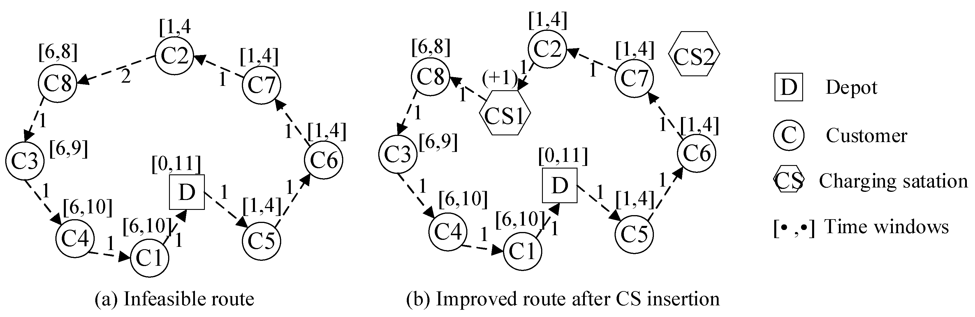
5.2.3. CS Insertion Operation

Following the operations of crossover and mutation, some of the current EV distribution routes are not feasible on the battery level of the EVs. The CSs should be inserted into the infeasible routes to reasonably repair the vehicle routes. The greedy charging strategy is introduced to make the route feasible by identifying the first customer with a negative battery level of the EV, and inserting a CS in the part of the route before that customer [47,60]. The insertion procedure is illustrated in Figure 3.

In Figure 3a, an infeasible route, including eight customers and one depot, is depicted. In Figure 3b, S1 is inserted between C2 and C8 by maintaining both time windows of the depot and the battery level of the EV feasibility. The detailed insertion procedure is shown in Algorithm 3.

Algorithm 3 CS insertion procedure

1. For each infeasible route

Repeat

2.    Identify the first customer with the negative battery level of the EV

3.    Search for all feasible insertion points according to time windows and battery level before the first customer

4.    Select a CS from the set of candidate CSs to insert

5.    For each candidate CS

6.       Calculate the sum of distances from CS to the previous customer and the next customer for each feasible insertion point as the distance increment

7.    End for

8.    For each feasible insertion point

9.       Compare the distance increments between the feasible insertion point and all candidate CSs

10.        Select the CS with the minimum distance increment to insert

11.        Calculate and compare the delivery cost increment for the CS insertion

12.    End for

13.    Determine the final insertion point with the minimum delivery cost increment and insert the selected CS for the route

14.  Until all of the delivery routes are feasible on the battery level of the EV

15. End for

In Algorithm 3, the main idea of the greedy charging strategy consists of determining the first customer in the infeasible route at which the EV arrives with a negative battery level and inserting the ‘‘best” (which increases the distance least) CS on the route between that customer and the previous one.

5.2.4. Elite Retention Mechanism

An elite retention mechanism is introduced to merge the parent population with the child population for the non-dominated sorting, which makes the search space larger [71,72]. Then, individuals with a higher priority are selected after generating the next generation of populations. Meanwhile, the crowding degree is applied to select individuals at the same level, which ensures that the good individuals can have a higher probability of being retained [63,71]. The specific elite retention mechanism is shown in Figure 4.

In Figure 4, Q_t is the child population, P_t is the parent population, and N is the set population size. The elite retention mechanism can be realized by the following steps:

Step 1: Combine the parent population with the child population to form a new population, and perform the non-dominant sorting to rank individuals.

Step 2: Place the non-dominant individuals of the different ranks into the new parent population based on the Pareto rank order

Step 3: Calculate the crowding distance for all individuals of rank k + 1 and arrange all individuals in a descending order by crowding distance. Eliminate all individuals with a rank greater than k + 1 if the conditions that the total number of individuals is less than N after all of the individuals of rank k are placed into the new parent set, and the total number of individuals is greater than N after all of the individuals of rank k + 1 are placed into the new parent set, are reached.

Step 4: Add individuals to the new parent population as in steps 2 and 3 until the number of individuals in the new parent population is equal to N, and eliminate the remaining individuals.

5.2.5. Elite Retention Mechanism

The non-dominance ranking is a concept based on the Pareto dominance, which facilitates the selection of more superior individuals [73,74]. The procedure of non-dominated sorting consists of three components: First, find all of the individuals in the population that have not been dominated, and deposit these individuals in Pareto rank 1. Second, deposit individuals that are dominated only by individuals in rank 1 into Pareto rank 2. Third, repeat until all individuals have been given a Pareto rank. The set of individuals with Pareto rank 1 is the Pareto optimal solutions, and the curve formed by these individuals is the Pareto front.

The crowding distance comparison is adopted to select better individuals from the same level of solutions [74,75]. The crowding distance is a measure of the density of individuals on the same Pareto front and can be calculated by using Equation (40)

$$di{s}_n(j)=\frac{f_n(j+1)-f_n(j-1)}{f_n{}^{\max }-f_n{}^{\min }}$$

(40)

where j + 1 and j − 1 are two adjacent individuals on the same Pareto front, and $f_n^{\max }$ and $f_n^{\min }$ are the maximum and minimum values of the objective function n, respectively.

6. Computational Experiments

In this section, the numerical experiments are presented to verify the proposed solution method for solving the CS-LRPTWRS. In Section 6.1, an algorithm comparison is conducted to demonstrate the superiority of the proposed hybrid algorithm in this study. In Section 6.2, an empirical study is introduced to test the validity and practical implications of the proposed methodology. In Section 6.3, the management insights of EVCS-LRPTWRS are summarized.

6.1. Algorithm Comparison

The multi-objective genetic algorithm (MOGA) [76], multi-objective particle swarm optimization (MOPSO) [77] algorithm, multi-objective ant colony optimization (MOACO) algorithm [78] have a good performance in solving multi-objective optimization problems. The three listed algorithms are adopted to compare with the proposed INSGA-II in this study, to verify its effectiveness and superiority. A set of 20 benchmark instances of the MDVRPTW collected from the network and emerging optimization research group, are modified to evaluate the performance of the proposed INSGA-II in solving the EVCS-LRPTWRS. In the algorithm comparison of the EVCS-LRPTWRS, the locations of the candidate CSs are generated by randomly selecting from the group of customers, and the service periods are determined based on the customer’s time windows. The characteristics of the modified instances, including the number of depots, the number of customers, the number of candidate CSs, the number of service periods, and the EV loading capacity are illustrated in

Table 5. Characteristics of the tested dataset.

Instances	Datasets	Number of Depots	Number of Customers	Number of CSs	Number of Periods	EV Capacity
1	Pr01_15CS_4W	4	48	15	4	200
2	Pr02_15CS_4W	4	96	15	4	195
3	Pr03_15CS_4W	4	144	15	4	190
4	Pr04_15CS_4W	4	192	15	4	185
5	Pr05_15CS_4W	4	240	15	4	180
6	Pr06_15CS_4W	4	288	15	4	175
7	Pr07_20CS_6W	6	72	20	6	200
8	Pr08_20CS_6W	6	144	20	6	190
9	Pr09_20CS_6W	6	216	20	6	180
10	Pr10_20CS_6W	6	288	20	6	170
11	Pr11_15CS_4W	4	48	15	4	200
12	Pr12_15CS_4W	4	96	15	4	195
13	Pr13_15CS_4W	4	144	15	4	190
14	Pr14_15CS_4W	4	192	15	4	185
15	Pr15_15CS_4W	4	240	15	4	180
16	Pr16_15CS_4W	4	288	15	4	175
17	Pr17_20CS_6W	6	72	20	6	200
18	Pr18_20CS_6W	6	144	20	6	190
19	Pr19_20CS_6W	6	216	20	6	180
20	Pr20_20CS_6W	6	288	20	6	170

.

The proposed INSGA-II is compared with the MOGA, MOPSO, and MOACO to solve the EVCS-LRPTWRS based on the datasets given in Table 5. The parameters used in the MOGA and INSGA-II are set as follows: population size pop_size = 100, selection probability p_s = 0.5, crossover probability p_c = 0.9, and mutation probability p_m = 0.1. The key parameters of the MOPSO are as follows: inertia weight w = 0.7, personal learning coefficient g₁ = 1, and global learning coefficient g₂ = 2. The parameters of the MOACO are as follows: pheromone importance a = 5, heuristic factor importance b = 5, pheromone evaporation coefficient c =0.5. In addition, the maximum iteration number of four algorithms is set as g_max = 500. The comparison results of the three algorithms containing the TOC, the number of used EVs, and the number of selected CSs are shown in

Table 6. Algorithm comparison results.

Instance	INSGA-II			MOGA			MOPSO			MOACO
	TOC (USD)	EVs	CSs	TOC (USD)	EVs	CSs	TOC (USD)	EVs	CSs	TOC (USD)	EVs	CSs
1	4953	3	4	5785	4	7	5355	4	4	6075	4	7
2	9062	7	6	10,051	8	9	9072	7	7	10,141	8	9
3	12,774	10	8	13,574	12	10	13,061	10	10	13,696	12	11
4	17,531	15	11	18,357	17	11	17,597	15	11	18,479	17	12
5	21,796	20	14	22,993	20	14	21,975	21	16	23,218	20	15
6	25,687	23	15	26,776	25	15	26,560	24	15	26,878	26	15
7	6931	4	3	8048	5	4	7499	4	3	8162	6	4
8	13,590	6	7	14,416	8	10	13,595	6	9	14,662	8	11
9	21,792	15	9	22,849	16	9	22,346	16	11	22,905	17	10
10	26,795	22	16	27,831	24	18	27,417	22	18	27,939	24	19
11	5062	4	4	5994	4	5	5598	5	4	6354	5	6
12	9278	7	7	9855	7	9	9554	7	7	10,101	8	10
13	12,377	11	8	13,081	12	8	12,548	12	9	13,407	12	10
14	17,942	14	11	18,614	14	12	18,581	14	11	18,680	14	13
15	22,188	20	13	23,190	20	13	22,715	20	15	23,555	21	14
16	25,725	22	15	26,794	23	16	25,726	23	15	26,970	24	16
17	7274	4	4	8208	5	5	7691	4	4	8269	6	6
18	13,579	7	8	14,769	9	10	14,076	8	9	14,991	9	12
19	22,193	15	10	23,308	15	13	22,257	15	10	23,479	15	14
20	26,841	21	15	27,527	21	16	27,126	22	16	27,628	22	16
Average	16,169	13	9	17,101	13	11	16,567	13	10	17,279	14	12
t-test				−22.75	−5.41	−5.15	−6.41	−3.94	−4.56	−24.71	−7.63	−7.76
p-value				1.51 × 10−15	1.35 × 10−5	2.84 × 10−5	1.89 × 10−6	4.37 × 10−4	3.83 × 10−4	3.30 × 10−16	1.69 × 10−7	1.30 × 10−7

. The optimization solutions (i.e., the TOC, the number of EVs, and the number of selected CSs) of each instance corresponding to the three algorithms are obtained from the Pareto fronts, and the different Pareto fronts can be evaluated by the bi-objective function value.

In Table 6, the reasonableness of the algorithm comparison is demonstrated by the significant difference between the computation results of the t-test and p-value. Based on the average values, the costs of the four algorithms are USD 16,169, USD 17,101, USD 16,567, and USD 17,279, and the numbers of the selected CSs are 9, 11, 10, and 12, respectively, indicating that the proposed algorithm performs better in terms of cost and number of selected CSs. According to the calculation results of each set of instances, the optimized number of used EVs corresponding to the INSGA-II is basically smaller than the number of used EVs corresponding to the other three algorithms. This notion means that the MOPSO, MOGA, and MOACO are inferior to the performance of the INSGA-II. Therefore, the INSGA-II proposed in this study is effective and has a better performance in the calculation of the large and medium-sized multi-objective EV routing optimization and CS location problems.

6.2. Empirical Study

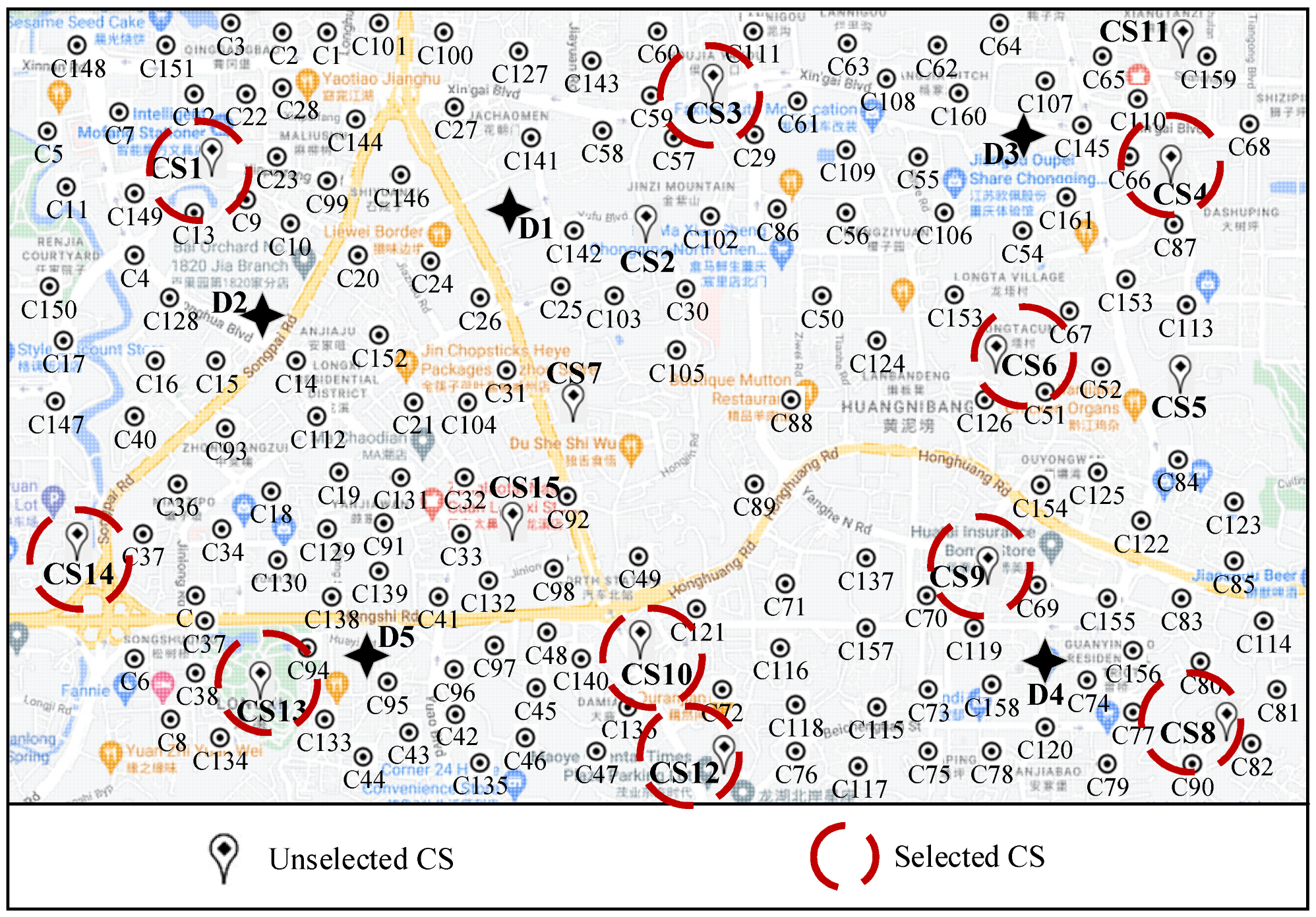
6.2.1. Data Source

An empirical study based on a real-world EV distribution network in Chongqing City, China is employed to test the applicability and effectiveness of the proposed solution methods (i.e., bi-objective nonlinear programming model, hybrid heuristic algorithm, and resource sharing strategy) in solving the EVCS-LRPTWRS. The EV distribution network is described in Figure 5 and

Table 7. Initial characteristics of the logistics network in the EVCS-LRPTWRS.

Depots	Customers	1st Period		2st Period
		Number of Services Customers	Time Windows	Number of Services Customers	Time Windows
D1	C1-C30	17	[0,10]	13	[12,24]
D2	C31-C65	19	[0,10]	16	[12,24]
D3	C66-C98	15	[0,10]	18	[12,24]
D4	C99-C132	20	[0,10]	14	[12,24]
D5	C133-C161	13	[0,10]	16	[12,24]
Total		84		77

.

In Figure 5 and Table 7, the EV distribution network is composed of five depots (D1, D2, D3, D4, and D5), a set of 15 candidate CSs (CS1, CS2,..., CS15), and 161 customers (C1, C2,..., C161). The depots are marked as black stars and have various service periods. The customers are served by the different logistic facilities in various service periods, and the candidate CSs can be simultaneously used by multiple EVs. The parameters used in the model formulation of the EVCS-LRPTWRS that can be set based on the related references [12,42] and actual surveys, are shown in

Table 8. Parameter settings of the model formulation in the EVCS-LRPTWRS.

Parameter	Description	Value
fe	Electricity price, (unit: USD/kWh)	1.8
Fcc	CC of electricity per unit time, (unit: USD/h)	4.5
FRr	Unit operating cost of CS	50
δv	Charging rate of EV v, v∈V, (unit: kWh/h)	25
μd	Variable cost coefficient of depot d, d∈D	0.4
MNv	Annual maintenance cost of EV v, v∈V	200
K	Number of working periods in one year	52
${\lambda }_t$	Arc specific coefficient of ET t, t∈T	0.13
${\gamma }_t$	Vehicle specific coefficient of ET t, t∈T	0.79
αv	Arc specific coefficient of EV v, v∈V	0.11
βv	Vehicle specific coefficient of EV v, v∈V	0.76
$S{V}_{vn}^w$	Driving speed of EV v in the nth route within the wth service period, v∈V, n∈$N_y^w$, w∈W, (unit: m/s)	11.11
$S{T}_{tm}^w$	Driving speed of EV v in the mth route within the wth service period, t∈T, m∈ $M_t^w$ w∈W, (unit: m/s)	11.11
$WE{V}_{vn}^w$	Weight of EV v in the nth route within the wth service period, v∈V, n∈$N_y^w$, w∈W, v∈V, (unit: kg)	1910
$WE{T}_{tm}^w$	$\mathrm{Weight} \mathrm{of} \mathrm{ET} t \mathrm{in} \mathrm{the} m\mathrm{th} \mathrm{route} \mathrm{within} \mathrm{the} w\mathrm{th} \mathrm{service} \mathrm{period}, t\in T, m\in M_t^w$, w∈W, v∈V, (unit: kg)	4000
QTt	Load capacity of ET t, t∈T	1000
QVv	Load capacity of EV v, v∈V	600
Pe	PC per unit of time of earliness	4
Pl	PC per unit of time of delay	8
Ev	Battery capacity of EV v, v∈V, (unit: kWh)	48

.

6.2.2. Optimization Results

(1)

Customer clustering results

Customers are clustered by the Gaussian hybrid clustering algorithm according to their coordinates and time windows in order to simplify the computational complexity of the EVCS-LRPTWRS and to determine the number of service periods. Every customer can be reassigned to the depot service with a certain probability with the cooperation of multiple depots and customer service sharing. The clustering results are shown in Figure 6.

In Figure 6, customers with similar characteristics are divided into a cluster. A customer will be assigned to a depot based on the geographic coordinates and time windows of the customer. For example, customers assigned to D3 are represented by blue balls. Meanwhile, customers assigned to D4 are represented by green balls. These customers are classified into two tiers. The lower and upper layers represent the customers to be served in the first and second service periods, respectively. In summary, different customers will be served by the corresponding depots in different service periods.

(2)

CS location and the routing optimization results

Based on the previous customer clustering results, the CS selection strategy in each service period is performed by selecting the appropriate CSs for all of the delivery routes that need to be inserted CSs for EVs.

Table 9. CS location selection results of the various depots.

Depots	1st	2nd	CS Location
D1	CS1	CS1	CS1, CS3, CS4 CS6, CS8, CS9, CS10 CS12, CS13, CS14
D2	CS13, CS14	CS1, CS14
D3	CS3, CS4	CS3, C6
D4	CS6, CS9, CS12	CS8, CS10
D5	CS10, CS13	CS10

and Figure 7 show the CS location selection strategies for the two service periods.

In Table 9 and Figure 7, a total of ten CSs are selected for charging by the EVs, namely, CS1, CS3, CS4, CS6, CS8, CS9, CS10, CS12, CS13, and CS14. In the first service period, all nine CSs are used by the EVs. Meanwhile, only six CSs are used by the EVs in the second service period. Some CSs are shared in different depots and service periods in the same depot. For example, CS1 is shared by D1 in periods 1 and 2, and CS10 is shared between D4 and D5 in period 2.

Table 10. Optimization results of the EVCS-LRPTWRS.

Case	Service Period	EC (kWh)	EDC (USD)	CC (USD)	PC (USD)	CTC (USD)	DOC (USD)	COC (USD)	TOC (USD)	Used EVs	Shared Routes	ETs	Used CSs
Initial	1st	3569	6424	197	286	0	500	0	10,976	19	0	0	8
	2nd	2770	4986	108	154	0	500	0	8518	13	0	0	7
	Total	6339	11,410	305	440	0	1000	0	19,494	32	0	0	15
Optimized	1st	2653	4775	162	107	237	536	300	8770	9	7	1	9
	2nd	2178	3920	83	96	186	513	200	7176	5	5	1	7
	Total	4853	8695	245	203	423	1049	500	15,968	9	12	1	10

and Figure 8 summarize the optimization results of the EVCS-LRPTWRS, including the electricity consumption (EC), electric delivery cost (EDC), charging cost (CC), penalty cost (PC), centralized transportation cost (CTC), the operating cost of depots (DOC), the operating cost of CSs (COC), the total operating cost (TOC), the number of used EVs (Used EVs), the number of shared routes (Shared routes), and the number of selected CS locations (Used CSs).

In Table 10 and Figure 8, the EC, PC, TOC, the number of selected CSs, and the number of used EVs in both two service periods present a downward trend compared with the initial logistics network. The TOC is reduced from USD 19,494 to USD 15,968 with the vehicle routing optimization, a decrease of 18%. The EC dropped from 6339 kWh to 4853 kWh, thereby obtaining 1986 kWh of electricity savings. The PCs decreased from USD 440 to USD 203, indicating that the violations of customers’ time windows are alleviated. Furthermore, the number of selected CSs dropped from 15 to 10 and the number of used EVs shifted from 32 to 9 with the implementation of the transportation resource sharing strategy. The delivery routes from the depots to their service customers can be optimized and reconstructed by the proposed INSGA-II described in Section 5.2. The further optimization results of the scheme of the delivery routes and the transportation resource sharing strategies for the EVCS-LRPTWRS are shown in

Table 11. Optimized routes of EVCS-LRPTWRS.

Depot	EV	Service Period	Route
D1	EV1	1st	C24→C152→C26→C104→C31→C105→C103→C25→C142
	EV2	1st	C27→C100→C101→C1→C28→C2→C3→C151→C12→CS1→C9→C10→C99→C144→C146
	EV1	1st	C58→C59→C143→C141
	EV4	2nd	C21→C112→C14→C20→C23→CS1→C22→C127
D2	EV3	1st	C4→C11→C149→C5→C148→C7
	EV4	1st	C34→C36→C39→CS13→C38→C8→C6→C37→CS14→C40→C147→C150
	EV5	2nd	C15→C93→CS13→C134→CS14→C17→C16→C128→C13
D3	EV3	1st	C106→C153→C67→C161→C66→C68→CS4→C159→C65→C110→C145
	EV7	1st	C107→C64→C62→C108→C109→C61→C29→CS3→C30→C102→C60→CS3→C63→C160
	EV8	2nd	C54→C87→C113→C53→CS6→C124→C50→C86→CS3→C57→C111→C56→C55
D4	EV9	1st	C158→C73→C157→C72→C71→C137→C70→CS9→C69→C154→C155→C156→C74
	EV8	1st	C119→C125→C52→C51→C126→CS6→C88→C89→C121→CS12→C76→C118→C116→C115→C117→C75
	EV1	2nd	C120→C77→C79→C90→C82→CS8→C81→C114→C85→C123→C84→C122→C83→C80
D5	EV5	1st	C43→C44→C42→C135→C136→C140→CS10→C96→C139
	EV6	1st	C94→C133→C138→CS13→C35→C32→C33→C98→C97→C41→C95
	EV3	2nd	C46→C47→C45→C48→CS10→C49→C92→C132→C91→C131→C19→C129→C18→C130

CS: Charging stations selected in the routes.

and Figure 9.

In Table 11 and Figure 9, nine EVs perform a total of 16 routes for delivery tasks. Eleven delivery routes are executed by nine EVs in the first service period, and five de-livery routes are completed by three EVs in the second service period. Each EV can be shared within a service period and among several service periods with the implementation of the transportation resource sharing strategy. For example, EV1 initially serves nine customers and then serves four customers for the same depot in the first service period, and it continues to complete one delivery route for D4 in the second service period. The start and end times of the three shared routes do not overlap. Therefore, EV1 executes a total of three delivery routes and serves 26 customers, thereby realizing the sharing of transportation resources and greatly improving the utilization of EVs.

6.2.3. Analysis and Discussion

(1)

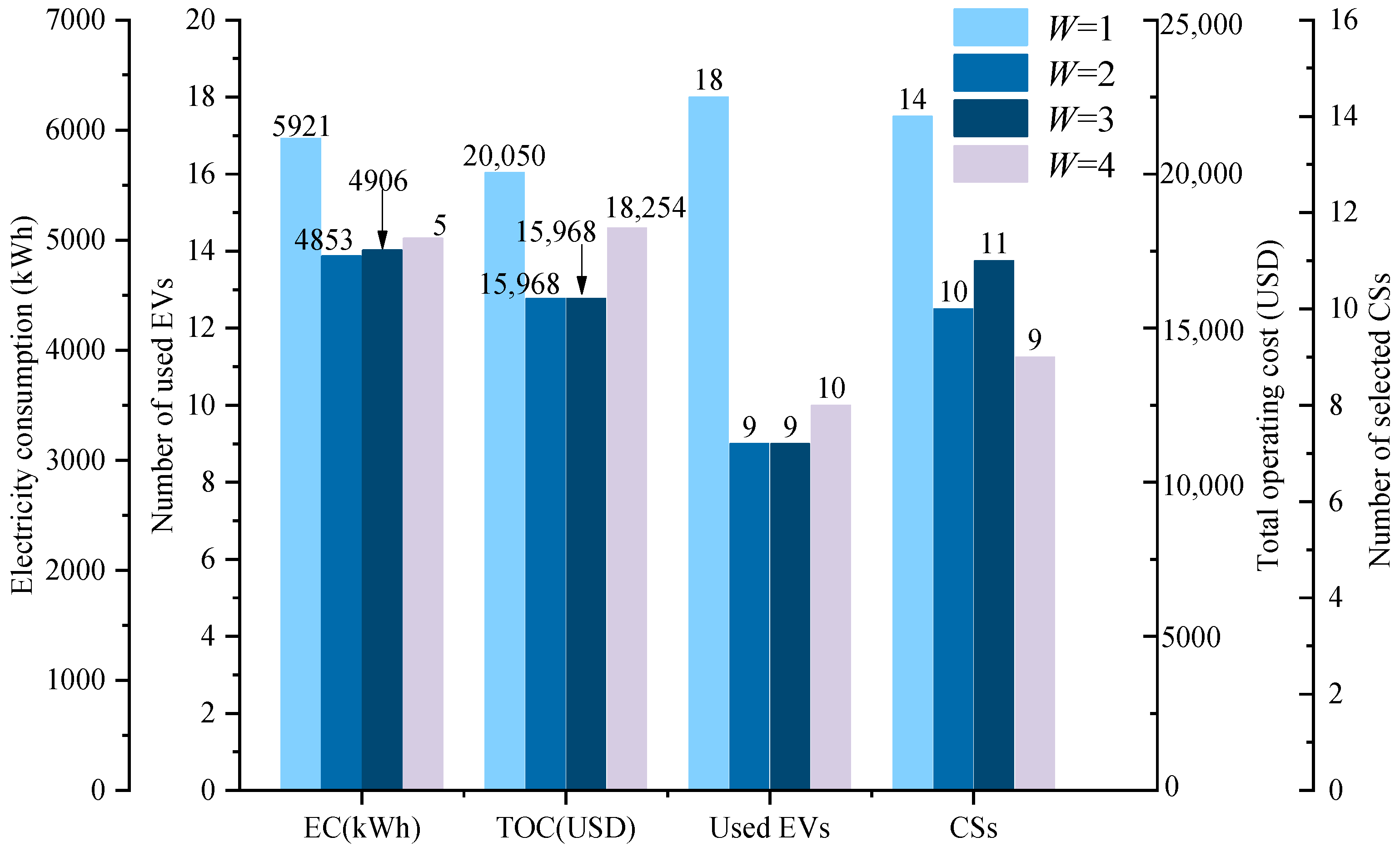
Comparison of the different service periods

The determination of the different number of service periods has an impact on the effect of optimization for EV distribution networks. This section demonstrates the applicability of the service periods in the EVCS-LRPTWRS optimization by further analyzing the determination of service periods. The optimization results under different values of W are compared to determine the optimal number of service periods. The comparison results are shown in

Table 12. Comparison results of the different service periods.

Service Periods	W = 1				W = 2				W = 3				W = 4
	EC	TOC (USD)	EVs	CSs	EC	TOC (USD)	EVs	CSs	EC	TOC (USD)	EVs	CSs	EC	TOC (USD)	EVs	CSs
1st	5921	20,050	18	14	2653	8770	9	9	1829	6351	8	11	1537	5276	7	7
2nd	/	/	/	/	2178	7176	5	7	1594	5413	4	6	1320	4658	4	6
3rd	/	/	/	/	/	/	/	/	1483	4974	3	6	1176	4366	4	5
4th	/	/	/	/	/	/	/	/	/	/	/	/	980	3954	3	5
Total	5921	20,050	18	14	4853	15,968	9	10	4906	16,738	9	11	5013	18,254	10	9
Selected CS locations	CS1, CS2, CS3, CS4 CS6, CS7, CS8, CS9, CS10, CS11, CS12, CS13, CS14, CS15				CS1, CS3, CS4 CS6, CS8, CS9, CS10 CS12, CS13, CS14				CS1, CS2, CS3, CS4 CS6, CS9, CS10, CS12 CS13, CS14, CS15				CS1, CS3, CS4 CS6, CS8, CS9, CS10 CS13, CS14

and Figure 10.

The optimization results, including the EC, TOC, the number of EVs, and the number of selected CS locations under various service period segmentation scenarios are shown in Table 12 and Figure 10. Compared with the EC of 5921kWh, the TOC of USD 20,050, 18 EVs in demand, and 14 selected CSs without period segmentation, the corresponding indicators for the other three scenarios with a service period segmentation are significantly reduced. When W = 2, the minimum the TOC can reach USD 15,968, which is reduced by USD 770 and USD 2286 compared with those of W = 3 and W = 4, and no significant gap is observed in the number of EVs and selected CSs. Therefore, dividing the entire work period into two service periods in the empirical study is the optimal choice from the perspective of the bi-objective of minimizing the cost and number of vehicles.

(2)

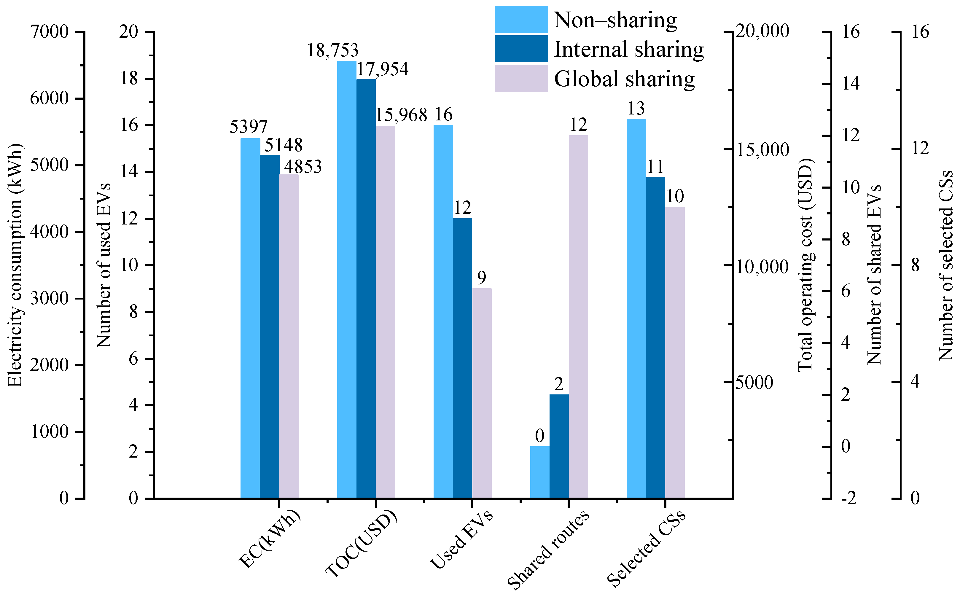
Comparison of different resource sharing strategies

Three scenarios of EV sharing are considered based on the EV routing optimization and the CS location selection analysis for two service periods to prove the effectiveness and practicality of the transportation resource sharing strategy: (1) non-sharing of EVs in the EV distribution network; (2) internal sharing of EVs in the EV distribution network among various periods in the same depot; and (3) global sharing of EVs in the EV distribution network among various periods or different depots. The comparison results of the number of used EVs, the number of shared routes, the EC, the TOC, and the number of the selected CSs under the three sharing modes are shown in

Table 13. Comparison results of the three cases of the resource sharing strategy.

Case	Service Period	EC (kWh)	TOC (USD)	Used EVs	Shared Routes	Selected CSs
Non-sharing	1st	2936	9755	10	0	10
	2nd	2461	8998	6	0	7
	Total	5397	18,753	16	0	13
Internal sharing	1st	2722	9406	10	1	10
	2nd	2426	8548	6	1	7
	Total	5148	17,954	12	2	11
Global sharing	1st	2653	8770	9	7	9
	2nd	2178	7176	5	5	7
	Total	4853	15,968	9	12	10

and Figure 11.

In Table 13 and Figure 11, the TOC is decreased from USD 18,753 to USD 17,954 to USD 15,968 as the number of shared routes is increased from the non-sharing of zero to the internal sharing of two to the global sharing of 12, and the number of used EVs is declined from 16 to 12 to 9. Moreover, the EC and the number of selected CSs are decreasing with the deepening of the transportation resource sharing strategy. The minimum number of used EVs, the maximum number of shared routes, and the lowest TOC in the third case prove that the global sharing model is the optimal transportation resource sharing model. Therefore, the transportation resource sharing strategy is conducive to saving transportation resources and optimizing the resource allocation, thus achieving a reduction in the TOC and an increase in the transportation efficiency.

6.3. Management Insights

A transportation resource sharing strategy is incorporated into the optimization of the CS location-routing problem for a multi-depot multi-period EV distribution network. The reduction of the TOC and the improvement of transportation efficiency demonstrate the benefits of addressing the EVCS-LRPTWRS. In this section, the management insights of this study are described as follows:

(1)

This study has a significant practical implication for the optimization of logistics networks. The periodic location selections of CSs contribute to promoting delivery efficiency via the reassignment of customers according to their characteristics in different service periods. The optimization of the EV delivery routes greatly alleviates the phenomenon of long-distance transportation and violations of customers’ time windows. The adoption of a transportation resource sharing strategy in a multi-depot multi-period EV distribution network can reduce the number of required EVs, thus facilitating the construction of resource-efficient and environmentally friendly logistics networks.

(2)

The proposed solution method in this study to solve the EVCS-LRPTWRS can provide a methodological reference for the research of the EVLRP. The bi-objective nonlinear programming model of the minimum TOC and the minimum number of required EVs balances the operation of the logistics network from two conflicting aspects of economy and efficiency. In addition, the hybrid algorithm, including a customer clustering algorithm and a heuristic algorithm, is developed to solve the EVCS-LRPTWRS. The service periods are divided by customer clustering according to the time window’s characteristics for improving the transportation efficiency. The integration of the CS insertion operation into the heuristic algorithm allows for the reasonable CS location, thus, shortening the delivery distance and saving the operating cost. Therefore, the proposed solution methods contribute to building an economic and sustainable logistics network and promoting the enterprise’s competitiveness.

(3)

The optimization of the EV distribution networks plays a great role in alleviating the conflicts between humans and the environment. With the proposal of the dual-carbon goal: carbon peak and carbon neutrality, EVs are widely adopted by enterprises and logistics companies to construct a sustainable logistics distribution network for coping with the increasing competition. Meanwhile, many government departments have enacted a series of policies to promote the popularity and development of EVs to face the two challenges of environmental degradation and energy scarcity. Furthermore, new energy technologies (e.g., vehicle-pile cloud interconnection, wireless charging, and power exchange technology) should be widely promoted to address the technical limitations and practical application constraints of EVs.

7. Conclusions

This study proposes a problem of the EVCS-LRPTWRS to simultaneously determine the locations of CSs and optimize the route plans of EVs. A resource sharing strategy among multiple depots within the various service periods is introduced to improve the operational efficiency of the logistics networks and rationalize resource configuration. First, a bi-objective nonlinear programming model is formulated to minimize the TOC and the number of EVs. Second, a hybrid algorithm combining the GMCA and INSGA-II is developed to achieve the Pareto optimal solutions of the proposed problem. Third, an algorithm comparison between the INSGA-II and three other algorithms (e.g., MOGA, MOPSO, and MOACO) is carried out to test the performance of the proposed algorithm. Finally, an empirical study of Chongqing City, China is designed to verify the validity and practicality of the proposed model and algorithm. In addition, the sensitivity analyses of the service periods and sharing modes are explored and discussed to demonstrate the effectiveness of the proposed strategies.

The comparison results between the proposed INSGA-II and MOGA, and MOPSO have demonstrated the superiority of the proposed algorithm in optimizing the EVCS-LRPTWRS. In a real-world case study, the TOC is reduced by USD12,047, the number of EVs is decreased by 29, the selected CS locations is minimized from 15 to 10, and the EC of EVs is dropped by 1348 kWh after the optimization of the initial logistics network. The effectiveness and practicality of the proposed solution methods in reducing the operating costs, number of EVs, and EC in the EVCS-LRPTWRS are proven by the experimental calculation results. The different service period divisions indicate that dividing the whole working period into two service periods is the optimal period classification. In addition, three modes of resource sharing strategy are analyzed and discussed, and the comparison results illustrate that the global sharing of EVs is superior to the other modes. These findings show that the transportation resource sharing among multiple depots within various service periods is an economical and efficient strategy to construct sustainable logistics networks.

This study has significant implications for academic researchers and logistics enterprises. The transportation resource sharing strategy and service period division are incorporated in the selection of CS locations. Future research can be considered in the following directions: (1) More constraints (i.e., the capacity of CSs, the nonlinearity of charging speed, and the influence of cargo loading) can be considered to extend the practicality of the mathematical model. (2) Pickup and delivery services can be incorporated into future studies of the EVLRP, and the synchronization and coordination of the two activities can be deepened. (3) Dynamics and uncertainty of customer demands can be further studied in the EVCS-LRPTWRS to fit the actual logistics network considerations. (4) The mode of transportation resource sharing strategy is worth further exploring to optimize the resource configuration and improve the transportation efficiency in the logistics network.

References

1. Yang, S.Y.; Ning, L.J.; Tong, L.; Shang, P. Integrated electric logistics vehicle recharging station location–routing problem with mixed backhauls and recharging strategies. Transp. Res. Part C Emerg. Technol. 2022, 140, 103605. [Google Scholar] [CrossRef]
2. Asadi, S.; Nilashi, M.; Iranmanesh, M.; Ghobakhloo, M.; Samad, S.; Alghamdi, A.; Almulihi, A.; Mohd, S. Drivers and barriers of electric vehicle usage in Malaysia: A DEMATEL approach. Resour. Conserv. Recycl. 2022, 177, 105965. [Google Scholar] [CrossRef]
3. Wang, L.; Gao, S.; Wang, K.; Li, T.; Li, L.; Chen, Z.Y. Time-dependent electric vehicle routing problem with time Windows and path flexibility. J. Adv. Transp. 2020, 2020, 3030197. [Google Scholar] [CrossRef]
4. Kchaou-Boujelben, M. Charging station location problem: A comprehensive review on models and solution approaches. Transp. Res. Part C Emerg. Technol. 2021, 132, 103376. [Google Scholar] [CrossRef]
5. Li, J.Q.; Han, Y.Q.; Duan, P.Y.; Han, Y.Y.; Niu, B.; Li, C.D.; Zheng, Z.X.; Liu, Y.P. Meta-heuristic algorithm for solving vehicle routing problems with time windows and synchronized visit constraints in prefabricated systems. J. Clean. Prod. 2020, 250, 119464. [Google Scholar] [CrossRef]
6. Chen, R.; Liu, X.L.; Mia, L.X.; Yang, P. Electric vehicle tour planning considering range anxiety. Sustainability 2020, 9, 3685. [Google Scholar] [CrossRef]
7. Schiffer, M.; Walther, G. The electric location routing problem with time windows and partial recharging. Eur. J. Oper. Res. 2017, 260, 995–1013. [Google Scholar] [CrossRef]
8. Ran, C.; Zhang, Y.; Yin, Y. Demand response to improve the shared electric vehicle planning: Managerial insights, sustainable benefits. Appl. Energy 2021, 292, 112863. [Google Scholar] [CrossRef]
9. Li, J.L.; Liu, Z.B.; Wang, X.F. Public charging station location determination for electric ride-hailing vehicles based on an improved genetic algorithm. Sustain. Cities Soc. 2021, 74, 103182. [Google Scholar] [CrossRef]
10. He, P.; Zhang, S.S.; He, C. Impacts of logistics resource sharing on B2C E-commerce companies and customers. Electron. Commer. Res. Appl. 2019, 34, 100820. [Google Scholar] [CrossRef]
11. Xu, X.F.; Hao, J.; Zheng, Y. Multi-objective artificial bee colony algorithm for multi-stage resource leveling problem in sharing logistics network. Comput. Ind. Eng. 2020, 142, 106338. [Google Scholar] [CrossRef]
12. Wang, Y.; Sun, Y.Y.; Guan, X.Y.; Fan, J.X.; Xu, M.Z.; Wang, H.Z. Two-echelon multi-period location routing problem with shared transportation resource. Knowl. Based Syst. 2021, 226, 107168. [Google Scholar] [CrossRef]
13. Wang, Y.; Assogba, K.; Fan, J.X.; Xu, M.Z.; Liu, Y.; Wang, H.Z. Multi-depot green vehicle routing problem with shared transportation resource: Integration of time-dependent speed and piecewise penalty cost. J. Clean. Prod. 2019, 232, 12–29. [Google Scholar] [CrossRef]
14. Erdelić, T.; Carić, T. A Survey on the electric vehicle routing problem: Variants and solution approaches. J. Adv. Transp. 2019, 2019, 5075671. [Google Scholar] [CrossRef]
15. Ghorbani, E.; Alinaghian, M.; Gharehpetian, G.B.; Mohammadi, S.; Perboli, G. A survey on environmentally friendly vehicle routing problem and a proposal of its classification. Sustainability 2020, 12, 9079. [Google Scholar] [CrossRef]
16. Kucukoglu, I.; Dewil, R.; Cattrysse, D. The electric vehicle routing problem and its variations: A literature review. Comput. Ind. Eng. 2021, 161, 107650. [Google Scholar] [CrossRef]
17. Dündar, H.; Ömürgönülşen, M.; Soysal, M. A review on sustainable urban vehicle routing. J. Clean. Prod. 2021, 285, 125444. [Google Scholar] [CrossRef]
18. Qin, H.; Su, X.X.; Ren, X.; Luo, Z.X. A review on the electric vehicle routing problems: Variants and algorithms. Front. Eng. Manag. 2021, 8, 370–389. [Google Scholar] [CrossRef]
19. Xiao, Y.Y.; Zhang, Y.; Kaku, I.; Kang, R.; Pan, X. Electric vehicle routing problem: A systematic review and a new comprehensive model with nonlinear energy recharging and consumption. Renew. Sustain. Energy Rev. 2021, 151, 111567. [Google Scholar] [CrossRef]
20. Paz, J.C.; Granada-Echeverri, M.; Escobar, J.W. The multi-depot electric vehicle location routing problem with time windows. Int. J. Ind. Eng. Comput. 2018, 9, 123–136. [Google Scholar] [CrossRef]
21. Yang, J.; Sun, H. Battery swap station location-routing problem with capacitated electric vehicles. Comput. Oper. Res. 2015, 55, 217–232. [Google Scholar] [CrossRef]
22. Yidiz, B.; Arslan, O.; Karasan, O.E. A branch and price approach for routing and refueling station location model. Eur. J. Oper. Res. 2016, 248, 815–826. [Google Scholar] [CrossRef]
23. He, J.; Yang, H.; Tang, T.Q.; Huang, H.J. An optimal charging station location model with the consideration of electric vehicle’s driving range. Transp. Res. Part C Emerg. Technol. 2018, 86, 641–654. [Google Scholar] [CrossRef]
24. Zhang, S.; Chen, M.Z.; Zhang, W.Y. A novel location-routing problem in electric vehicle transportation with stochastic demands. J. Clean. Prod. 2019, 221, 567–581. [Google Scholar] [CrossRef]
25. Guo, F.; Huang, Z.H.; Huang, W.L. Integrated location and routing planning of electric vehicle service stations based on users’ differentiated perception under a time-sharing leasing mode. J. Clean. Prod. 2020, 277, 123513. [Google Scholar] [CrossRef]
26. Calik, H.; Oulamara, A.; Prodhon, C.; Salhi, S. The electric location-routing problem with heterogeneous fleet: Formulation and Benders decomposition approach. Comput. Oper. Res. 2021, 131, 105251. [Google Scholar] [CrossRef]
27. Wang, C.L.; Guo, C.C.; Zuo, X.Q. Solving multi-depot electric vehicle scheduling problem by column generation and genetic algorithm. Appl. Soft Comput. 2021, 112, 107774. [Google Scholar] [CrossRef]
28. Sadati, M.E.H.; Catay, B. A hybrid variable neighborhood search approach for the multi-depot green vehicle routing problem. Transp. Res. Part E Logist. Transp. Rev. 2021, 149, 102293. [Google Scholar] [CrossRef]
29. Lam, E.; Desaulniers, G.; Stuckey, P.J. Branch-and-cut-and-price for the electric vehicle routing problem with time windows, piecewise-linear recharging and capacitated recharging stations. Comput. Oper. Res. 2022, 145, 105870. [Google Scholar] [CrossRef]
30. Raeesi, R.; Zografos, K.G. The electric vehicle routing problem with time windows and synchronised mobile battery swapping. Transportation Res. Part B Methodol. 2020, 140, 101–129. [Google Scholar] [CrossRef]
31. Li, S.Y.; Huang, Y.X.; Mason, S.J. A multi-period optimization model for the deployment of public electric vehicle charging stations on network. Transp. Res. Part C Emerg. Technol. 2016, 65, 128–143. [Google Scholar] [CrossRef]
32. Neves-Moreira, F.; Amorim-Lopes, M.; Amorim, P. The multi-period vehicle routing problem with refueling decisions: Traveling further to decrease fuel cost. Transp. Res. Part E Logist. Transp. Rev. 2017, 133, 101817. [Google Scholar] [CrossRef]
33. Lin, B.; Ghaddar, B.; Nathwani, J. Electric vehicle routing with charging/discharging under time-variant electricity prices. Transp. Res. Part C Emerg. Technol. 2021, 130, 103285. [Google Scholar] [CrossRef]
34. Brandstätter, G.; Kahr, M.; Leitner, M. Determining optimal locations for charging stations of electric car-sharing systems under stochastic demand. Transp. Res. Part B Methodol. 2017, 104, 17–35. [Google Scholar] [CrossRef]
35. Friedrich, M.; Noekel, K. Modeling intermodal networks with public transport and vehicle sharing systems. EURO J. Transp. Logist. 2017, 6, 271–288. [Google Scholar] [CrossRef]
36. Almouhanna, A.; Quintero-Araujo, C.L.; Panadero, J.; Juan, A.A.; Khosravi, B.; Ouelhadj, D. The location routing problem using electric vehicles with constrained distance. Comput. Oper. Res. 2020, 115, 104864. [Google Scholar] [CrossRef]
37. Jin, F.; Yao, E.; An, K. Analysis of the potential demand for battery electric vehicle sharing: Mode share and spatiotemporal distribution. J. Transp. Geogr. 2020, 82, 102630. [Google Scholar] [CrossRef]
38. Chen, Y.R.; Li, D.C.; Zhang, Z.C.; Wahab, M.I.M.; Jiang, Y.S. Solving the battery swap station location-routing problem with a mixed fleet of electric and conventional vehicles using a heuristic branch-and-price algorithm with an adaptive selection scheme. Expert Syst. Appl. 2021, 186, 115683. [Google Scholar] [CrossRef]
39. Yang, Y.; He, K.; Wang, Y.P.; Yuan, Z.Z.; Yin, Y.H.; Guo, M.Z. Identification of dynamic traffic crash risk for cross-area freeways based on statistical and machine learning methods. Phys. A Stat. Mech. Its Appl. 2022, 595, 127083. [Google Scholar] [CrossRef]
40. Bayliss, C. Machine learning based simulation optimisation for urban routing problems. Appl. Soft Comput. 2021, 105, 107269. [Google Scholar] [CrossRef]
41. Yang, Y.; Yuan, Z.Z.; Chen, J.J.; Guo, M.Z. Assessment of osculating value method based on entropy weight to transportation energy conservation and emission reduction. Environ. Eng. Manag. J. 2017, 16, 2413–2423. [Google Scholar] [CrossRef]
42. Yang, Y.; Wang, K.; Yuan, Z.Z.; Liu, D. Predicting freeway traffic crash severity using XGBoost-Bayesian network model with consideration of features interaction. J. Adv. Transp. 2022, 2022, 4257865. [Google Scholar] [CrossRef]
43. Barco, J.; Guerra, A.; Munoz, L.; Quijano, N. Optimal routing and scheduling of charge for electric vehicles: A case study. Math. Probl. Eng. 2017, 2017, 1–16. [Google Scholar] [CrossRef]
44. Kyriakakis, N.A.; Stamadianos, T.; Marinaki, M.; Marinakis, Y. The electric vehicle routing problem with drones: An energy minimization approach for aerial deliveries. Clean. Logist. Supply Chain 2022, 4, 100041. [Google Scholar] [CrossRef]
45. Zhang, H.; Tang, L.; Yang, C.; Lan, S.L. Locating electric vehicle charging stations with service capacity using the improved whale optimization algorithm. Adv. Eng. Inform. 2019, 41, 100901. [Google Scholar] [CrossRef]
46. Yu, V.F.; Jodiawan, P.; Gunawan, A. An Adaptive Large Neighborhood Search for the green mixed fleet vehicle routing problem with realistic energy consumption and partial recharges. Appl. Soft Comput. 2021, 105, 107251. [Google Scholar] [CrossRef]
47. Erdem, M. Optimisation of sustainable urban recycling waste collection and routing with heterogeneous electric vehicles. Sustain. Cities Soc. 2022, 80, 103785. [Google Scholar] [CrossRef]
48. Breunig, U.; Baldacci, R.; Hartl, R.F.; Vidal, T. The electric two-echelon vehicle routing problem. Comput. Oper. Res. 2019, 103, 198–210. [Google Scholar] [CrossRef]
49. Chakraborty, N.; Mondal, A.; Mondal, S. Intelligent charge scheduling and eco-routing mechanism for electric vehicles: A multi-objective heuristic approach. Sustain. Cities Soc. 2021, 69, 102820. [Google Scholar] [CrossRef]
50. Felipe, Á.; Ortuño, M.T.; Righini, G.; Tirado, G. A heuristic approach for the green vehicle routing problem with multiple technologies and partial recharges. Transp. Res. Part E Logist. Transp. Rev. 2014, 71, 111–128. [Google Scholar] [CrossRef]
51. Froger, A.; Mendoza, J.E.; Jabali, O.; Laporte, G. Improved formulations and algorithmic components for the electric vehicle routing problem with nonlinear charging functions. Comput. Oper. Res. 2019, 104, 256–294. [Google Scholar] [CrossRef]
52. Jie, W.C.; Yang, J.; Zhang, M.; Huang, Y.X. The two-echelon capacitated electric vehicle routing problem with battery swapping stations: Formulation and efficient methodology. Eur. J. Oper. Res. 2019, 272, 879–904. [Google Scholar] [CrossRef]
53. Hof, J.; Schneider, M.; Goeke, D. Solving the battery swap station location-routing problem with capacitated electric vehicles using an AVNS algorithm for vehicle-routing problems with intermediate stops. Transportation Res. Part B Methodol. 2017, 97, 102–112. [Google Scholar] [CrossRef]
54. Ma, B.S.; Hu, D.W.; Chen, X.Q.; Wang, Y.; Wu, X. The vehicle routing problem with speed optimization for shared autonomous electric vehicles service. Comput. Ind. Eng. 2021, 161, 102214. [Google Scholar] [CrossRef]
55. Pelletier, S.; Jabali, O.; Laporte, G. The electric vehicle routing problem with energy consumption uncertainty. Transp. Res. Part B Methodol. 2019, 126, 225–255. [Google Scholar] [CrossRef]
56. Zhu, Z.H.; Gao, Z.Y.; Zheng, J.F.; Du, H.M. Charging station location problem of plug-in electric vehicles. J. Transp. Geogr. 2016, 52, 11–22. [Google Scholar] [CrossRef]
57. Keskin, M.; Çatay, B. Partial recharge strategies for the electric vehicle routing problem with time windows. Transp. Res. Part C Emerg. Technol. 2016, 65, 111–127. [Google Scholar] [CrossRef]
58. Cataldo-Diaz, C.; Linfati, R.; Escobar, J.W. Mathematical model for the electric vehicle routing problem considering the state of charge of the batteries. Sustainability 2022, 3, 1645. [Google Scholar] [CrossRef]
59. Wang, Y.; Li, Q.; Guan, X.Y.; Fan, J.X.; Liu, Y.; Wang, H.Z. Collaboration and resource sharing in the multidepot multiperiod vehicle routing problem with pickups and deliveries. Sustainability 2020, 12, 5966. [Google Scholar] [CrossRef]
60. Li, J.J.; Fang, Y.H.Q.; Tang, N. A cluster-based optimization framework for vehicle routing problem with workload balance. Comput. Ind. Eng. 2022, 169, 108221. [Google Scholar] [CrossRef]
61. Chen, Q.; Pan, X.Y.; Liu, F.; Xiong, Y.; Li, Z.T.; Tang, J.J. Reposition optimization in free-floating bike-sharing system: A case study in Shenzhen City. Phys. A Stat. Mech. Its Appl. 2022, 593, 126925. [Google Scholar] [CrossRef]
62. Tang, J.J.; Hu, J.; Hao, W.; Chen, X.Q.; Qi, Y. Markov Chains based route travel time estimation considering link spatio-temporal correlation. Phys. A Stat. Mech. Its Appl. 2020, 545, 123759. [Google Scholar] [CrossRef]
63. Liao, W.Z.; Zhang, L.Y.; Wei, Z.Z. Multi-objective green meal delivery routing problem based on a two-stage solution strategy. J. Clean. Prod. 2020, 258, 120627. [Google Scholar] [CrossRef]
64. Eydi, A.; Ghasemi-Nezhad, S.A. A bi-objective vehicle routing problem with time windows and multiple demands. Ain Shams Eng. J. 2021, 12, 2617–2630. [Google Scholar] [CrossRef]
65. Srivastava, G.; Singh, A.; Mallipeddi, R. NSGA-II with objective-specific variation operators for multiobjective vehicle routing problem with time windows. Exp. Syst. Appl. 2021, 176, 114779. [Google Scholar] [CrossRef]
66. Katoch, S.; Chauhan, S.S.; Kumar, V. A review on genetic algorithm: Past, present, and future. Multimed. Tools Appl. 2021, 5, 8091–8126. [Google Scholar] [CrossRef]
67. Wang, Y.; Zhang, S.L.; Assogba, K.; Fan, J.X.; Xu, M.Z.; Wang, Y.H. Economic and environmental evaluations in the two-echelon collaborative multiple centers vehicle routing optimization. J. Clean. Prod. 2018, 197, 443–461. [Google Scholar] [CrossRef]
68. Li, Q.; Cao, Z.H.; Ding, W.P.; Li, Q. A multi-objective adaptive evolutionary algorithm to extract communities in networks. Swarm Evol. Comput. 2020, 52, 100629. [Google Scholar] [CrossRef]
69. Khoo, T.S.; Mohammad, B.B. The parallelization of a two-phase distributed hybrid ruin-and-recreate genetic algorithm for solving multi-objective vehicle routing problem with time windows. Expert Syst. Appl. 2021, 168, 14408. [Google Scholar] [CrossRef]
70. Koohestani, B. A crossover operator for improving the efficiency of permutation-based genetic algorithms. Expert Syst. Appl. 2020, 151, 113381. [Google Scholar] [CrossRef]
71. Wang, Y.; Wang, X.W.; Guan, X.Y.; Tang, J.J. Multidepot recycling vehicle routing problem with resource sharing and time window assignment. J. Adv. Transp. 2021, 2021, 2327504. [Google Scholar] [CrossRef]
72. Giallanza, A.; Puma, G.L. Fuzzy green vehicle routing problem for designing a three echelons supply chain. J. Clean. Prod. 2020, 259, 120774. [Google Scholar] [CrossRef]
73. Martínez-Puras, A.; Pacheco, J. MOAMP-Tabu search and NSGA-II for a real bi-objective scheduling-routing problem. Knowl. Based Syst. 2016, 112, 92–104. [Google Scholar] [CrossRef]
74. Liu, Y.; Zhu, N.B.; Li, K.L.; Li, M.Q.; Zheng, J.H.; Li, K.Q. An angle dominance criterion for evolutionary many-objective optimization. Inf. Sci. 2020, 509, 376–399. [Google Scholar] [CrossRef]
75. Zhang, M.Q.; Wang, L.; Guo, W.A.; Li, W.Z.; Li, D.Y.; Hu, B.; Wu, Q.D. Many-objective evolutionary algorithm based on relative non-dominance matrix. Inf. Sci. 2021, 547, 963–983. [Google Scholar] [CrossRef]
76. Ghannadpour, S.F.; Zandiyeh, F. A new game-theoretical multi-objective evolutionary approach for cash-in-transit vehicle routing problem with time windows (A Real life Case). Appl. Soft Comput. 2020, 93, 106378. [Google Scholar] [CrossRef]
77. Maiyar, L.M.; Thakkar, J.J. Environmentally conscious logistics planning for food grain industry considering wastages employing multi objective hybrid particle swarm optimization. Transp. Res. Part E Logist. Transp. Rev. 2019, 127, 220–248. [Google Scholar] [CrossRef]
78. Li, Y.B.; Soleimani, H.; Zohal, M. An improved ant colony optimization algorithm for the multi-depot green vehicle routing problem with multiple objectives. J. Clean. Prod. 2019, 227, 1161–1172. [Google Scholar] [CrossRef]
Figure 1. Illustration of the EVCS-LRPTW optimization.
Sustainability 14 11681 g001
Figure 2. Flowchart of the hybrid algorithm.
Sustainability 14 11681 g002
Figure 3. Improved route after the CS insertion procedure.
Sustainability 14 11681 g003
Figure 4. Elite retention mechanism.
Sustainability 14 11681 g004
Figure 5. Spatial distribution of the logistics network in the EVCS-LRPTWRS.
Sustainability 14 11681 g005
Figure 6. Customer clustering results of the EVCS-LRPTWRS.
Sustainability 14 11681 g006
Figure 7. CS location selection results.
Sustainability 14 11681 g007
Figure 8. Optimization results of EVCS-LRPTWRS.
Sustainability 14 11681 g008
Figure 9. Optimized routes of the EVCS-LRPTWRS.
Sustainability 14 11681 g009
Figure 10. Comparison results of the different service periods.
Sustainability 14 11681 g010
Figure 11. Comparison results of the three cases of the transportation resource sharing strategy.
Sustainability 14 11681 g011