XGBoost-DNN Mixed Model for Predicting Driver’s Estimation on the Relative Motion States during Lane-Changing Decisions: A Real Driving Study on the Highway

Abstract

This study is conducted on a real live highway to investigate the driver’s performance in estimating the speed and distance of vehicles behind the target lane during lane changes. Data on the participants’ estimated and actual data on the rear car were collected in the experiment. Ridge regression is used to analyze the effects of both the driver’s features, as well as the relative and absolute motion characteristics between the target vehicle and the subject vehicle, on the driver’s estimation outcomes. Finally, a mixed algorithm of extreme gradient boosting (XGBoost) and deep neural network (DNN) was proposed in this paper for establishing driver’s speed estimation and distance prediction models. Compared with other machine learning models, the XGBoost-DNN prediction model performs more accurate prediction performance in both classification scenarios. It is worth mentioning that the XGBoost-DNN mixed model exhibits a prediction accuracy approximately two percentage points higher than that of the XGBoost model. In the two-classification scenarios, the accuracy estimations of XGBoost-DNN speed and distance prediction models are 91.03% and 92.46%, respectively. In the three-classification scenarios, the accuracy estimations of XGBoost-DNN speed and distance prediction models are 87.18% and 87.59%, respectively. This study can provide a theoretical basis for the development of warning rules for lane-change warning systems as well as insights for understanding lane-change decision failures.

1. Introduction

Vehicle lane change is an essential maneuver for drivers while commuting. It is also a behavioral reflex closely related to road safety and traffic efficiency [1,2]. Studies have shown that lane changing causes about 4% of all traffic crashes and about 0.5% of all traffic fatalities in the United States [3]. Moreover, driver decision errors account for 75% of all lane-change-related crashes [4]. Eberhard et al. [5] mentioned that the main cause of lane-changing accidents is the driver’s misjudgment of the current traffic environment. Subsequently, the driver behavior model developed by Shawky [6] shows that drivers who suddenly change lanes are 2.53 times more likely to be involved in a traffic accident than others.

In order to reduce drivers’ psychological load during lane change and subsequently reduce the rate of related accidents, most current studies focuse on vehicle warning systems that notify drivers when they change lanes [7,8,9]. However, the warning rules of current warning systems do not always correlate with the cognitive perception of drivers. Many users reported that the warning from the system is triggered too early, which is a nuisance, leading them to abandon the use of the lane change warning system altogether. In addition, lane change warning systems are not yet fully available in Chinese vehicles [10]. Therefore, drivers more often make lane change decisions based on their own subjective assessment of risk. It is valuable to investigate the driver’s real-time decision-making paradigm in such a scenario.

The driver’s lane-changing decision-making process is a balance between the driver’s willingness to change lanes and his or her assessment of the related risk [11,12]. The driver’s assessment of the lane changing risk is mainly derived from the estimation of the distance and speed between the subject vehicle and the target vehicle. Furthermore, the accuracy of the driver’s assessment of the distance and speed between the target vehicle and the subject vehicle directly impacts the driver’s lane-changing decision and even the associated risk. If the driver tends to overestimate the speed of the target vehicle while underestimating the distance between the subject vehicle and the target vehicle, the driver will abandon the lane change operation and, thus, miss the time to change lanes. Conversely, if the driver underestimates the speed of the target vehicle and overestimates the distance between the two vehicles, the driver may perform the lane change, which will ultimately result in a significant lane change accident risk. Shawky [6] noted that drivers who look in the side mirror and out the window before changing lanes are, respectively, 4.61 and 3.85 times less likely to be involved in a crash than their counterparts who do not. Therefore, the key parameter for drivers to accurately assess the risk of lane change is to correctly perceive the relative motion state of the target vehicle and their own vehicle.

The relative motion state of the primary vehicle and the surrounding vehicles is the key input factor for researchers to build lane-change decision models. Qiu [13] chose the longitudinal distance and relative speed of the subject vehicle and the surrounding vehicles as the input variables of the lane change decision model and built a lane change decision model using traditional machine learning algorithms and gradient boosting decision trees (GBDTs), respectively, with the result showing the best overall prediction performance of GBDT. Xu et al. [14] also modeled the driver’s lane change decision based on the GBDT algorithm using the safe collision time between the subject car and the car behind the target lane and the traffic state around the subject car, and the model achieved good prediction performance. Although all of the above studies have good performance in predicting the lane change decision, the driver’s factor was not considered in these studies. In addition, the driver’s lane change process is generally divided into three stages: information perception, lane change decision, and action implementation. Most studies in the current research area focused on the study of lane change decisions and ignored the study of driver’s information perception.

Speed perception emerged in the field of traffic psychology. Volunteers undergo speed perception tests in order to evaluate their ability to accurately assess the speed of a moving object and rate their impatience and their tendency to drive precariously. Speed perception is a valid parameter for the assessment of driving safety since less experienced drivers have higher speed perception than average professional drivers [15], while drivers with poor driving behavior (with violation records) have lower speed perception than their average counterparts [16]. From the driver’s perspective, many parameters affect speed and distance perception. Drivers tend to underestimate the speed of a target object if it is large and in poor visibility conditions [17,18,19]. Driving speed also affects the driver’s ability to estimate speed, with drivers perceiving speed more accurately at moderate speeds (40–64 km/h) than at low speeds (5–32 km/h) and high speeds (72–97 km/h). The most accurate perception of speed is in the range of 40–56 km/h, but speeds below this range tend to be overestimated and speeds above this range are more likely to be underestimated [20,21]. In addition, factors such as continuous driving time, age, and driving seniority can affect the driver’s speed and distance perception [22]. The researchers also suggested that even veteran drivers tend to underestimate their driving speed while commuting [23,24].

The above studies all investigate the drivers’ ability to perceive their own vehicle, but other vehicles on the road are also a factor to be concerned about during vehicle operation, especially during lane-changing maneuvers. In the lane-changing study, the recognition model than can identify the drivers’ lane change intention was established by Peng et al. (2015) using the speed of the self-car and the relative motion state between the self-car and the surrounding vehicles. In the Action Point Models proposed by Michaels [25], it is believed that the driver relies on the change in size of the preceding vehicle in the field of view to perceive the change in relative speed between the front and rear vehicles and judge whether he/she is approaching the front vehicle in the process of car following. Once the driver’s perception exceeds a certain threshold, he/she will perform deceleration until he/she can no longer perceive the change in relative speed. There is a significant difference between drivers’ spatial distance as well as speed discrimination in a dynamic traffic flow environment and in an idle state. Kang [26] analyzed drivers’ spatial distance discrimination in a dynamic ground environment and qualitatively analyzed the effect of color characteristics on drivers’ spatial distance discrimination. Wei et al. [27] conducted a distance perception test on drivers and analyzed the effect of obstacle color, ambient light characteristics, and vehicle speed on drivers’ distance discrimination characteristics.

The lane change behavior is similar to the car-following behavior in that the relative motion status between the vehicle and the other vehicles needs to be evaluated. However, during car-following behaviors, the driver can obtain the motion status of the vehicle in front of him/her by directly scanning it with his/her eyes. In lane-changing decisions, the driver needs to capture the motion information of the target vehicle, which means that the driver can acquire the relative motion status between the target vehicle and the driver’s own vehicle mainly through the rearview mirror instead of directly through the eyes [9]. There is a significant difference between the driver acquiring the relative motion state between the vehicle and other vehicles directly through the eyes and through the rearview mirror.

Few of the studies so far have examined the driver’s ability to estimate speed and distance through the rearview mirror, which is an important factor affecting lane change safety. In addition, experiments in related studies are rarely conducted in actual highway environments. Considering the actual road conditions in China, drivers have more demand for lane change on highways than on city roads, and drivers have different speed estimation and distance estimation abilities on highways than on ordinary roads, it is valuable to acquire data on drivers’ speed estimation and distance estimation through the rearview mirror on highways. In order to build a ground truth for the above scenarios, this study is conducted as a road experiment on the highway, during which the participants were asked to drive in a fixed lane at different speeds and to report the speed of the vehicle behind the left lane and the distance between it and their own vehicle through the rearview mirror at all times. The gathered information is used to investigate the speed estimation error and distance estimation error of the driver through the rearview mirror.

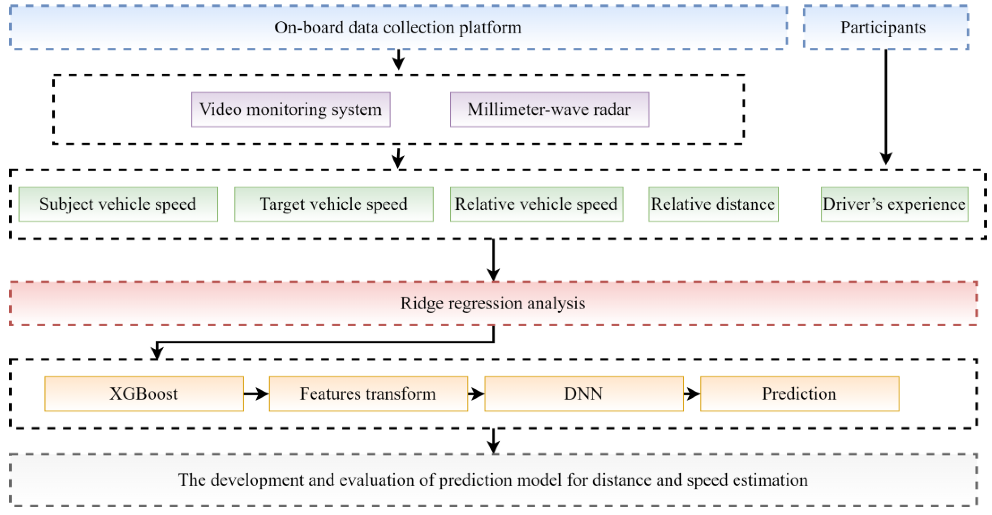
The research framework of this paper is shown in Figure 1, and it is organized as follows. Section 2 introduces the algorithms used to model the speed estimation and distance estimation. Section 3 presents the experiment and elaborates on the data sources for this study. The factors that affect the accuracy of driver speed estimation and distance estimation are analyzed in Section 4. In Section 5, the modeling process of XGBoost-DNN is shown, and the prediction performance of extreme gradient boosting (XGBoost) combined with deep neural network (DNN) algorithms proposed in this paper is compared with that of traditional machine learning algorithms. Section 6 discusses the results. Section 7 concludes the study and provides insights into future work.

2. Description of Algorithms

In this section, we first introduce the XGBoost ensemble learning algorithm and the DNN algorithm separately, and then we describe the mixed algorithm model proposed by combining the XGBoost algorithm and the DNN algorithm innovatively in this paper.

2.1. Description of XGBoost Algorithm

XGBoost, an ensemble learning algorithm, was proposed by Chen and Guestrin [28], and it is essentially an optimized implementation of GBDT [29], which sequentially generates and updates basic classifiers (weakly learned classifiers) to form integrated classifiers (strong classifiers) [30,31]. XGBoost has many advantages. First, XGBoost supports linear classifiers and enables both logistic regression and linear regression. Second, it performs a second-order Taylor expansion of the cost function, enabling the use of second-order derivatives when performing optimization. Third, XGBoost borrows from the RF algorithm and supports column sampling, which reduces computational effort while preventing overfitting [32].

XGBoost is commonly used in the fields of classification and regression, and in recent years, it has been widely noticed for its performance in efficiency and high prediction accuracy [33]. The model structure of XGBoost is shown in Figure 2 and the details of the model can be expressed as follows.

$${\stackrel{⌢}{y}}_i={\displaystyle \sum _{k=1}^K{f}_k(x_i),f_k}\in F$$

(1)

Here, ${\stackrel{⌢}{y}}_i$ is the prediction result of the sample $i$, and $f_k$ is a regression tree; $F$ corresponds to the set of all regression trees; $f_k(x_i)$ represents the calculated score of the $k$-th tree for the $i$-th sample in the data set.

The objective function can be expressed as follows.

$$Obj={\displaystyle \sum _{i=1}^{n}l(y_i,{\stackrel{⌢}{y}}_i)}+{\displaystyle \sum _{k=1}^K\mathsf{\Omega }(f_k)}$$

(2)

$$\mathsf{\Omega }(f_k)=\gamma T+\frac{1}{2}\lambda {\displaystyle \sum _{j=1}^T{w}_j^2}$$

(3)

The loss function of the model is $l(y_i,{\stackrel{⌢}{y}}_i)$, and ${\displaystyle \sum _{k=1}^K\mathsf{\Omega }(f_k)}$. is the regularization term. $\gamma$ and $\lambda$ denote the penalty coefficients on the model; $T$ and $w$ denote the number of leaves and the weights of the leaves of the $k$-th tree, respectively. By splitting the regularization direction into the first $t-1$ and the $t$-th iterations, the loss function becomes the following.

$$Ob{j}^t={\displaystyle \sum _{i=1}^{n}l(y_i,{\stackrel{⌢}{y}}_i^{(t-1)}+f_t(x_i))+\mathsf{\Omega }(f_t)+c}$$

(4)

The new function becomes $f_t(x_i)$ and $c$ is a constant. Subjecting the objective function to a Taylor second-order expansion, we obtain the following.

$$g_i={\partial }_{{\stackrel{⌢}{y}}^{(t-1)}}l(y_i,{\stackrel{⌢}{y}}_i^{(t-1)})$$

(5)

$$h_i={\partial }_{{\stackrel{⌢}{y}}^{(t-1)}}^{2}l(y_i,{\stackrel{⌢}{y}}_i^{(t-1)})$$

(6)

where $g_i$ and $h_i$ are, respectively, the first and second order derivatives of the loss function; thus, the objective function becomes the following.

$$Ob{j}^t={\displaystyle \sum _{i=1}^{n}l(y_i,{\stackrel{⌢}{y}}_i^{(t-1)}+g_i{f}_t(x_i)+\frac{1}{2}{h}_i{f}_t^2(x_i))+\mathsf{\Omega }(f_t)+c}$$

(7)

By removing the constant term, this can be simplified into the following.

$${Obj}^t={\displaystyle \sum _{i=1}^n(g_i{f}_t(x_i)+\frac{1}{2}{h}_i{f}_t^2(x_i))+\mathsf{\Omega }(f_t)}$$

(8)

After transformation and merging the canonical terms, the objective function of the model is described as follows:

$${Obj}^t={\displaystyle \sum _{i=1}^T[({\displaystyle \sum _{i\in I_j}{g}_i})w_j+\frac{1}{2}({\displaystyle \sum _{i\in I_j}{h}_i}+\lambda )w_j^2)+\gamma T}$$

(9)

where $I_j$ is the index number of the instance that falls on the $j$-th leaf node.

2.2. Description of DNN Model

DNN (Deep Neural Network) is a topic of interest in the field of machine learning. DNN model information is stored in the neurons in the network, which has strong robustness and fault tolerance [34]. In addition, DNN has a strong ability to synthesize information and can coordinate well between multiple input information, which is suitable for fusing multiple features of inputs [35]. The internal neural network layers of DNN can be divided into three categories: input layer, hidden layer, and output layer, as shown in Figure 3. The first layer is the input layer, the last layer is the output layer, and the middle layers are all hidden layers. The layers are fully connected to each other, and any neuron in the first layer must be connected to any neuron in the second layer. The correspondence between the input and output values of neurons is as follows:

$$y_i=f(b_j+{\displaystyle \sum _{i=1}^n(x_i\times w_{ij})})$$

(10)

where $x_i$ is the input value, $y_i$ is the output value, $w_{ij}$ is the connection weight, and $b_j$ is the bias value. The role of the activation function is to de-linearize and achieve a nonlinear classification task. In this paper, we introduce the DNN model using the Relu activation function, and the relation can be expressed as follows.

$$f(\delta )=\{\begin{array}{c}\delta ,(\delta \ge 0)\\ 0,(\delta <0)\end{array}$$

(11)

2.3. XGBoost-DNN Mixed Algorithm Model

In this section, we propose a mixed model structure of XGBoost model and DNN model in tandem (Figure 4), where the XGBoost model completes the feature transformation, and finally the DNN model is trained using the fused features, and the DNN model completes the final prediction. The general idea of the proposed model can be described as follows: First, the XGBoost model is trained with existing features; then, the tree learned by the XGBoost model is used to construct new features, and finally these new features are added to the original features to train the DNN model together. The new feature vector is constructed by taking values of 0 and 1, and each element of the vector corresponds to a leaf node of the tree in the XGBoost model. The length of the new feature vector is equal to the sum of the number of leaf nodes in all trees in the XGBoost model.

3. Study Implementation

3.1. Participants

A total of 14 participants (2 females and 12 males) volunteered in the experiment, with ages ranging from 27 to 48 years (mean = 34.7 years) and having 3 to 23 years (mean = 8.4 years) of driving experience. Seven experienced drivers (>5 years of driving experience) and seven non-experienced drivers (<5 years of driving experience) were included. The details of the participants’ information are described in

Table 1. Description of participants’ details.

Participant ID	Gender	Age	Driving Experience
01	male	29	4
02	male	29	4
03	male	28	3
04	male	27	3
05	male	28	4
06	male	48	21
07	male	34	7
08	male	36	10
09	female	42	15
10	male	38	8
11	male	36	7
12	male	48	23
13	female	31	4
14	male	32	5

. All participants had a valid driving license and had not experienced a major traffic accident in the past three years. Participants were prohibited from taking drugs and functional drinks the day before the trial. All were in good health on the day of the trial, and there were no traffic risks during the trial. Each participant willingly volunteered to engage in the experiment, which was approved by the Ethics Committee of Chang’an University. Each participant was given CNY 500 after the trial as compensation for their time.

3.2. Apparatus and Experimental Route

A multifunctional test platform combining a common vehicle and multiple data acquisition devices was deployed for this experiment, and the components of the multifunctional test platform are shown in Figure 5. The millimeter-wave radar was mounted on the center of the rear bumper of the subject vehicle to capture the relative position and relative vehicle speed data between the target vehicle and the subject vehicle. The video monitoring system was used to record the movement of the target vehicle; the GPS was used to record the geographic location of the subject vehicle; the CAN acquisition card obtained the speed information of the subject vehicle; and the wireless button recorded the moment while the participant was performing the task for subsequent data calibration. An industrial control computer was used to collect the data acquired by all components.

In this study, participants were required to look into the rearview mirror several times to estimate the speed and distance of the target vehicle, which may cause distractions while driving. To ensure the safety of the participants, the Xi’an roundabout highway was chosen as the experimental road, where the traffic volume is relatively light, with a two-way six-lane road and having a speed limit of 120 km/h. The total length of the experimental route is 135 km.

3.3. Experimental Design and Procedure

The ability of a driver to decide to change lane depends on an accurate estimation of the speed and distance of the target vehicle. To investigate such an ability, this study conducted realistic road tests at different vehicle speeds. Considering that the daily driving speed for commuters in China mainly ranges from 60 km/h to 90 km/h, we chose 60 km/h, 70 km/h, 80 km/h, and 90 km/h as test speeds. Considering that CCS (Cruise Control System) is becoming more and more common and is increasingly used on highways, in this study, it was simultaneously used to reduce the driver’s workload during driving and to control the longitudinal speed of the subject vehicle. The subject vehicle was required to drive in the middle lane during the test, while the target lane was the left lane (as shown in Figure 6). The target vehicle at the closest distance to the self-vehicle has the greatest influence on the lane change decision during the lane change process, and the driver obtains information about this vehicle through the rearview mirror in daily driving. Therefore, during the test, we requested the driver to estimate the speed and relative distance between the target vehicle and the subject vehicle by using the left rearview mirror.

Before the experiment, the participants were asked to sign an informed consent form and to fill out the basic personal information form. All volunteers were provided a brief description of the trial’s procedure and underwent training on speed and distance estimation tasks, and the formal trial started after the participants were able to complete secondary tasks proficiently.

During the experiment, participants were asked to estimate the speed of the target vehicle and the relative distance to the subject vehicle by using the rearview mirror as many times as possible, verbally report their estimations, and simultaneously press a wireless button mounted on the left side of the steering wheel under the premise of safe driving. In this experiment, an advisor was seated in the rear seat of the subject vehicle and was responsible for monitoring the target vehicle and alerting the participant to make corresponding speed and distance estimations, as well as recording the subject’s verbal report of the results. To ensure driving safety, a veteran driver was always seated in the co-driver’s seat of the subject vehicle to monitor the driving environment and alert the participant if there was a driving risk.

3.4. Variables Definition

In this study, the effects of the speed of the subject vehicle, the speed of the target vehicle, and the relative speed and relative distance between the subject vehicle and the target vehicle on the driver’s speed and distance estimation errors were investigated. Therefore, the analytical variables are the speed of the subject vehicle, the speed of the target vehicle, the relative speed, and the distance. Moreover, the variables are calculated as shown below.

The relative velocity between the subject vehicle and the target vehicle was expressed as follows:

$$V_r=V_s-V_t$$

(12)

where $V_s$ the speed of the subject vehicle $S$, and $V_t$ is the speed of the target vehicle $T$. $V_r$ < 0 indicates that the speed of the subject vehicle $S$ is less than the speed of the target vehicle $T$.

Driver’s speed estimation errors were expressed as follows:

$$V_{er}=V_{es}-V_{re}$$

(13)

where $V_{es}$ is the estimated speed of the target vehicle $T$ from the subject vehicle $S$, and $V_{re}$ is the real speed of the target vehicle $T$. $V_{er}$ < 0 indicates that the driver underestimates the speed of the target vehicle $T$, and $V_{er}$ > 0 indicates that the driver overestimates the speed of the target vehicle $T$.

Driver’s distance estimation errors were evaluated as follows:

$$D_{er}=D_{es}-D_{re}$$

(14)

where $D_{es}$ is the estimated distance between the target vehicle and the subject vehicle, and $D_{re}$ is the real distance between them. $D_{er}$ < 0 indicates that that the driver underestimates the distance between the two vehicles; $D_{er}$ > 0 indicates that that the driver overestimates the distance between the two vehicles.

4. Statistical Analysis Results

Under most lane change circumstances, the speed of the target vehicle T is greater than the speed of the subject vehicle S; therefore, the data for which the speed of vehicle T is less than the speed of vehicle S are excluded. In this study, 2116 sets of relative distance estimation data and 1542 sets of target vehicle speed estimation data were finally collected. Since there were strong linear correlations between the analytical variables, a ridge regression method was used.

Ridge regression, a modified least squares method, is a biased estimation method that is far more accurate than unbiased estimation in the face of the problem of multicollinearity where independent variables are highly correlated [36,37]. There are many methods to set or validate ridge regression parameter $k$, and the most often used is the ridge trace plot, which shows the coefficients as a function of k [38]. The optimal ridge regression coefficient is the minimum $k$ value when the standardized regression coefficients of each independent variable are stabilized as determined by the ridge trace plot.

4.1. Analysis of Relative Distance Estimation Error

4.1.1. General Analysis

The distributions of the motion parameters and distance parameters of the subject vehicle and the target vehicle during the distance estimation are shown in Figure 7. The real distance between the target vehicle and the subject vehicle during the distance estimation fell in the interval [4.23, 186.18], of which about 90% of the distance was clustered between [15.11, 114.90] with a mean value of 56.56 m. The speed of the target vehicle ranged from 52.21 to 174.53 km/h, of which about 60% of the speed of the target vehicle ranged from 95.31 to 119.56 with a mean value of 105.59 km/h. The relative speed of the subject vehicle to the target vehicle fell in the interval [−110.99, −0.04], of which about 75% was clustered in the interval [−49.29, −11.94] with a mean value of −31.66 km/h. The relative distance estimation error fluctuated in the interval [−79.92, 37.38 m], of which about 60% were concentrated in the interval [−12.92, 11.93] with a mean value of −1.15 m.

Among the 2116 valid speed estimation samples collected in the experiment, 1021 samples underestimated the target vehicle, accounting for 48.25% of the total number of samples, and 1095 samples overestimated the target vehicle, accounting for 51.75% of the total number of samples.

4.1.2. Ridge Regression Analysis

The position and speed parameters between the target vehicle and the subject vehicle with distance estimation errors were modeled and analyzed using ridge regression. The ridge trace plots of each parameter coefficient are shown in Figure 8. We found that the coefficients began to stabilize when k = 0.32; thus, 0.32 was chosen as the optimal ridge regression coefficient in this study.

While observing the respective coefficients values (Figure 9), we noticed the following: The regression coefficient value of distance was −0.100 (t = −20.193, p = 0.000 < 0.01), implying that distance has a significant negative incline on its corresponding estimation error; the regression coefficient value of relative vehicle speed was 0.286 (t = 10.775, p = 0.000 < 0.01), implying that relative vehicle speed has a significant positive effect on the distance estimation error; the regression coefficient value of subject vehicle speed km/h was 0.106 (t = 2.240, p = 0.025 < 0.05), implying that the subject vehicle speed has a significant positive bias on the distance estimation error; the regression coefficient value of the target vehicle speed was −0.285 (t = −8.999, p = 0.000 < 0.01), implying that the target vehicle speed has a significant negative effect on the distance estimation error; finally, the regression coefficient value of the driving experience was −0.061 (t = −0.298, p = 0.766 > 0.05), implying that the driving experience does not have a significant impact on the distance estimation error.

In conclusion, it can be seen that the relative speed and subject vehicle speed would have a significant positive influence relationship on the distance estimation error. However, the distance and target vehicle speed would have a significant negative influence on the distance estimation error.

4.2. Analysis of Target Vehicle Speed Estimation Error

4.2.1. General Analysis

The distributions of the motion and distance parameters of the subject and target vehicles during the speed estimation task are shown in Figure 10. The actual distance between the target vehicle and the subject vehicle during the distance estimation fell in the interval [2.16, 196.95], of which about 85% of the distance values were clustered between [9.80, 101.71] with a mean value of 55.73 m. The speed of the target vehicle ranged from 54.17 to 155.29 km/h, of which about 60% of the speed of the target vehicle was between 95.18 and 119.56 with a mean value of 105.27 km/h. The relative speeds of the subject vehicles to the target vehicles varied between −85.35 and −0.03 km/h, of which about 75% fell in the interval [−49.78, −10.94] with a mean value of 31.36 km/h. The speed estimation errors varied in the interval [−41.00, 50.83], of which about 70% of them were concentrated in the interval [−10.73, 16.65], with a mean value of −0.29 km/h.

Among the 1542 valid speed estimation samples collected in the experiment, 804 samples underestimated the target vehicle, accounting for 52.14% of the total number of samples, and 738 samples overestimated the target vehicle, accounting for 47.86% of the total number of samples.

4.2.2. Ridge Regression Analysis

The distance, relative speed, subject vehicle speed, and target vehicle speed were used as independent variables, and speed estimation error was used as dependent variable to perform ridge regression analysis in the process of target vehicle speed estimation. According to the ridge trace plot shown in Figure 11, k = 0.07 was the optimal choice.

The regression coefficients of each analytical variable on the error of speed estimation were shown in Figure 12. The regression coefficient value of distance was −0.040 (t = −5.537, p = 0.000 < 0.01), implying that distance would have a significant negative impact on the speed judgment error. The regression coefficient value of relative speed was 0.185 (t = 20.888, p = 0.000 < 0.01), implying that the relative speed would have a significant positive influence on the speed judgment error. The regression coefficient value of the subject vehicle speed was −0.179 (t = −10.599, p = 0.000 < 0.01), which means that the subject vehicle speed would have a significant negative influence on the speed judgment error. The regression coefficient value of the target vehicle speed was −0.327 (t = −30.224, p = 0.000 < 0.01), implying that the target car speed would have a significant negative incline on the speed judgment error. The regression coefficient value of the driving experience was 0.016 (t = 0.035, p = 0.972 > 0.05), implying that the driving experience would not have a significant influence on the speed judgment error.

Summarizing the analysis, it can be observed that the relative speed will have a significant positive bias on the speed judgment error. However, the distance, subject vehicle speed, and target vehicle speed would have a significant negative influence on the speed judgment error.

5. Modeling of Relative Distance and Velocity Estimation

Based on the factors affecting the driver speed estimation and distance estimation errors selected in the previous section, a prediction model for driver speed estimation and distance estimation based on the integrated learning eXtreme Gradient Boosting (XGBoost) algorithm is developed in this section. Firstly, a coarser two-class prediction model is established; that is, the driver’s estimation results are classified into two categories: overestimation and underestimation. Subsequently, the driver’s estimation results were further subdivided into three categories: overestimation, normal, and underestimation. A more detailed three-classification prediction model is derived.

A total of 1542 sets of speed estimation samples and 2116 sets of distance estimation samples were obtained from the actual road tests. In this paper, the data set was divided into 80% training set and 20% testing set. The input parameters of the model are divided into two categories. One is the driver’s experience; the other is the vehicle motion parameters: subject vehicle speed, target vehicle speed, relative vehicle speed, and relative distance.

5.1. Model Construction

5.1.1. Model Label Settings

To provide a comprehensive overview of the classification performance of the speed and distance estimation model, this paper sets the classification of the speed and distance estimation errors into two cases, namely, two and classifications, according to the specific values of the speed and distance estimation three errors and the distribution of the error values. Specifically, “two classification” is used to classify the driver’s estimation into “overestimation” and “underestimation”. Without a loss of generality, “three classification” is used to classify the driver’s estimation error into “overestimation”, “normal estimation”, and “underestimation”.

In the two-classification of the estimation error, the estimation error value 0 is used as a threshold, when the estimation error is greater than 0, the error value label is set to 1 (overestimation); when the estimation error is less than 0, the error label is set to 0 (underestimation), as shown in Equation (1). In the two-classification model, there are 1020 labels of class 0 and 1096 labels of class 1 in the distance estimation dataset; while in the speed estimation dataset, there are 795 labels of class 0 and 747 labels of class 1.

For tri-classification of estimation errors, the 50% median interval of estimation errors was used as label 2 (normal), the upper 25% interval was used as label 3 (overestimation), and the lower 25% interval was as label 1 (underestimation), as shown in Equations (2) and (3). For the three classifications, there are 519 labels of category 1, 1089 labels of category 2, and 508 labels of category 3 in the distance estimation dataset. In the velocity estimation dataset, there are 374 labels of category 1, 802 labels of category 2, and 366 labels of category 3.

$$E_{2-classs}^{speed-estimate}=\{\begin{array}{c}0,(V_{er}<0)\\ 1,(V_{er}\ge 0)\end{array}$$

(15)

$$E_{2-classs}^{distance-estimate}=\{\begin{array}{c}0,(D_{er}<0)\\ 1,(D_{er}\ge 0)\end{array}$$

(16)

$$E_{3-classs}^{speed-estimate}=\{\begin{array}{c}3,(V_{er}>9)\\ \begin{array}{l}2,(-9\le V_{er}\le 9)\\ 1,(V_{er}<-9)\end{array}\end{array}$$

(17)

$$E_{3-classs}^{distance-estimate}=\{\begin{array}{c}3,(D_{er}>10)\\ \begin{array}{l}2,(-10\le D_{er}\le 10)\\ 1,(D_{er}<-10)\end{array}\end{array}$$

(18)

5.1.2. Model Parameter Settings

In the process of training the prediction model based on XGBoost-DNN algorithm, the parameters were adjusted to achieve the best prediction performance. In the XGBoost model, the key parameters include the learning rate, the number of decision trees, and the maximum depth of the decision trees in which the learning rate can control the step length of updating weights in each iteration of training. The maximum depth of the tree can affect the overfitting phenomenon: The smaller the value, the slower the model training speed is and the easier the model is underfitted, while the larger the value, the easier the model is overfitted.

The main parameters of DNN models include the number of hidden layers and the number of neurons per layer, learning rate, activation function, and optimizer. The deeper the number of layers, the stronger the theoretical performance of the model, but it is prone to overfitting, and too many neurons will also result in overfitting. The learning rate affects the model loss function and changes the convergence rate of the model; the role of the activation function is used to incorporate nonlinear factors to solve problems that cannot be solved by a general linear model; and the role of the optimizer is to update and calculate the model network parameters to approximate or reach the optimal value.

In this paper, the model prediction accuracy is the main criterion to measure the parameter selection. In this paper, we start by determining the value range of each parameter, and then we use iterative calculation and control variables to obtain the value for each parameter that maximizes the model’s prediction accuracy. The specific parameter values are shown in

Table 2. Hyperparameters tuning for XGBoost-DNN in this study.

Class		Hyperparameter	Search Range	Model	Optimal Value
2-class	XGBoost	Learning rate	[0.01, 0.5]	Speed	0.08
				Distance	0.07
		Max tree depth	[2, 10]	Speed	5
				Distance	4
		Minimum loss reduction	[0, 5]	Speed	0
				Distance	0
		Number of estimators	[20, 150]	Speed	55
				Distance	64
	DNN	Hidden layer sizes		Speed	(100,)
				Distance	(100)
		Learning rate	[0.001, 0.1]	Speed	0.001
				Distance	0.001
		Activation	Relu, tanh, Logistic	Speed	Relu
				Distance	Relu
		Solver	SGD, Adam	Speed	SGD
				Distance	SGD
		Number of iterations		Speed	200
				Distance	200
		Batchsize		Speed	Auto
				Distance	Auto
3-class	XGBoost	Learning rate	[0.01, 0.5]	Speed	0.05
				Distance	0.05
		Max tree depth	[2, 10]	Speed	6
				Distance	6
		Minimum loss reduction	[0, 5]	Speed	0
				Distance	0
		Number of estimator	[20, 150]	Speed	67
				Distance	73
	DNN	Hidden layer sizes		Speed	(100)
				Distance	(100)
		Learning rate	[0.001, 0.1]	Speed	0.001
				Distance	0.001
		Activation	Relu, tanh, Logistic	Speed	Relu
				Distance	Relu
		Solver	SGD, Adam	Speed	SGD
				Distance	SGD
		Number of iterations		Speed	200
				Distance	200
		Batchsize		Speed	Auto
				Distance	Auto

.

In this paper, we use the Python-Sklearn package to train the model with an Intel i9-12900 K CPU and 64 GB of running memory. In the DNN module, the parameter tol is the condition for the model to stop training, and we set tol to 0.001, which means the model stops training when the loss value is less than or equal to 0.001. To avoid overfitting, we adjust the parameter’s subsample and colsample-bytree in the XGBoost module, which represent the ratio of the data and features used in training each tree to the total training set and features, respectively, with typical values of 0.5–1. By adjusting these two parameters, the overfitting of the model can be prevented.

5.2. Model Evaluation

5.2.1. Model Evaluation Methods

Confusion matrices with good visualization are often used to evaluate the performance of machine learning models [39,40,41]. In this paper, the confusion matrix is used to evaluate the performance of the binary prediction model and the triple classification prediction model. For k-element classification, the confusion matrix is represented as a matrix of size k × k. As an example, the binary confusion matrix is described in Table 2. True Positive (TP), False Negative (FN), True Negative (TN), and False Positive (FP) are the main indicators of the confusion matrix, and the substantial meaning of each indicator is shown in

Table 3. Description of the actual meaning of confusion matrix.

Confusion matrix		Predicted values (Model prediction outcome)
		Overestimation (Positive)	Underestimation (Negative)
True values (Driver’s estimation outcome)	Overestimation (Positive)	True Positive (TP)	False Negative (FN)
	Underestimation (Negative)	False Positive (FP)	True Negative (TN)

.

The metrics accuracy rate ($Acc$), precision rate ($P$), recall rate ($R$), and $F_1$-score (F1), which are commonly used for classification model evaluation, can be calculated using these metrics [42]. The formula for each metric is shown below.

$$Acc=\frac{TP+TN}{TP+TN+FP+FN}$$

(19)

$$P=\frac{TP}{TP+FP}$$

(20)

$$R=\frac{TP}{TP+FN}$$

(21)

$$F_1=\frac{2PR}{P+R}$$

(22)

The Receiver Operating Characteristic (ROC) curve is also used to measure the training performance of the model. The ROC curve shows the probability of TP rate and FP rate under different threshold settings, while the Area Under Curve (AUC), which is the region under the ROC curve, reveals better classification performance when its value ranges from 0.5 to 1. The ROC curve is more suitable for evaluating the binary prediction problem; therefore, when evaluating the latter, it is used in addition to the confusion matrix.

5.2.2. Model Evaluation Results

Without loss of generality, in order to verify the applicability of the prediction model based on the XGBoost-DNN mixed algorithm for predicting the driver’s lane change speed and distance estimation, this paper compared its performance with traditional machine algorithm models such as Logistic Regression (LR) [43], Random Forest (RF) [44], Support Vector Machine (SVM) [45,46], K-Nearest Neighbor (KNN) [47], Deep Neural Networks (DNN) [34,35], Gradient Boosting Decision Tree (GBDT) [48], and XGBoost models [49].

Table 4. Model evaluation results for different algorithms (two-classification).

Algorithm	Speed Estimation				Distance Estimation
	Acc (%)	P	R	F1	Acc (%)	P	R	F1
RF	75.32	75.38	74.90	75.01	78.83	81.32	78.44	78.23
SVM	69.23	69.07	68.94	68.98	68.37	69.08	68.07	67.83
LR	73.08	72.96	73.03	72.99	68.37	68.34	68.32	68.32
KNN	76.92	76.89	76.62	76.71	73.23	73.78	73.01	72.94
DNN	75.96	76.85	76.55	75.94	72.26	72.42	72.36	72.25
GDBT	85.58	85.64	85.35	85.45	86.62	86.64	86.58	86.60
XGBoost	88.78	88.83	88.61	88.70	90.51	90.54	90.47	90.50
XGBoost-DNN	91.03	91.02	90.94	90.72	92.46	92.45	92.48	92.46

reports the results of the two-classification model evaluation for speed estimation and distance estimation, and it was found that the model’s accuracy reaches 91.03% in speed estimation and 92.46% in distance estimation.

It can be observed from Table 4 that XGBoost-DNN has the highest recognition accuracy of 91.03% in speed estimation, which is about 22% greater than the accuracy of SVM model. Compared with RF, LR, KNN, and GBDT models, XGBoost-DNN showed considerable advantages. In addition, the recognition accuracy of XGBoost-DNN is about 2.25% higher than that of the XGBoost model. Similar results are found in distance estimation, and the recognition accuracy of XGBoost-DNN is also the highest, reaching 92.46%, which is about 24% higher than that of the SVM model. Moreover, the recognition accuracy of XGBoost-DNN is about 1.91% higher than that of XGBoost model.

Figure 13 depicts the values of model evaluation metrics for speed estimation and distance estimation for the two-classification case for different models. It is apparent from Figure 13 that the XGBoost-DNN proposed in this paper outperforms the other seven models. Moreover, the prediction performance of XGBoost is ranked second among the seven prediction models.

Figure 14 depicts that the AUC values of the XGBoost-DNN speed estimation model and distance estimation model are 0.957 and 0.963, respectively, which are higher than those obtained using traditional machine learning models. This indicates that the ROC curves also support the observation that the XGBoost-DNN model has better performance in the two-classification cases.

Table 5. Model evaluation results for different algorithms (three-classification).

Algorithm	Speed Estimation				Distance Estimation
	Acc (%)	P	R	F1	Acc (%)	P	R	F1
RF	68.27	75.33	57.08	59.94	65.21	74.56	58.83	56.55
SVM	63.78	68.26	51.32	53.21	51.82	36.42	41.88	36.64
LR	63.46	62.31	56.32	58.24	55.72	60.28	49.08	47.89
KNN	63.46	62.51	56.87	58.61	62.77	65.02	57.09	57.66
DNN	65.06	67.40	55.93	58.85	61.31	64.51	57.49	56.62
GDBT	80.13	79.72	78.00	78.78	78.10	80.10	75.49	76.97
XGBoost	85.25	84.66	84.42	84.44	86.62	87.76	85.07	86.03
XGBoost-DNN	87.18	88.05	85.05	86.39	87.59	87.85	87.00	87.38

reports the results of the three-classification model evaluation for speed estimation and distance estimation, and it was found that the model accuracy reaches 87.18% in speed estimation and 87.59% in distance estimation.

Figure 15 depicts the values of model evaluation metrics for speed estimation and distance estimation for the three-classification case for different models. It is apparent from Figure 15 that the XGBoost-DNN proposed in this paper outperforms the other seven models. Moreover, the prediction performance of XGBoost is ranked second among the seven prediction models.

In summary, for the two-classification problem, high performance is achieved by all three models where the accuracy of all three models is above 72%. However, the XGBoost-DNN model has the highest prediction accuracy, with, respectively, 91.03% and 92.46% for speed and distance estimations, which is much higher than traditional machine learning models, proving excellent prediction accuracy. When compared to the two-classification prediction models, the performances of the three-classification prediction models built using the traditional machine learning algorithms and the XGBoost-DNN mixed algorithm proposed in this paper all plummeted. However, the XBoost-DNN model showed the lowest drop in performance. For speed and distance estimations, the accuracy is 87.18% and 87.59%, respectively, and the prediction accuracy is still better compared to the other traditional machine learning models.

6. Discussion

The risk assessment in driver lane changing mainly comes from the assessment of relative speed and relative distance between the target vehicle and the subject’s own vehicle, and the results of driver assessments are directly related to traffic risk and traffic efficiency. However, in the current lane-change research area, few researchers have conducted studies on the speed and distance estimation of drivers by using the rearview mirror during the lane-changing decision process. For this reason, in this study, an actual live highway test was conducted, during which the participants were asked to turn on CCS and make sequential estimates of the absolute speed of the target vehicle and the distance from the subject vehicle at four speeds controlled by CCS: 60, 70, 80, and 90 km/h. Firstly, we explored the surrounding factors that affect driver’s speed estimation and distance estimation errors. Subsequently, two- and three-classification prediction models for driver speed estimation and distance estimation results were developed based on the XGBoost-DNN mixed algorithm.

The results of the ridge regression showed that, in the speed and distance estimations, the speed of the subject vehicle, the speed of the target vehicle, the relative speed, and the relative distance between the subject vehicle and the target vehicle all had significant impact on the estimation error. The larger the relative speed and target vehicle speed, the more the driver tends to underestimate the speed and distance of the target vehicle. The smaller the relative speed and target speed, the more the driver tends to overestimate the speed and distance of the target vehicle. In addition, it can be observed in speed estimation that the higher the speed of the subject vehicle, the more the driver tends to underestimate the speed of the target vehicle; the lower the speed of the subject vehicle, the more the driver tends to overestimate the speed of the target vehicle. However, in distance estimation, the lower the speed of the subject vehicle, the more the driver tended to underestimate the relative distance; the higher the speed of the subject vehicle, the more the driver tended to overestimate the relative distance. In this study, we did not find a conclusive effect of driving experience on speed estimation error and distance estimation error. In addition, it can be observed from the coefficients of the variables in the ridge regression model that both the target vehicle speed and the relative vehicle speed have a large effect on the errors in speed estimation and distance estimation. This study on the effect of test and target vehicle speeds on driver estimation error is consistent with the findings by Wang, et al. [50].

In this study, a driver speed estimation and distance estimation model based on XGBoost-DNN mixed algorithm was established. In the two-classification models, we classify drivers into two categories based on their estimation errors with respect to zero: underestimation and overestimation. The prediction accuracy of the XGBoost-DNN algorithm-based binary classification model for speed estimation and distance estimation reached 91.03% and 92.46%, respectively, which is about two percentage points higher than that of the XGBoost algorithm. Both the confusion matrix method and the ROC curve method proved that the prediction model based on XGBoost-DNN for the two-classification estimation outperformed other traditional machine learning models. In the three-classification model, drivers in the data sample were classified into three categories according to their estimation error distribution: underestimation, normal, and overestimation. The prediction accuracy of the three-classification model based on XGBoost-DNN algorithm reached 87.18% and 87.59% for speed estimation and distance estimation, respectively. The performance of the XGBoost-DNN algorithm-based dichotomous estimation prediction model was verified to be better than that of traditional machine learning models by the confusion matrix method.

Although the prediction accuracy of the XGBoost-DNN algorithm-based driver speed estimation and distance estimation three-classification prediction model is lower than that of the two-classification model, its classification is more specific and can predict the driver’s estimation error situation more accurately.

7. Conclusions and Future Work

In this study, we found that environmental factors affect drivers’ estimation results. The greater the relative speed and target vehicle speed, the more drivers tend to underestimate the speed and distance of the target vehicle. Therefore, drivers should be reminded to focus extra attention to lane-change safety in such cases. We suggest that driver training efforts can be carried out to train drivers to correctly estimate the target vehicle. The XGBoost-DNN model has a better prediction of driver estimation, which is helpful for providing a theoretical basis for a smarter warning rule for driver lane change warning systems.

In order to further improve the intelligence of the lane change warning system, we will continue to extend this research work in the future. Firstly, we will conduct larger scale trials on real roads to obtain more participants’ environmental estimation data. Secondly, we will recruit more types of participants (e.g., more age and driving experience coverage) in future trials, and we will try to achieve gender balance in the participants. Finally, the driver’s lane change process can be divided into three stages: information perception, lane change decision, and action execution. In this study, we explore the process of information perception, and we will gradually explore the other two stages in our future research.

References

1. Liu, X.; Jin, G.; Wang, Y.; Yin, C. A Deep Learning-based Approach to Line Crossing Prediction for Lane Change Maneuver of Adjacent Target Vehicles. In Proceedings of the 2021 IEEE International Conference on Mechatronics (ICM), Kashiwa, Japan, 7–9 March 2021; pp. 1–6. [Google Scholar]
2. Sun, D.; Elefteriadou, L. Lane-Changing Behavior on Urban Streets: An “In-Vehicle” Field Experiment-Based Study. Comput.-Aided Civ. Infrastruct. Eng. 2012, 27, 525–542. [Google Scholar] [CrossRef]
3. Wang, J.R.K. IVHS/Crash Avoidance Countermeasure Targe. In Proceedings of the Safety & Human Factors Session of 1993 IVHS America Annual Meeting, Santa Monica, CA, USA, 14–17 April 1993. [Google Scholar]
4. Risto, M.; Martens, M.H. Driver headway choice: A comparison between driving simulator and real-road driving. Transp. Res. Part F Traffic Psychol. Behav. 2014, 25, 1–9. [Google Scholar] [CrossRef]
5. Eberhard, C.D.; Luebkemann, K.M.; Moffa, P.J.; Young, S.K.; Allen, R.W.; Harwin, E.A.; Keating, J.; Mason, R. Development Of Performance Specifications for Collision Avoidance Systems for Lane Change, Merging and Backing, Task 1—Interim Report: Crash Problem Analysis; National Highway Traffic Safety Administration: Washington, DC, USA, 1995.
6. Shawky, M. Factors affecting lane change crashes. IATSS Res. 2020, 44, 155–161. [Google Scholar] [CrossRef]
7. Peng, J.; Guo, Y.; Fu, R.; Yuan, W.; Wang, C. Multi-parameter prediction of drivers’ lane-changing behaviour with neural network model. Appl. Ergon. 2015, 50, 207–217. [Google Scholar] [CrossRef]
8. Yan, F.; Eilers, M.; Baumann, M.; Luedtke, A. Development of a Lane Change Assistance System Adapting to Driver’s Uncertainty During Decision-Making. In Proceedings of the Adjunct 8th International Conference on Automotive User Interfaces and Interactive Vehicular Applications, Ann Arbor, MI, USA, 24–26 October 2016; pp. 93–98. [Google Scholar]
9. Milanés, V.; Alonso, J.; Bouraoui, L.; Ploeg, J. Cooperative Maneuvering in Close Environments Among Cybercars and Dual-Mode Cars. IEEE Trans. Intell. Transp. Syst. 2011, 12, 15–24. [Google Scholar] [CrossRef] [Green Version]
10. Wang, C.; Sun, Q.; Guo, Y.; Fu, R.; Yuan, W. Improving the User Acceptability of Advanced Driver Assistance Systems Based on Different Driving Styles: A Case Study of Lane Change Warning Systems. IEEE Trans. Intell. Transp. Syst. 2020, 21, 4196–4208. [Google Scholar] [CrossRef]
11. Chen, C.; Lü, N.; Liu, L.; Pei, Q.-Q.; Li, X.-J. Critical safe distance design to improve driving safety based on vehicle-to-vehicle communications. J. Cent. South Univ. 2013, 20, 3334–3344. [Google Scholar] [CrossRef]
12. Hidas, P. Modelling lane changing and merging in microscopic traffic simulation. Transp. Res. Part C Emerg. Technol. 2002, 10, 351–371. [Google Scholar] [CrossRef]
13. Qiu, T. Research on Learning Based Lane Keeping and Lane Changing Behaviors of Intelligent Vehicle. Master’s Thesis, Beijing University of Technology, Beijing, China, 2019. [Google Scholar]
14. Xu, B.; Liu, X.; Wang, Z.; Liu, F.; Liang, J. Fusion decision model for vehicle lane change with Fusion decision model for vehicle lane change with. J. Zhejiang Univ. 2019, 53, 1171–1181. [Google Scholar] [CrossRef]
15. Shi, C. Analysis of Driving Suitability of Novice Drivers. China Saf. Sci. J. 2013, 23, 20–26. [Google Scholar] [CrossRef]
16. Shi, C.; Ou, J.; Cao, J. Analysis of psychological and physiological characteristics of people with bad driving behavior. Chin. J. Ergon. 2013, 19, 56–59. [Google Scholar] [CrossRef]
17. Snowden, R.J.; Stimpson, N.; Ruddle, R.A. Speed perception fogs up as visibility drops. Nature 1998, 392, 450. [Google Scholar] [CrossRef] [PubMed]
18. Sokolov, A.N.; Ehrenstein, W.H.; Pavlova, M.A.; Cavonius, C.R. Motion Extrapolation and Velocity Transposition. Perception 1997, 26, 875–889. [Google Scholar] [CrossRef] [PubMed]
19. DeLucia, P.R. Effects of Size on Collision Perception and Implications for Perceptual Theory and Transportation Safety. Curr. Dir. Psychol. Sci. 2013, 22, 199–204. [Google Scholar] [CrossRef]
20. Wu, C.; Yu, D.; Doherty, A.; Zhang, T.; Kust, L.; Luo, G. An investigation of perceived vehicle speed from a driver’s perspective. PLoS ONE 2017, 12, e0185347. [Google Scholar] [CrossRef] [PubMed] [Green Version]
21. Sun, R.; Zhuang, X.; Wu, C.; Zhao, G.; Zhang, K. The estimation of vehicle speed and stopping distance by pedestrians crossing streets in a naturalistic traffic environment. Transp. Res. Part F Traffic Psychol. Behav. 2015, 30, 97–106. [Google Scholar] [CrossRef]
22. Yan, B.; Chen, H.; Wei, J. Influence of Drivers’ Perceptual Features on Traffic Safety in Tunnel Group. China Saf. Sci. J. 2011, 21, 16–21. [Google Scholar] [CrossRef]
23. Peng, J. Drivers Lane Change Intent Identification Based on Visual Characteristics and Vehicles’ Relative Movements. Ph.D. Thesis, Changan University, Xian, China, 2012. [Google Scholar]
24. Haglund, M.; Åberg, L. Speed choice in relation to speed limit and influences from other drivers. Transp. Res. Part F Traffic Psychol. Behav. 2000, 3, 39–51. [Google Scholar] [CrossRef]
25. Michaels, R.M. Perceptual Factors in Car-Following. In Proceedings of the 2nd International Symposium on the Theory of Road Traffic Flow, London, UK, 25–27 June 1963; pp. 44–59. [Google Scholar]
26. Kang, G. The Study of Driver’s Space Distance Judgment on Ground Dynamic Environment. Master’s Thesis, Changan University, Xian, China, 2005. [Google Scholar]
27. Wei, J.; Zhao, W.; Baolin, X. Effects of different factors on visual cognition distance of drivers at night. China Saf. Sci. J. 2013, 23, 21–27. [Google Scholar] [CrossRef]
28. Chen, T.; Guestrin, C. XGBoost: A Scalable Tree Boosting System. In Proceedings of the 22nd ACM SIGKDD International Conference on Knowledge Discovery and Data Mining, San Francisco, CA, USA, 13–17 August 2016; pp. 785–794. [Google Scholar]
29. Xu, Y.; Zhao, X.; Chen, Y.; Yang, Z. Research on a Mixed Gas Classification Algorithm Based on Extreme Random Tree. Appl. Sci. 2019, 9, 1728. [Google Scholar] [CrossRef] [Green Version]
30. Wang, K.; Xue, Q.; Xing, Y.; Li, C. Improve Aggressive Driver Recognition Using Collision Surrogate Measurement and Imbalanced Class Boosting. J. Environ. Res. Public Health 2020, 17, 2375. [Google Scholar] [CrossRef] [PubMed] [Green Version]
31. Wang, X.; Wang, L.; Wang, S.; Chen, J.-F.; Wu, C. An XGBoost-enhanced fast constructive algorithm for food delivery route planning problem. Comput. Ind. Eng. 2021, 152, 107029. [Google Scholar] [CrossRef]
32. Krizhevsky, A.; Sutskever, I.; Hinton, G.E. ImageNet classification with deep convolutional neural networks. In Proceedings of the 25th International Conference on Neural Information Processing Systems, Lake Tahoe, NV, USA, 3–6 December 2012; Volume 1, pp. 1097–1105. [Google Scholar]
33. Song, K.; Yan, F.; Ding, T.; Gao, L.; Lu, S. A steel property optimization model based on the XGBoost algorithm and improved PSO. Comput. Mater. Sci. 2020, 174, 109472. [Google Scholar] [CrossRef]
34. Toshev, A.; Szegedy, C. DeepPose: Human Pose Estimation via Deep Neural Networks. In Proceedings of the 27th IEEE Conference on Computer Vision and Pattern Recognition (CVPR), Columbus, OH, USA, 23–28 June 2014; pp. 1653–1660. [Google Scholar]
35. Wang, S.H.; Mo, B.C.; Zhao, J.H. Deep neural networks for choice analysis: Architecture design with alternative-specific utility functions. Transp. Res. Part C-Emerg. Technol. 2020, 112, 234–251. [Google Scholar] [CrossRef]
36. Hoerl, A.E.; Kennard, R.W. Ridge regression: Biased estimation for nonorthogonal problems. Technometrics 2000, 42, 80–86. [Google Scholar] [CrossRef]
37. Whittaker, J.C.; Thompson, R.; Denham, M.C. Marker-assisted selection using ridge regression. Genet. Res. 2000, 75, 249–252. [Google Scholar] [CrossRef]
38. Zhang, R.; McDonald, G.C. Characterization of ridge trace behavior. Commun. Stat.-Theory Methods 2005, 34, 1487–1501. [Google Scholar] [CrossRef]
39. Fawcett, T. An introduction to ROC analysis. Pattern Recognit. Lett. 2006, 27, 861–874. [Google Scholar] [CrossRef]
40. Stehman, S.V. Selecting and interpreting measures of thematic classification accuracy. Remote Sens. Environ. 1997, 62, 77–89. [Google Scholar] [CrossRef]
41. Tharwat, A. Classification assessment methods. Appl. Comput. Inform. 2021, 17, 168–192. [Google Scholar] [CrossRef]
42. Zhang, H.; Guo, Y.; Wang, C.; Fu, R. Stacking-based ensemble learning method for the recognition of the preceding vehicle lane-changing manoeuvre: A naturalistic driving study on the highway. IET Intell. Transp. Syst. 2022, 16, 489–503. [Google Scholar] [CrossRef]
43. Nwadiuto, J.C.; Yoshino, S.; Okuda, H.; Suzuki, T. Variable Selection and Modeling of Drivers’ Decision in Overtaking Behavior Based on Logistic Regression Model With Gazing Information. IEEE Access 2021, 9, 127672–127684. [Google Scholar] [CrossRef]
44. Ding, J.; Bar-Joseph, Z. MethRaFo: MeDIP-seq methylation estimate using a Random Forest Regressor. Bioinformatics 2017, 33, 3477–3479. [Google Scholar] [CrossRef] [PubMed]
45. Yang, X.; Yu, Q.; He, L.; Guo, T. The one-against-all partition based binary tree support vector machine algorithms for multi-class classification. Neurocomputing 2013, 113, 1–7. [Google Scholar] [CrossRef]
46. Madzarov, G.; Gjorgjevikj, D.; Chorbev, I. A Multi-class SVM Classifier Utilizing Binary Decision Tree. Informatica 2009, 33, 225–233. [Google Scholar] [CrossRef]
47. Zhou, R.S.; Wang, Z.J. A Review of a Text Classification Technique: K-Nearest Neighbor. In Proceedings of the International Conference on Computer Information Systems and Industrial Applications (CISIA), Bangkok, Thailand, 28–29 June 2015; pp. 453–455. [Google Scholar]
48. Ma, X.L.; Ding, C.; Luan, S.; Wang, Y.; Wang, Y.P. Prioritizing Influential Factors for Freeway Incident Clearance Time Prediction Using the Gradient Boosting Decision Trees Method. IEEE Trans. Intell. Transp. Syst. 2017, 18, 2303–2310. [Google Scholar] [CrossRef]
49. Zheng, H.T.; Yuan, J.B.; Chen, L. Short-Term Load Forecasting Using EMD-LSTM Neural Networks with a Xgboost Algorithm for Feature Importance Evaluation. Energies 2017, 10, 1168. [Google Scholar] [CrossRef] [Green Version]
50. Wang, C.; Fu, R.; Zhang, Q. Speed estimation model during lane-changing decision. J. Traffic Transp. Eng. 2015, 16, 83–91. [Google Scholar] [CrossRef]
Figure 1. Research framework.
Sustainability 14 06829 g001
Figure 2. XGBoost structure.
Sustainability 14 06829 g002
Figure 3. DNN structure.
Sustainability 14 06829 g003
Figure 4. XGBoost-DNN mixed model structure.
Sustainability 14 06829 g004
Figure 5. Multifunctional test platform.
Sustainability 14 06829 g005
Figure 6. The experiment of relative distance and speed estimation by the participant driving subject vehicle S to the target vehicle T at the rear of the target lane.
Sustainability 14 06829 g006
Figure 7. Distribution of target vehicle motion and position parameters during relative distance estimation task.
Sustainability 14 06829 g007
Figure 8. Distance estimation task ridge trace plot.
Sustainability 14 06829 g008
Figure 9. The weights of the effects of each analytical variable on the error of distance estimation.
Sustainability 14 06829 g009
Figure 10. Distribution of target vehicle motion and position parameters during relative speed estimation task.
Sustainability 14 06829 g010
Figure 11. Speed estimation task ridge trace plot.
Sustainability 14 06829 g011
Figure 12. The weights of the effects of each analytical variable on the error of speed estimation.
Sustainability 14 06829 g012
Figure 13. Evaluation results of different algorithms in two-classifications. (a) Speed estimation prediction model; (b) distance estimation prediction model.
Sustainability 14 06829 g013
Figure 14. ROC curves of the prediction models. (a) Speed estimation prediction model; (b) distance estimation prediction model.
Sustainability 14 06829 g014
Figure 15. Evaluation results of different algorithms in three-classifications. (a) Speed estimation prediction model; (b) distance estimation prediction model.
Sustainability 14 06829 g015