Using Modified Harmonic Analysis to Estimate the Trend of Sea-Level Rise around Taiwan

Abstract

Sea-level rise (SLR) has become an essential global environmental problem and great importance is attached by all sectors of society. This study aims to estimate the trends of SLR from the tide-gauge measurements located in different sites of Taiwan. Different methods of analysis, such as the linear-regression method (LRM), Hilbert–Huang transform (HHT), and modified harmonic analysis (MHA) are used to estimate SLR and their applicability is discussed. Limitations of these methods are also compared and discussed via the analyzed results. MHA is the focus of the present paper. It has the advantage of representing tidal harmonic motion as well as the long-term trend of SLR more accurately, even in the condition of data loss caused by mechanical failures or anomaly. The analyzing results reveal that MHA is more applicable for estimating SLR than the above traditional methods. The most important analyzed results indicate that the recent 20-year SLR rate is within the range of −0.9 mm/yr and 18.1 mm/yr, using the tidal database observed at 17 stations along the Taiwanese coast. SLR is also compared with analyzed results from different databases or scenarios. The value of SLR is modified by adding the vertical-change rate of the benchmark. It is interesting to note that correction tends to reduce the bias of the variation trend of SLR.

1. Introduction

In the context of global climate change, sea-level rise (SLR) and extreme weather events have become much more severe, leading to the aggravation of various marine and coastal disasters. These disasters also have led to a gradual increase in economic losses. SLR could lead to frequent flooding, flat coasts, storm surges, and saltwater intrusion. Methods to accurately evaluate coastal disasters caused by changes in SLR are crucial for disaster prevention and mitigation around coastal regions. SLR, in the context of global climate change, is considered to be the most severe impact caused by climate change [1,2].

Research on SLR is globally popular, such as [3,4,5,6,7,8,9,10,11,12,13,14,15,16,17,18,19,20,21,22,23,24,25,26,27,28,29,30,31,32,33,34]. The analysis of SLR normally is based on databases or scenarios: (1) measurements from tide gauges at different locations [8,22,23,31,32]; (2) records of satellite altimetry [6,11,13,14,15,22,24,33]; (3) increasing temperatures leading to North and South Pole ice melting [25,27,28,29], and (4) the greenhouse effect and higher CO₂-emissions scenarios [9,10,12,21,23,26].

Merrifield et al. [8] used data from a tidal station for estimating the rate of global SLR. The results are quite consistent with Church and White [6], analyzing the data records of satellite altimetry. Hay et al. [22] combines tide-gauge records with physics-based and model-derived geometries of the various contributing signals to analyzed SLR. The result shows that global SLR grew at a rate of 3.0 ± 0.7 mm/yr from 1993 to 2010. Dangendorf et al. [23] estimates the increasing rate is within the range of 1.1 ± 0.3 mm/yr before 1990, and 3.1 ± 1.4 mm/yr from 1993 to 2012. In the same way, these interesting results are analyzed by performing EMD [31,32].

Nerem et al. [11] used satellite altimetry (SA) data to analyze the SLR changes observed from 1992 to 2014. The report shows that SLR increases an average of 0.3 cm/year. Note that the thermal expansion of the ocean caused by gas warming has a longer hysteresis process. Nicholls and Cazenave [13] used SAD to explore the pattern of SLR along the Chinese Coast. It is found that the SLR rate of the western Pacific Ocean is the most significant. Xu et al. [14] applied the empirical-orthogonal-function (EOF) method to analyze the SLR of the North Pacific, using SA data from 1993 to 2006. Ablain et al. [15] observed the gravity field of the earth through gravity correction and climate experiment (GRACE) and combined the observation results of satellite-altimetry SA and ARGO systems. They found that since 2003, the rise in sea level is mainly due to the increased quality of seawater. Kopp et al. [24] present local SLR projections to make decisions for long-term timescales ranging from the coming decades through the 22nd century. It is interesting to note that SLR rates in various regions of the world are not consistent using SA data. [33].

The IPCC (AR5) points out that the global SLR grows about 0.19 m/yr and has a rising average rate of 1.7mm/yr, 0.28~0.98 m from 1901 to 2010 and the end of the 21st century, respectively. PCC AR6 shows that the mean rate of global SLR is consistent in the latter period. Manabe and Stouffer [12] report that SLR will continue at an equal rate of about 20 mm/yr due to thermal expansion, a total increase of 1 m in 500 years. Global mean SLR has received much attention by many researchers, and their reports point out that SLR has been ranging from 11 cm to 16 cm in the 20th century [21,22,23]. Nauels et al. [26] find that 2100 median SSP on SLR projections could be limited to around 50 cm if 2050 cumulative CO₂ emissions, since the pre-industrial era, stay below 850 GtC. Under higher-emissions scenarios, it is also noted that 21st century SLR may approach or extremely exceed 2 m, in the case of early-onset Antarctic-ice-sheet instability [25,26,27,28]. A global SLR exceeding 2 m by 2100 lies within the 90% uncertainty bounds for a high-emission scenario [29]. Note that this estimate is more than twice the upper value of the IPCC AR5.

2. Methods of Analysis

Harmonic Analysis (HA) is the traditional method for tidal analysis to describe its astronomical tidal components. In practical applications, $k$ sub-tides are selected to obtain the best approximate tidal motion, to get higher accuracy. The governing equation is given by

$$y\left(t^{\prime }\right)=A_0+{\displaystyle \sum }_{r=1}^k{A}_r\cos {\omega }_r{t}^{\prime }+{\displaystyle \sum }_{r=1}^k{B}_r\sin {\omega }_r{t}^{\prime }$$

(1)

where $y\left(t^{\prime }\right)$ is the tide level at a time. Normally, 60 tidal components are used for HA analysis. We use HA to analyze the average sea-level change at different tide stations of Taiwan. Note that the value of $A_0$ is a constant. A different data length will obtain different values of $A_0$. These values at a different period make it confusing to understand the long-term variation of SLR. Therefore, it is difficult to estimate the increasing trend of SLR for long-term temporal variations in science or engineering practice.

In order to remove the confinement for precise estimates of the traditional HA method, we propose a reconciliation analysis of LRM to precisely represent the increase in SLR for a long period. However, LRM is unable to represent the temporal variation of tidal harmonic motion. It is unrealistic for LRM to stand for tidal motion caused by astronomic components.

Huang et al. [16] addresses the Hilbert–Huang transform (HHT), to represent the signals of tide motion by many non-linear components. The Hilbert–Huang transform (HHT) was proposed by Norden E. Huang et al. [16], which is an extension of empirical-mode decomposition (EMD) and the Hilbert transform (HT). The fundamental part of the HHT is the empirical-mode-decomposition (EMD) method. The HHT uses the EMD method to decompose a signal into a so-called intrinsic-mode function (IMF), with a trend. The Hilbert–Huang transform (HHT) is able to decompose a signal into an intrinsic mode function (IMF), along with a trend, and obtain instantaneous frequency data. It is noted that HHT includes empirical-mode decomposition (EMD) and the Hilbert transform (HT). Huang et al. [16,17] used the internal time scale of data variation for an immediate resolution of energy, which expresses the raw data as intrinsic-mode function (IMF) components, in which the IMF has a clear physical meaning, high accuracy, and great orthogonally and adaptability, plus it provides an apparent local detail of the time-frequency characteristics. In HHT, Wu et al. [18] used the ensemble-empirical-mode-decomposition (EEMD) method to decompose actual fluctuations with different scales. However, HHT has the disadvantage of simulating long tide motion for the case of data missing. Huang et al. [17] also pointed out that HHT has an ending swing problem because there is a gap between the first and last data points. Therefore, it is difficult to yield an object-trend-SLR rate. For this reason, this paper proposes an improved harmonic-analysis method to redefine the trend signal. We divide the signal into a periodic signal and a linear-variation trend, i.e., signal = periodic signal + trend (polynomial or linear equation). The periodic signal is in terms of the astronomical tide, and the polynomial or linear equation represents the increasing trend, respectively. The mathematical equation is as follows.

$$\begin{array}{c}h(t)=\underset{\mathrm{periodic}\mathrm{signal}\left(\mathrm{astronomical}\mathrm{tide}\right)}{\underbrace{\left[{\displaystyle \sum _{n=1}^{\infty }{A}_n\cos }{\omega }_{n}t+{\displaystyle \sum _{n=1}^{\infty }{B}_n\sin {\omega }_{n}t}\right]}}+\underset{\mathrm{trend}\mathrm{signal}}{\underbrace{{\displaystyle \sum _{k=0}^m{C}_k{t}^k}}}\\ =\underset{\mathrm{periodic}\mathrm{signal}\left(\mathrm{astronomical}\mathrm{tide}\right)}{\underbrace{{\displaystyle \sum _{n=1}^{\infty }{H}_n\cos ({\omega }_{n}t-{\epsilon }_n)}}}+\underset{\mathrm{trend}\left(\mathrm{SLR}\right)}{\underbrace{{\displaystyle \sum _{k=0}^m{C}_k{t}^k}}}\end{array}$$

(2)

where ${\omega }_n$ is the angular frequency, $H_n$ the amplitude, and ${\epsilon }_n$ the phase lag of the tide components. Note that an expression of polynomial or linearity denotes the trend signal, for representing the amount of SLR. The coefficients in Equation (2) can be obtained by LRM.

3. Results and Discussion

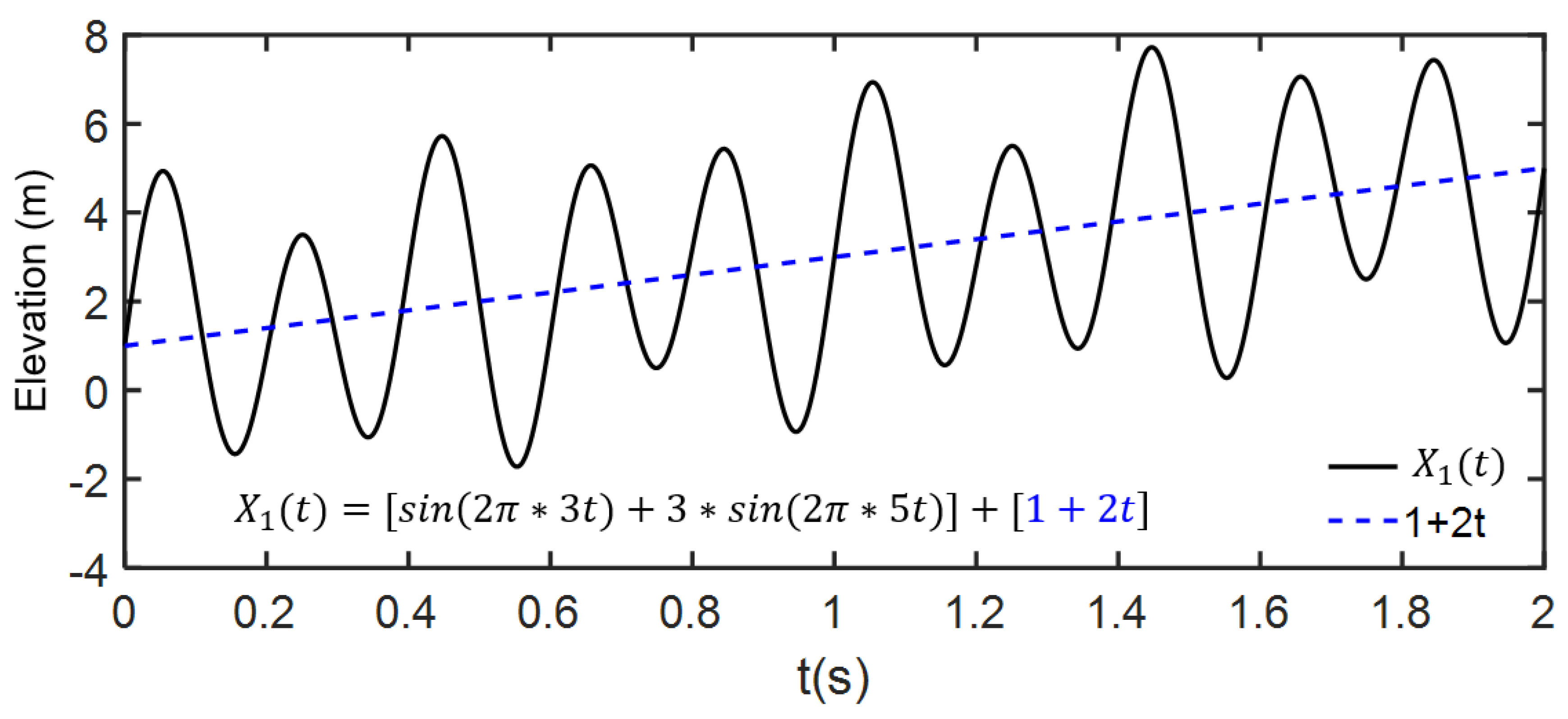
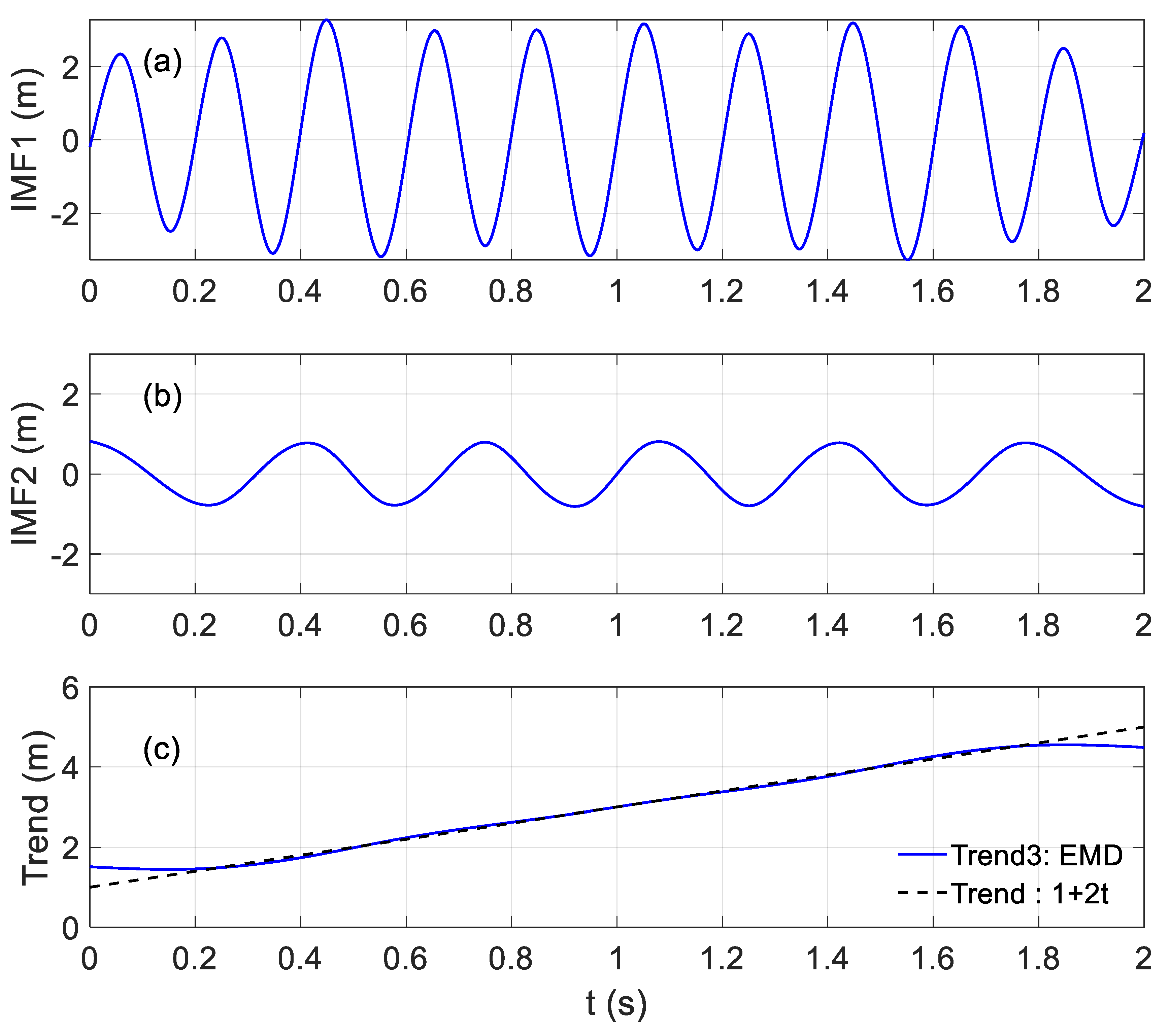
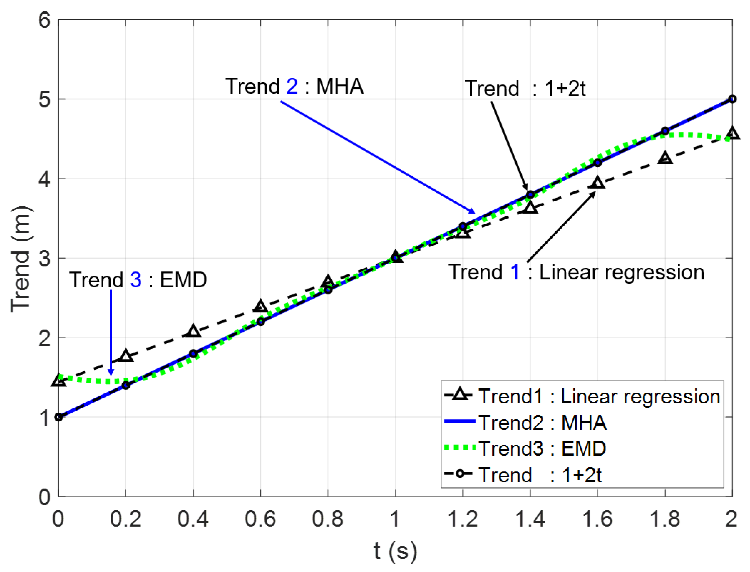
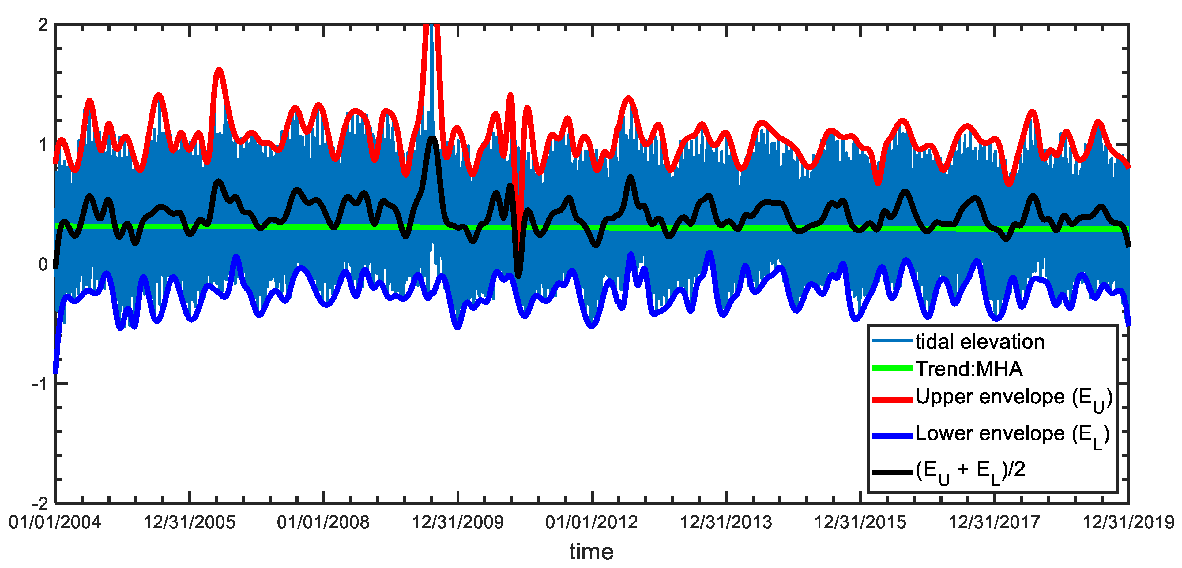
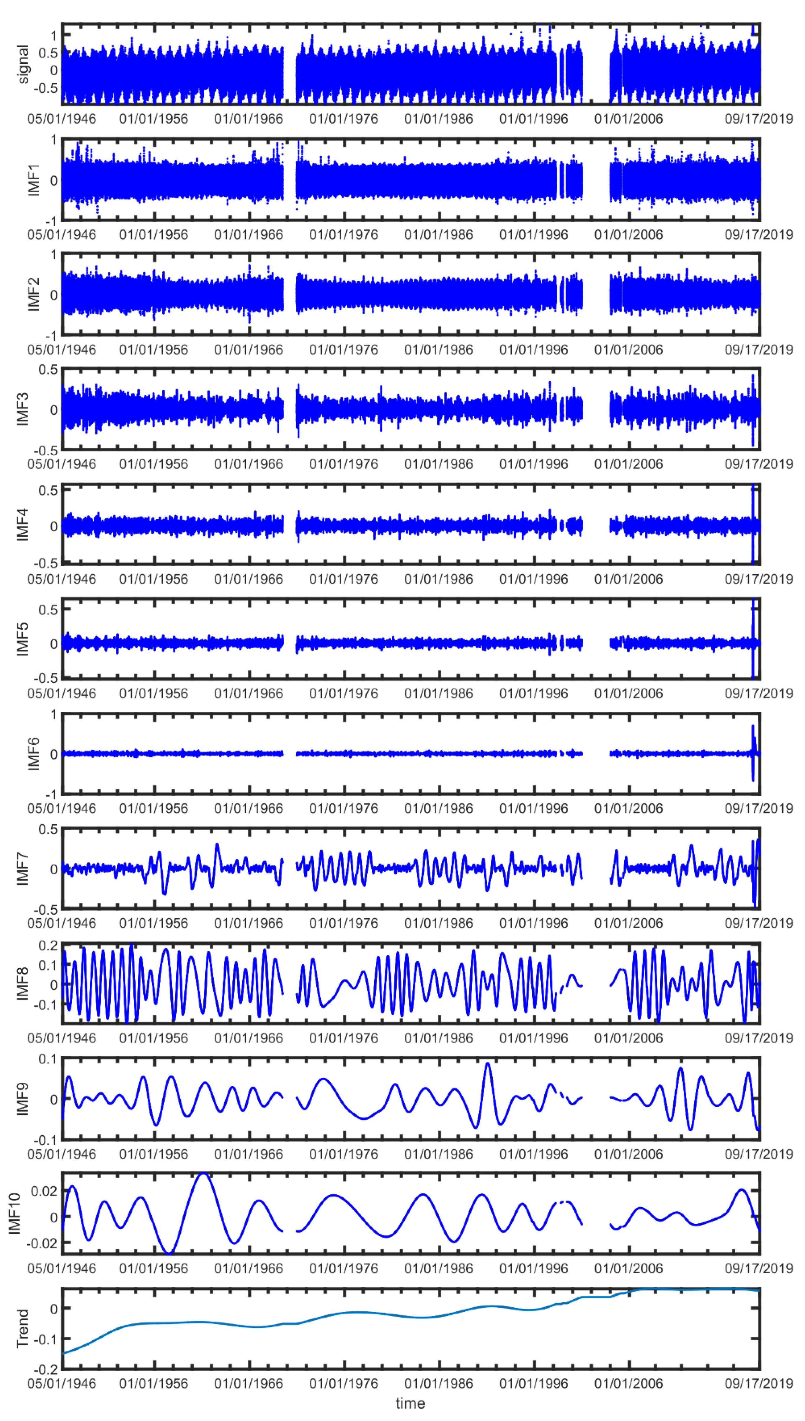
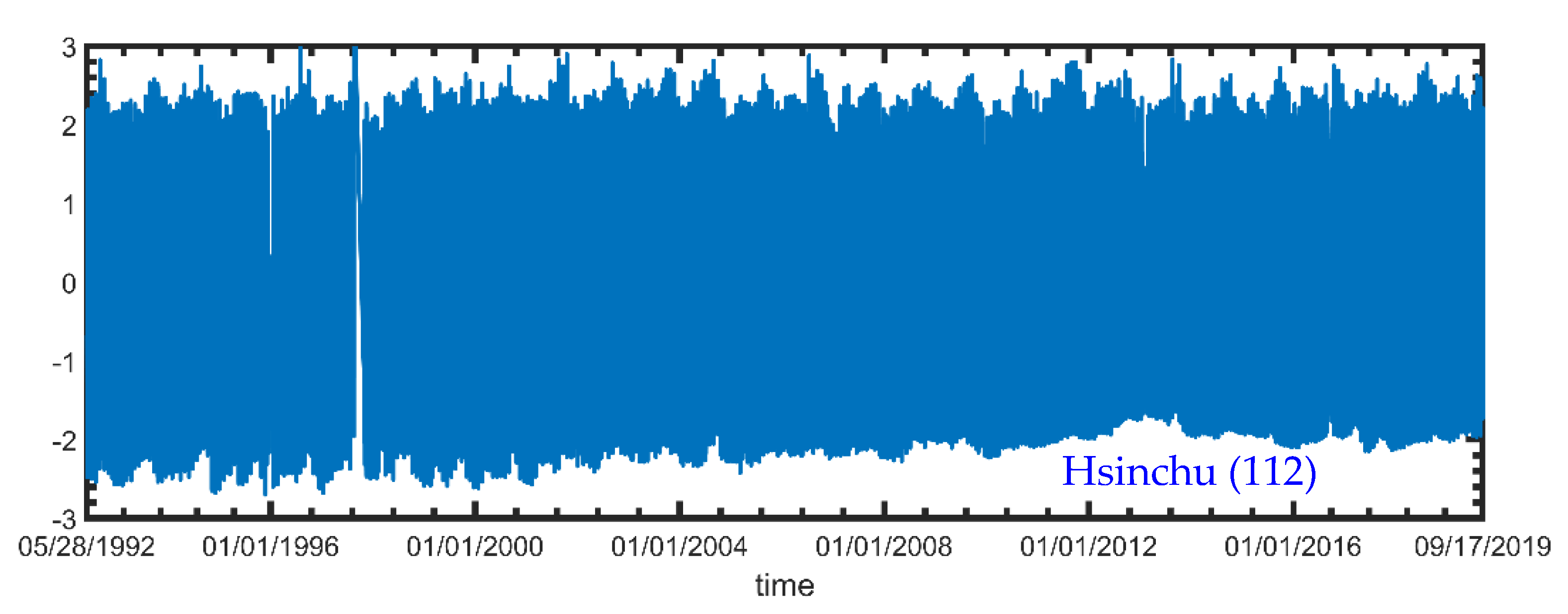
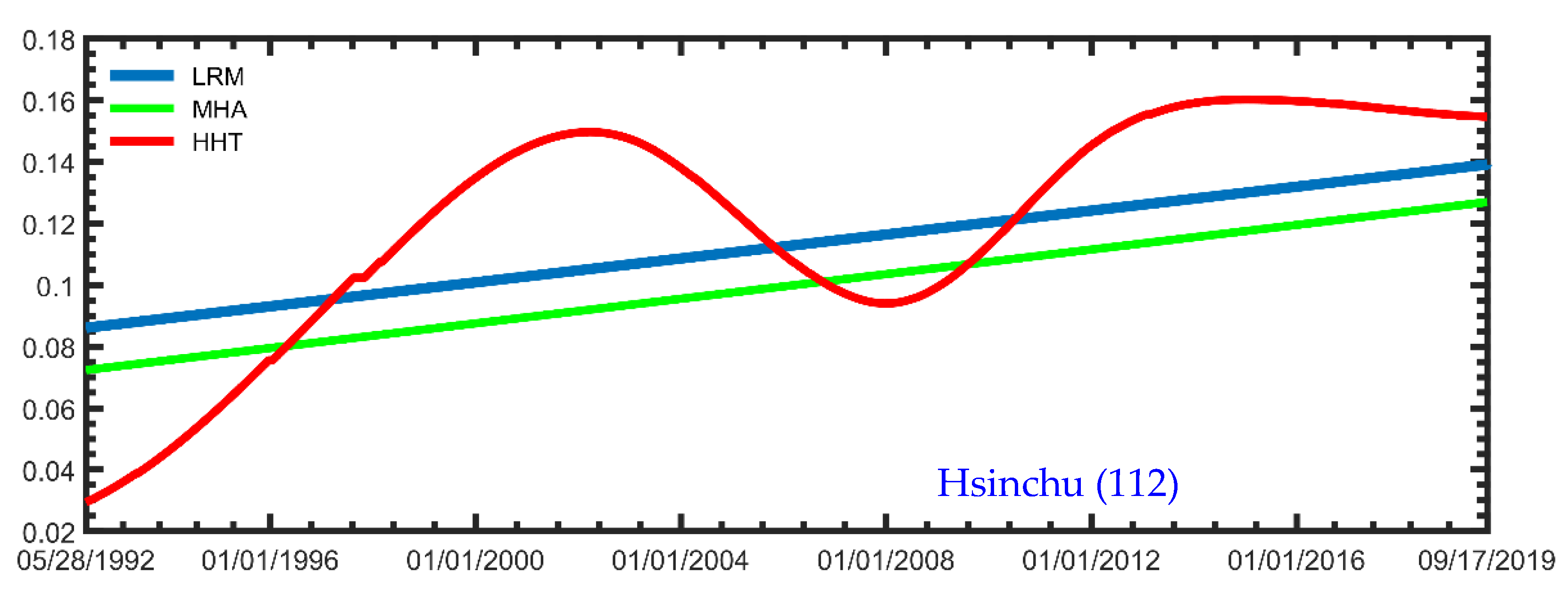
3.1. Examination of Temporal Function

In order to examine the advantages and disadvantages of these methods mentioned above, we construct a set of mixed-frequency signals. The temporal mixed-signal $X_1\left(t\right)$ is given by

$$X_1\left(t\right)=\left[{\alpha }_1\sin \left(2\pi \ast 3t\right)+{\alpha }_2\ast \sin \left(2\pi \ast 5t\right)\left]+\right[{\beta }_1+{\beta }_{2}t\right]$$

(3)

The coefficients${\alpha }_1=1$, ${\alpha }_2=3$, ${\beta }_0=1$, and ${\beta }_1=2$ are obtained by using LRM. Figure 1 shows the temporal variation of $X_1\left(t\right)$ (solid line) and the linear trend of $\left(1+2t\right)$ (dashed line). HHT is applied to find the envelope using the segmented endian-function-interpolation algorithm. The empirical-node-decomposition (EMD) algorithm is the core algorithm of HHT, and its primary purpose is to use the internal time scale of its change to analyze the energy directly. The process relies on the envelope-generation algorithm and the endpoint-spreading algorithm to find the envelope line using the segmented endian-function-interpolation algorithm. The EMD algorithm, based on the local characteristics of the data in the time domain, can decompose complex data into a limited and small number of intrinsic mode-function components. It is a data-driven self-adjusting time-frequency-analysis method that is also called sifting processing. As shown in Figure 2, a–c are IMF1, IMF2, and trend, respectively. Comparing the trend decomposed from EMD with the correct solution (1 + 2t), we found a significant gap at the boundary between the two ends.

Figure 3 shows the $X_1\left(t\right)$ signal using different analysis methods to calculate the trend-change graph. In Figure 3, Trend 1 shows the linear-regression straight line ${\widehat{y}}_i=a+b{t}_i,$ where a = 1.4362 and b = 1.5638, obtained by LRM. This method is used in the most traditional analysis of SLR. Trend 2 shows the linear-variation trend by LRM and MHA. Trend 3 presents the results of EMD. It is noted that the correct solution of the trend change in this example is 1 + 2t. Figure 3 shows that the result of Trend 1 is also following the trend (1 + 2t). Trend 3 is the analyzed result of the EMD method. In the EMD-screening process, the end swings of the upper- and lower-envelope curves would have excessive or very small amplitudes, resulting in end-effect problems. In this example, the most accurate trend is Trend 2, which divides the signal into period and trend signals and uses LRM to find the coefficient value. Figure 2 depicts two components of intrinsic mode functions (IMF1; IMF2) and the linear trend, respectively. Comparing the linear trend decomposed by making use of EMD, it is evident that ending swing occurs at two ends of the envelope. However, MHA is able to simulate $X_1\left(t\right)$ in a good agreement with the trend (1 + 2t).

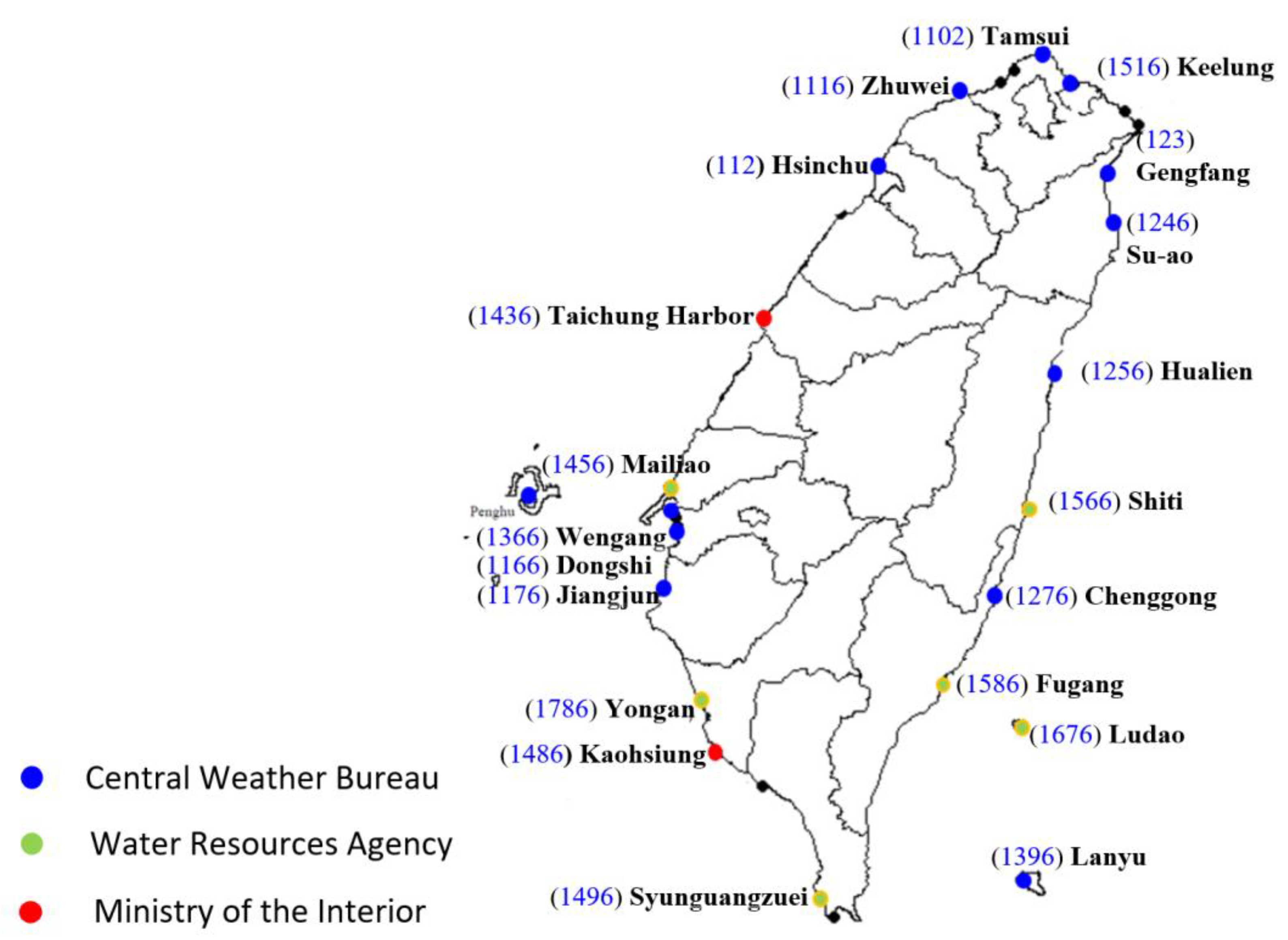
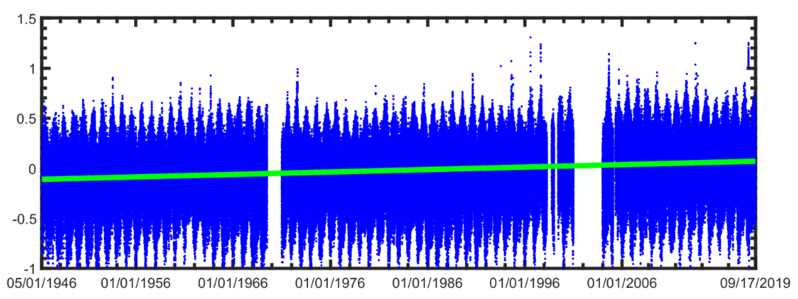
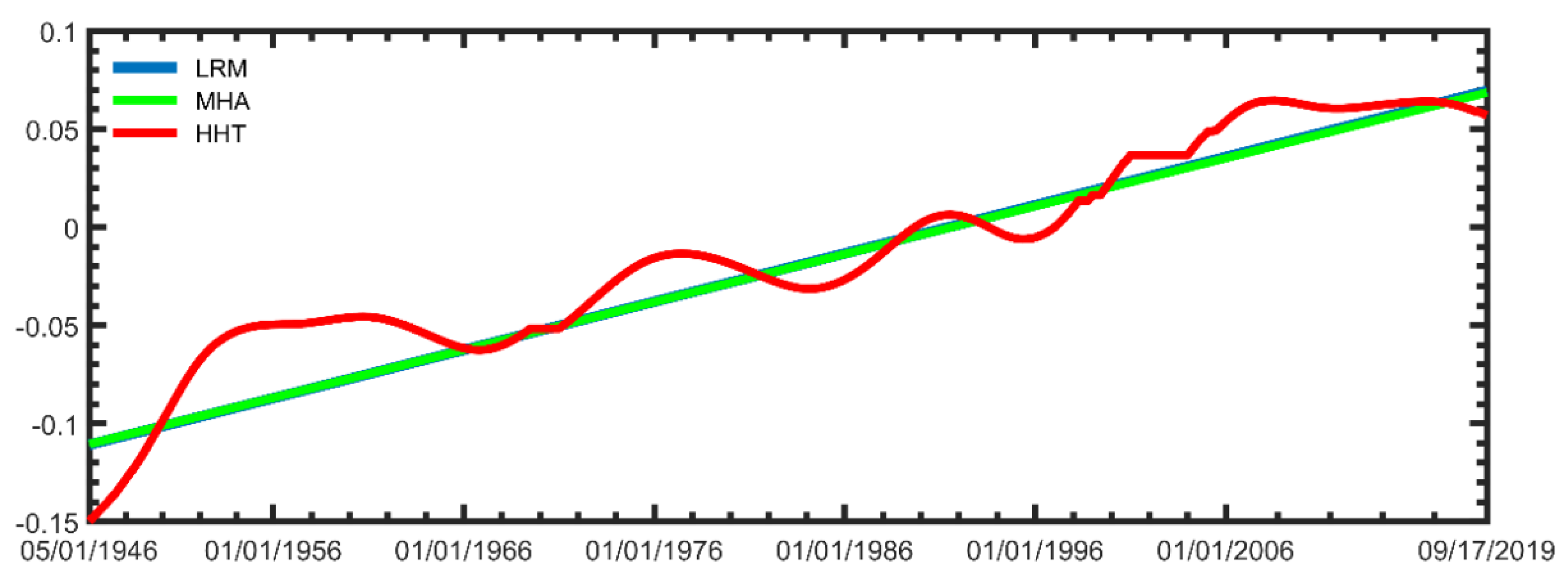
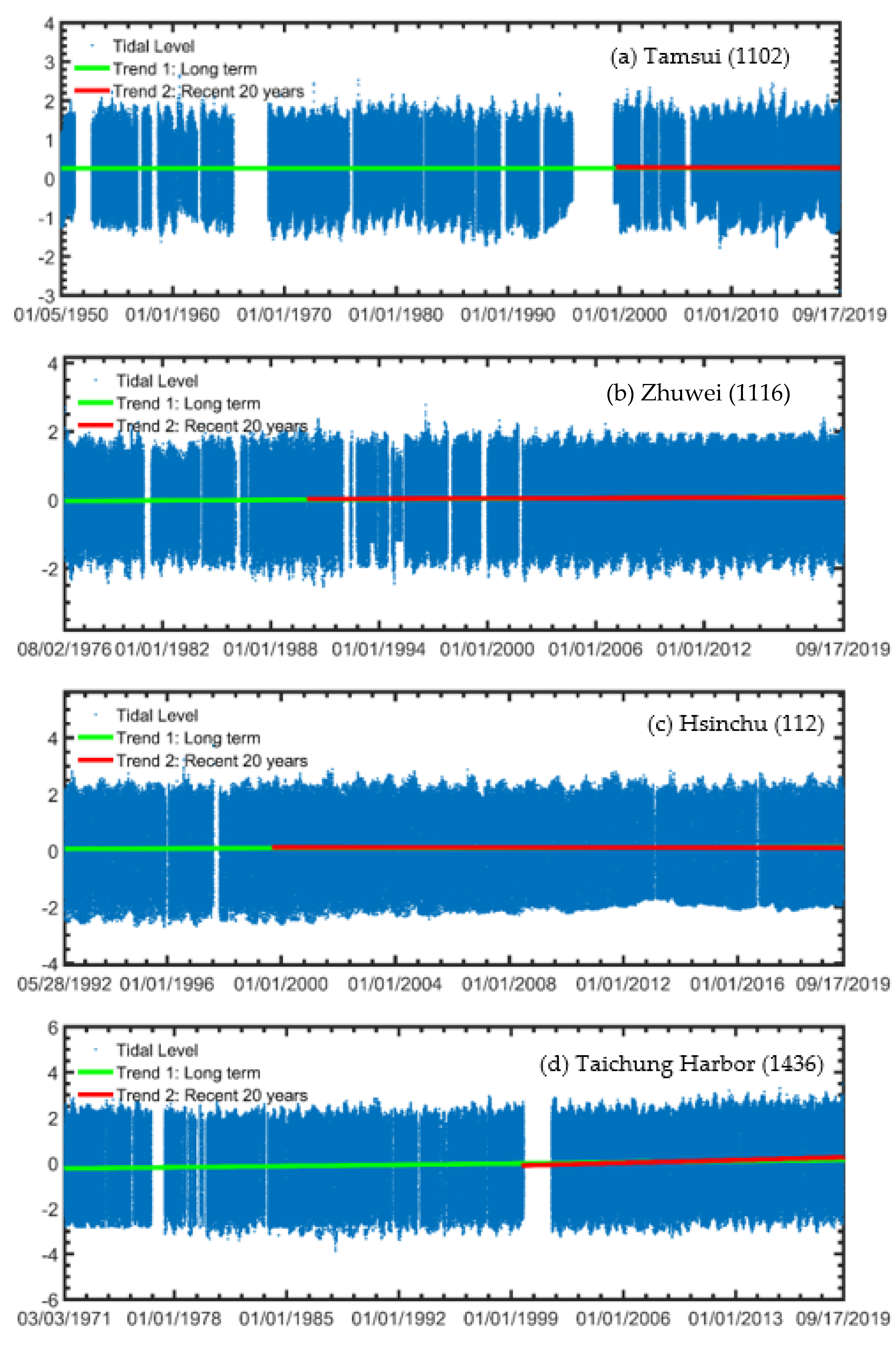
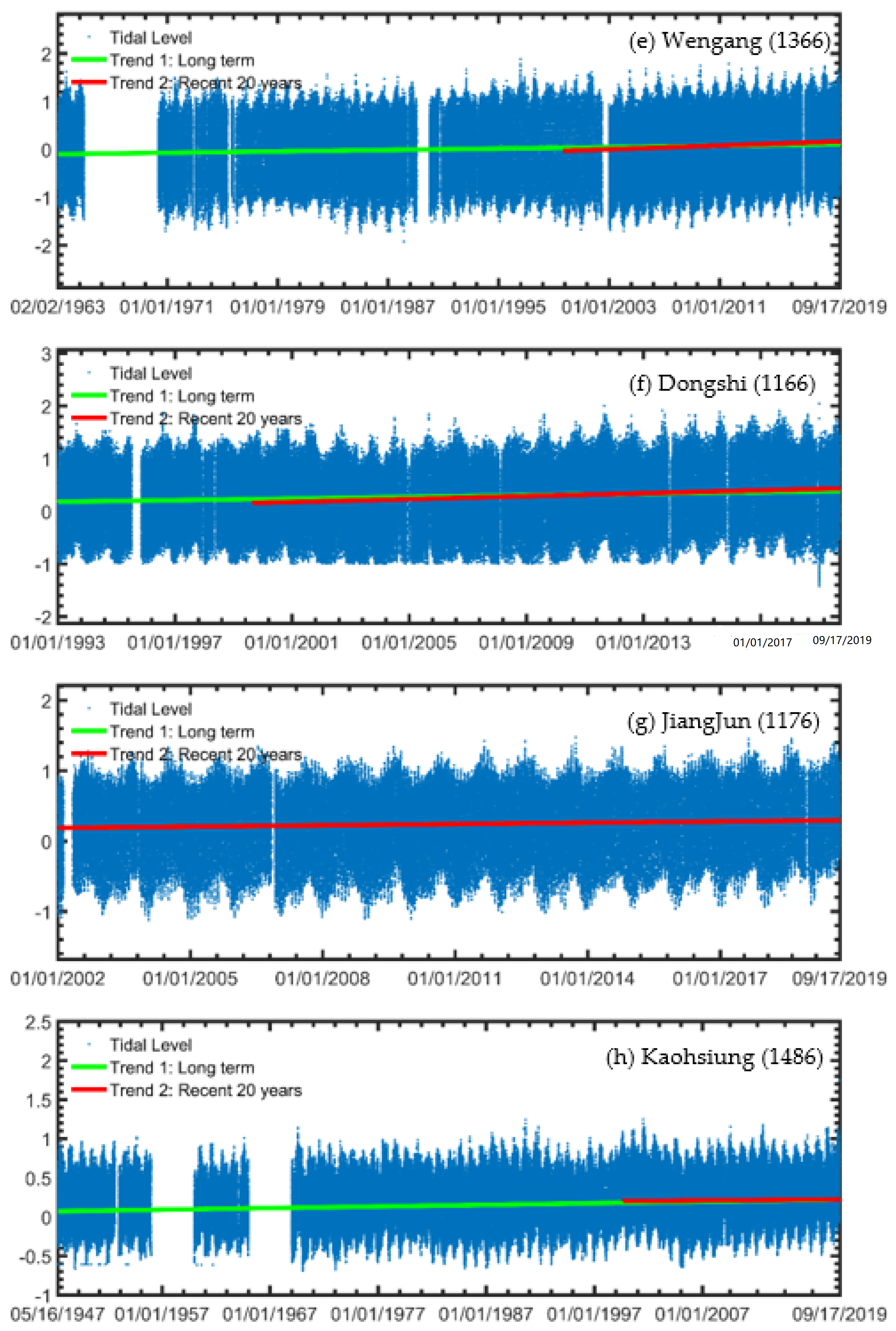
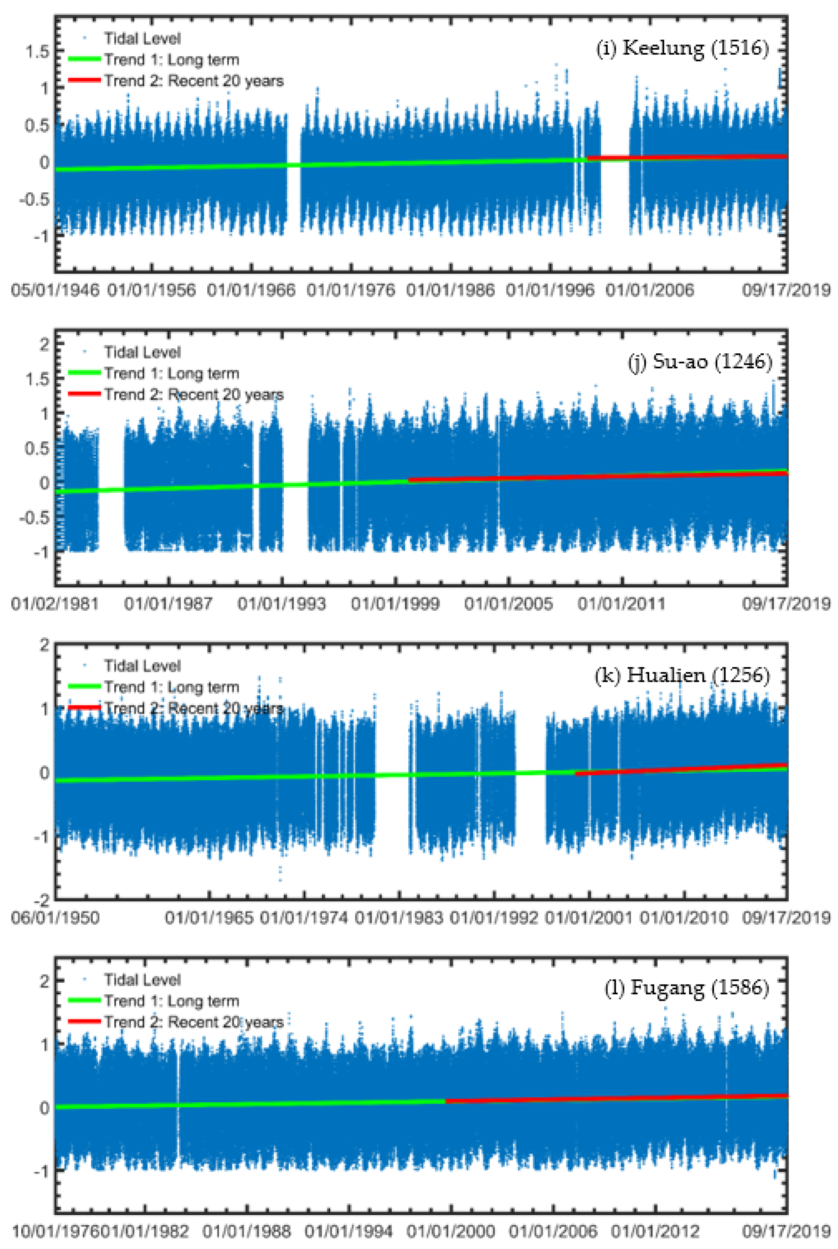
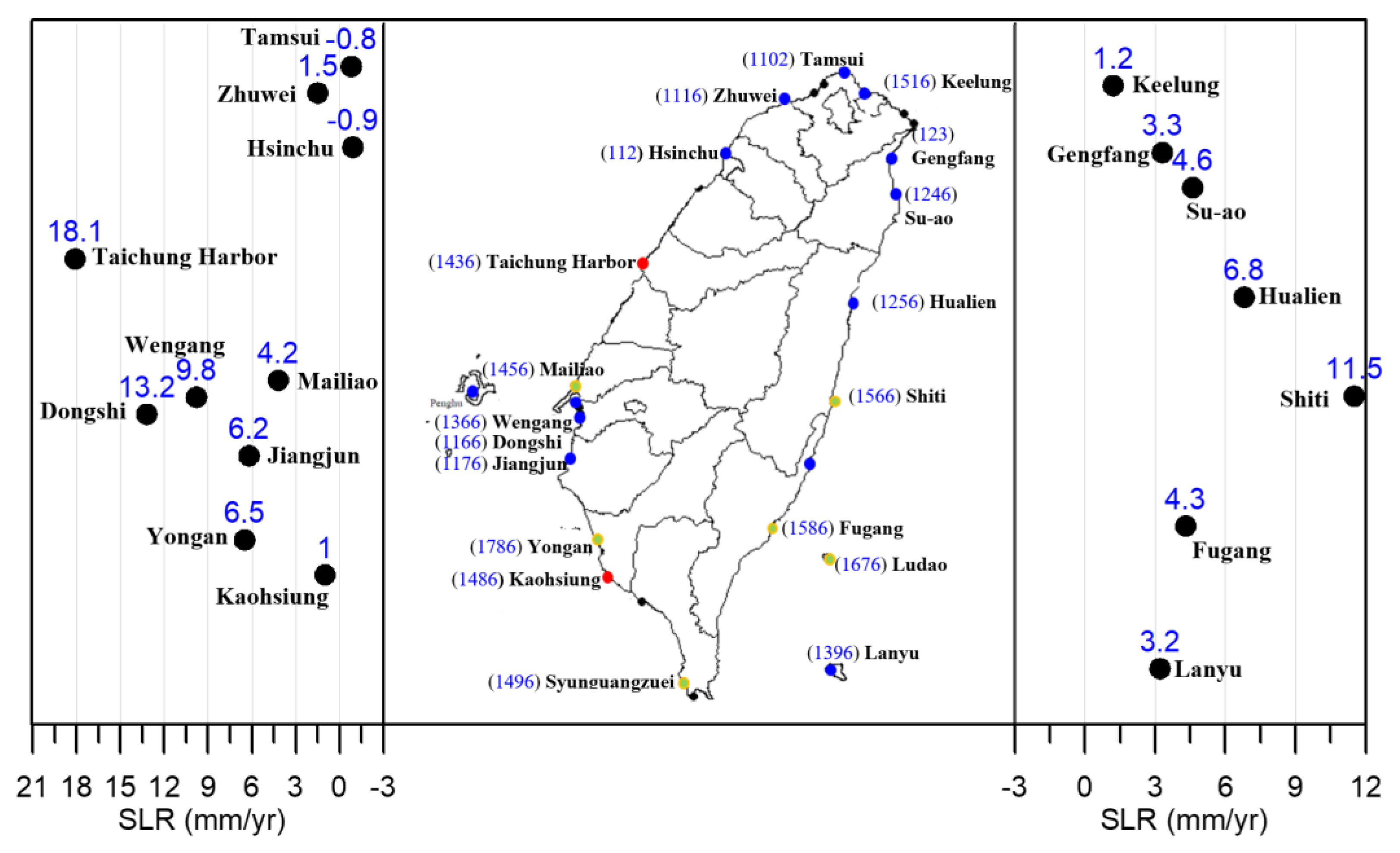
3.2. Tidal Data Analysis

A long-term measured database from the CWB, WRA (Water Resources Agency, New Taipei City, Taiwan), and Ministry of the Interior (MOI) is implemented to analyze the rising trend of SLR along the Taiwanese coast. The tidal stations located along the Taiwanese coast are shown in Figure 4. Note that the number in the parenthesis denotes the number of tidal stations. The number of the suffix, such as “6”, in the parenthesis represents the sonic-tidal-gauge stations while the others are pressure-gauge stations.

HHT combined with EMD is used to decompose a signal into a so-called intrinsic mode function (IMF), with a trend. The decomposition method can simply use the envelopes defined by the local maxima and minima separately. To explore the effect of the extreme tidal value on the envelope, we analyzed the tide level in Syunguangzuei, located in Pingtung County. Figure 5 presents the SLR increasing trend. It is evident that the envelope method can be easily influenced by extreme tidal levels.

Note that the end effect in the process of EMD is a significant swing. It appears at the endpoints of the signal, which ultimately affects the original significance of the decomposed signal. Serious problems of the spline fitting can occur near the ends, where the cubic spline fitting can have large swings. The end swings can eventually propagate inward and corrupt the whole data span, especially in the low-frequency components. An end effect occurs in HHT because the extreme value points need to be considered when using a cubic spline curve to calculate its envelope. In case of an endpoint without the extreme value point, it is abandoned and endpoints of the envelope and signals are different. According to the principle of EMD, several rounds of calculation of the envelope are needed to form the IMF components for each time. The error at the endpoints will gradually accumulate and eventually embody a significant deviation at the endpoints of IMF components. The end effect makes decomposition results lose practical significance to a certain extent.

This article analyzes the tidal-level records of various tidal stations. First, the data from the Keelung tidal station during the period from 1946 to 2019 was analyzed. Then, the data was decomposed into various intrinsic-mode functions (IMF) and trend signals by empirical-mode decomposition (EMD). The measured water level in Keelung from 1946 to 2019 is decomposed into 10 IMF and trend items, as shown in Figure 6, through EMD, and the tide data is decomposed into each time scale by EMD. This method expresses the original data as an intrinsic-mode-function (IMF) component, which has a clear physical meaning, a high degree of accuracy, and orthogonality and adaptability provide obvious local details with the time-frequency characteristics. The time scale of the tide signal is changed from high frequency to low frequency to analyze the local components. From each IMF, it is clear that the components of the tide are affected by astronomical tides. In terms of time scale, there is IMF 1 (12 h 25 min, semi-diurnal tides), IMF 2 (24 h 50 min, diurnal tides), and IMF 3 (30 days), which are affected by the moon’s gravity (time scales such as 15 days and 30 days). It is found from Figure 6 that the long-term sea-level fluctuation trend in the Keelung sea area is an upward trend.

Figure 6 is the Keelung tidal-trend-comparison graph with different trend analysis methods; Trend 1 uses linear-regression-line extrapolation to fit tide-level data; Trend 2 divides the tide-level data into periodic signals (60 harmonic components) and polynomials to fit the tide-level data; Trend 3 uses the EMD method in the HHT method to decompose each intrinsic-mode function (IMF) and trend. Figure 6 demonstrates the temporal variation of the water level at Keelung tidal station from 1946 to 2019. Figure 6 presents the analytical results for 10 IMFs and the increase in SLR by HHT. The swing from the first and ending points is significant. Figure 7 shows 60 harmonic components and the linear increasing trend of SLR. Figure 8 illustrates the variation of SLR by three different methods. In this figure, we find that the SLR rate is around 2.4 mm/yr.

Figure 9 shows the raw data observed at Hsinchu tidal station. From the envelope variation, it is clear to see that SLR increases significantly. Figure 10 displays the growing trend of SLR by different analysis methods. We also notice that LRM is limited to assess SLR as discussed by Huang et al. [19]. Likewise, HHT has the interest of conflicting for the ending swing. The previous method of assessing SLR was linear regression, such as Huang et al. [19]. However, linear regression and applying the least squares method cannot obtain the correct rising-sea-level trend. Furthermore, traditional harmonic-analysis methods cannot precisely analyze SLR.

The establishment and maintenance of tidal level observation are conducted by the Central Weather Bureau (CWB) of Taiwan. These data are available to public users for doing relative research on SLR. In this paper, the CWB database is used for the analysis and prediction of SLR. The present paper only focuses on the analysis and prediction of SLR on the basis of the long-term tidal database.

Table 1. Analysis of SLR rate at four different tidal stations.

Tidal Station	Time Period	Long-Term		Recent 20-Year
		SLR (mm/yr)	R2	SLR (mm/yr)	R2
Tamsui (1102)	1950/01/04~2019/09/17	0.1	0.91	−0.8	0.94
Zhuwei (1116)	1976/08/02~2019/09/17	2.7	0.97	1.5	0.98
Hsinchu (112)	1992/05/27~2019/09/17	2.0	0.98	−0.9	0.98
Taichung Harbor (1436)	1971/03/01~2019/09/17	7.8	0.94	18.1	0.99
Mailiao (1456)	2005/10/01~2019/09/17	X	X	4.2	0.99
Wengang (1366)	1963/02/02~2019/09/17	3.6	0.92	9.8	0.96
Dongshi (1166)	1993/01/01~2019/09/17	8.0	0.95	13.2	0.95
Jiangjun (1176)	2002/01/01~2019/09/17	6.2	0.95	6.2	0.95
Yongan (1786)	2004/01/01~2019/09/17	X	X	6.5	0.91
Kaohsiung (1486)	1947/05/16~2019/09/17	2.0	0.84	1.0	0.86
Keelung (1516)	1946/05/01~2019/09/17	2.4	0.87	1.2	0.91
Gengfan (123)	1976/05/01~2008/05/29	X	X	3.3	0.90
Su-ao (1246)	1981/01/01~2019/09/17	7.1	0.94	4.6	0.95
Hualien (1256)	1950/06/01~2019/09/17	2.6	0.91	6.8	0.94
Shiti (1566)	2004/01/01~2019/09/17	X	X	11.5	0.96
Fugang (1586)	1976/10/01~2019/09/17	3.8	0.91	4.3	0.94
Lanyu (1396)	1992/07/23~2019/09/17	3.5	0.92	3.2	0.94

Note: only when it has been more than 20 years can it be defined as long-term, e.g., X: it has been less than 20 years, so there is no calculation.

presents the long-term and recent 20-year variation of SLR by the MHA method. Note that the linear increase in SLR is in the range of −0.9 mm/yr and 18.1 mm/yr. We also notice that MHA has higher correlation coefficients, indicating that the method is applicable in the analysis and prediction of SLR. The establishment and maintenance of the tidal-level database are conducted by the Central Weather Bureau (CWB). These data are available to public users for research. In this paper, the CWB database is used for the analysis and prediction of SLR. The present paper only focuses on the analysis and prediction of SLR on the basis of the long-term tidal database.

We provide GPS data on the changes in the ground level of the observation points, based on the analyzed results by Ching et al. [20]. Subtraction of GPS readings from the readings of tidal stations is performed. Processing using various methods is conducted, and a comparison of the effect due to changes in the benchmark for some stations is discussed and presented in

Table 2. SLR rate corrected for vertical-surface change at tidal stations.

Tidal Station	Annual Ascent Rate in Past 20 Years (mm/yr)	Vertical-Change Rate of Surface GPS (mm/yr)	GPS-Measurement Time	SLR-Rise Rate for Sea-Level Correction of Vertical-Ground Change (mm/yr)
Keelung (1516)	1.2	−1.63 ± 0.09	2002/01–2012/12	−0.4
Jiangjun (1176)	6.2	−7.91 ± 0.05	2001/12–2012/09	−1.71
Kaohsiung (1486)	1.03	−0.91 ± 0.07	2004/01–2012/08	0.12
Syunguangzuei (1496)	5.0	−3.55 ± 0.12	2001/12–2012/09	1.45
Su-ao (1246)	4.6	−4.63 ± 0.12	2002/01–2012/08	−0.03
Hualien (1256)	6.83	−5.15 ± 0.13	2002/01–2012/12	1.73
Fugang (1586)	4.3	−3.89 ± 0.07	2003/12–2012/12	0.41

Note: GPS data is from Ching et al. [20].

. On the other hand, we analyze of the SLR rate at all 17 tidal stations, as shown in Table 1. Figure 11 demonstrates the SLR observations and the long- or short-term trend of SLR at different stations. The blue dot denotes the observed tide-level data, the green line represents the long-term change trend of SLR, and the red line is the sea-level-change trend from 1999 to 2019. According to the observed database from all tidal stations in Taiwan, it is reasonable to define the 20-year database as the long-term SLR rate, in the present paper. The results at all tidal stations using modified-harmonic analysis (MHA) are demonstrated in Figure 11. It is evident that the analyzed results of periodic components and the linear-growing trend of SLR are meaningful. From these figures, we conclude that MHA has the advantage of analyzing the SLR rate, consistent with realistic characteristic tidal variations.

The results from Table 1 show that (1) Taiwan’s SLR rate as a “long-term-rise rate” is more than two times faster than the global average for these tidal stations: Taichung Harbor, Dongshi, Jiangjun, Su-ao, etc.; (2) Taiwan’s SLR rate is more than two times faster than the global average for the past 20 years, around tidal stations such as Taichung Port, Wengang, Dongshi, Jiangjun, Yongan, Hualien Port, and Shiti.

Kuo et al. [34] studied the increase in SLR around the Taiwanese coast from 2002–2011 using both SA data and tide-gauge data. The report pointed out that the absolute SLR change rate is −1~2 mm/yr and 4~8 mm/yr in northern and southern Taiwan, respectively. The results from Table 1, Figure 11, and Figure 12 also show that SLR is about −1~2 mm/yr and 1~6.5 mm/yr in northern and southern Taiwan, respectively.

In this paper, the SLR rates of all tide-level stations are combined into (Figure 12) the trend chart of sea-level changes at tide-level stations around Taiwan in the past 20 years. The fastest rate of SLR on the west coast is Taichung Port at 18.1 mm/yr, followed by Dongshi tidal station at 13.2 mm/yr. The SLR rate on the east coast is the fastest at Shiti at 11.5 mm/yr, followed by Hualien tidal station at 6.8 mm/yr. The distribution of SLR rates on the east and west coasts is very similar to the distribution of the tidal range in Taiwan. The rapid rise of the benchmark at the tidal stations of Wengang and Dongshi is because the area is affected by stratum subsidence, and the annual surface subsidence of Wengang tidal station is about 14 mm (Ching et al. [20]). The tidal stations in Wengang and Dongshi cause SLR to decline, based on the amount of liquid water on land, due to groundwater over pumping.

The analysis of the case in this article has not corrected for the crustal changes or stratum-subsidence factors, so it is higher than the global rate of rise. Ching et al. [20] used the Global Positioning System (GPS), continuous observation stations, and precise leveling data to estimate the vertical-change rate of the surface of Taiwan’s main island, and they proposed that the amount of vertical change in the surface of Taiwan’s southeastern and southwestern regions is higher than the sea-level fluctuation around Taiwan. This is because the vertical-fluctuation signal of the surface included in the tidal station will significantly affect the sea-surface-rise rate estimated by the tidal-station data.

This article analyzes the tide level without considering the influence of the abrupt change of the surface of the tide station. This article refers to the global satellite-positioning-system (GPS) observation-station data of Ching et al. [20]. The system (GPS) observation station is compared with the benchmarking points, and the SLR rate after the vertical-change rate of the surface is considered. The results are shown in Table 2. The SLR rate of the tide station is corrected by considering the vertical-change rate of the surface, and the SLR rate of the tide station around the island of Taiwan, after the correction, tends to be the same. Based on the literature, as mentioned earlier, by directly using the data from the tidal stations around Taiwan that have not corrected for the vertical-surface fluctuations and the estimated absolute sea-surface-rise rate, the signal of the vertical-surface fluctuation will significantly affect the estimation results of the sea-surface-rise rate.

The analysis results of this article are different from those of past scholars, mainly because past scholars used linear regression to analyze the rate of SLR, and the analysis of this article uses an improved harmonic-analysis method, so there will be differences. In addition, this method is based on the LRM, so the analysis results will vary with the length of time that the data is selected for.

Table 1 and Figure 11 show the SLR trend of the records of the tidal stations around Taiwan coast. Analyzing the rate of SLR over the past 20 years shows that SLR continues to grow at stations such as Taichung Harbor, Wengang, Dongshi, Hualien, and Fugang. On the contrary, SLR is decelerating for these tidal stations: Keelung, Tamsui, Zhuwei, Hsinchu, Kaohsiung, Suao, and Lanyu.

Table 3. SLR rate using different databases and scenarios.

Databases and Scenarios	Increase in SLR from Min. to Max.
Tide gauge [8,22,23,31,32]	3.0 ± 0.7 mm/yr~3.1 ± 1.4 mm/yr
Satellite altimetry [6,11,13,14,15,22,24,33]	0.3 mm/yr~1.2 mm/yr
Ice melting [25,27,28,29]	0.21 mm/yr~0.74 mm/yr
Greenhouse effect and higher CO2-emissions scenarios [9,10,12,21,23,26]	0.11 mm/yr~8.9 mm/yr

presents a comparison of changes of SLR by using different databases and scenarios. It is interesting to note that the increase in SLR varies in the range of 0.11 mm/yr to 4.5 mm/yr. The present result is located within the interval of 1.03 mm/yr and 6.8 mm/yr. We, thus, conclude that different databases, scenarios, data lengths, analyzed methods, and locations will result in different results for an estimate of SLR. Further investigations are needed to keep the analysis and prediction of SLR ongoing, in the near future.

4. Conclusions

In this paper, we estimate the growing trend of SLR from the tidal-gauge measurements located in different sites of Taiwan. Different methods of analysis, such as the linear-regression method (LRM), Hilbert–Huang transform (HHT), and modified harmonic analysis (MHA) are used to estimate SLR and their applicability is discussed. Limitations of these methods are also compared and discussed via the analyzed results. MHA is the focus of the present paper. It has the advantage of precisely representing the tidal-harmonic motion as well as the long-term growing trend of SLR, even in the condition of data loss caused by mechanical failures or an anomaly. The analyzing results reveal that MHA is more applicable for estimating SLR than the commonly used methods.

We analyze the long-term growing trend of SLR from the measured tidal data provided by the meteorological bureau at different locations around the Taiwanese coast. Different methods are utilized to calculate SLR. Comparison of the analytical results shows that MHA is more reasonable to decompose the tide-level data into periodic signals (astronomical tides) and non-periodic (monotonic) trends.

Tidal data observed at different locations around the Taiwanese coast are used to evaluate the long-term and recent 20-year variation of SLR by the MHA method. It is found that the linear increase in SLR is within the range of −0.9 mm/yr and 18.1 mm/yr. The higher correlation coefficients indicate that MHA is applicable in the analysis and prediction of SLR. We, thus, conclude that MHA has the advantage of analyzing the SLR rate, consistent with realistic characteristic tidal variations. The most important analyzed results indicate that the recent 20-year SLR rate is within the range of −0.9 mm/yr and 18.1 mm/yr, using the tidal database observed at 17 stations along the Taiwanese coast. SLR is modified by adding the vertical-change rate of the benchmark. It is interesting to note that correction tends to reduce the bias of the variation trend of SLR.

References

1. Feenstra, J.F.; Burton, I.; Smtih, J.B.; Tol, R.S.J. Handbook on Methods for Climate Change Impact Assessment and Adaptation Strategies; United Nations Environment Program (UNEP): Nairobi, Kenya; University of Amsterdam: Amsterdam, The Netherland, 1998. [Google Scholar]
2. Maaskant, B.; Jonkman, S.N.; Bouwer, L.M. Future risk of flooding: An analysis of changes in potential loss of life in South Holland (The Netherlands). Environ. Sci. Policy 2009, 12, 157–169. [Google Scholar] [CrossRef]
3. Douglas, B.C. Chapter 3 Sea level change in the era of the recording tide gauge. Int. Geophys. 2001, 75, 37–64. [Google Scholar]
4. Mitrovica, J.X.; Tsimplis, M.E.; Davis, J.L.; Milne, G.A. Recent mass balance of polar ice sheets inferred from patterns of global sea level change. Nature 2001, 409, 1026–1029. [Google Scholar] [CrossRef] [PubMed]
5. Church, J.A.; White, N.J.; Coleman, R.; Lambeck, K.; Mitrovica, J.X. Estimates of regional distribution of SLR over the 1950–2000 period. J. Clim. 2004, 17, 2609–2625. [Google Scholar] [CrossRef]
6. Church, J.; White, N.J. SLR from the late 19th to the Early 21st Century. Surv. Geophys. 2011, 32, 585–602. [Google Scholar] [CrossRef] [Green Version]
7. Shum, C.K.; Kuo, C.Y. Observation and geophysical causes of present-day SLR. In Climate Change and Food Security in South Asia; Springer: Dordrecht, The Netherland, 2011; pp. 85–104. [Google Scholar]
8. Merrifield, M.A.; Merrifield, S.T.; Mitchum, G.T. An Anomalous Recent Acceleration of Global SLR. J. Clim. 2009, 22, 5772–5781. [Google Scholar] [CrossRef] [Green Version]
9. Intergovernmental Panel on Climate Change (IPCC). Climate Change 2013: The Physical Science Basis. Contribution of Working Group I to the Fifth Assessment Report of the Summary for Policymakers; Stocker, T.F., Qin, D., Plattner, G.-K., Tignor, M., Allen, S.K., Boschung, J., Nauels, A., Xia, Y., Bex, V., Midgley, P.M., Eds.; Cambridge University Press: Cambridge, UK; New York, NY, USA, 2013; Available online: https://www.ipcc.ch/report/ar5/wg1/ (accessed on 14 April 2022).
10. Intergovernmental Panel on Climate Change (IPCC). Climate Change 2021: The Physical Science Basis. Contribution of Working Group I to the Fifth Assessment Report of the Summary for Policymakers; Masson-Delmotte, V., Zhai, P., Pirani, A., Connors, S.L., Péan, C., Berger, S., Caud, N., Chen, Y., Goldfarb, L., Gomis, M.I., et al., Eds.; Cambridge University Press: Cambridge, UK; New York, NY, USA, 2021; Available online: https://www.ipcc.ch/report/ar6/wg1/ (accessed on 14 April 2022).
11. Nerem, R.S.; Beckley, B.D.; Fasullo, J.T.; Hamlington, B.D.; Masters, D.; Mitchum, G.T. Climate-change–driven accelerated sea-level rise detected in the altimeter era. Proc. Natl. Acad. Sci. USA 2018, 115, 2022–2025. [Google Scholar] [CrossRef] [Green Version]
12. Manabe, S.; Stouffer, R.J. Century-scale effects of increased atmospheric CO2 on the ocean–atmosphere system. Nature 1993, 364, 215–218. [Google Scholar] [CrossRef]
13. Nicholls, R.J.; Cazenave, A. Sea-level rise and its impact on coastal zones. Science 2010, 328, 1517–1520. [Google Scholar] [CrossRef]
14. Xu, S.S.; Zou, J.C.; Chen, M.X. North Pacific Sea level change and its impact factors during 1993–2006. Period. Ocean Univ. China 2010, 40, 24–32. (In Chinese) [Google Scholar]
15. Ablain, M.; Cazenave, A.; Valladeau, G.; Guinehut, S. A new assessment of the error budget of global mean sea level rate estimated by satellite altimetry over 1993–2009. Ocean Sci. 2009, 5, 193–201. [Google Scholar] [CrossRef] [Green Version]
16. Huang, N.E.; Shen, Z.; Long, S.R.; Wu, M.C.; Shih, H.H.; Zheng, Q.; Yen, N.C.; Tung, C.C.; Liu, H.H. The empirical mode decomposition and the Hilbert spectrum for nonlinear and non-stationary time series analysis. Proc. R. Soc. Lond. Ser. A 1998, 454, 903–995. [Google Scholar] [CrossRef]
17. Huang, N.E.; Shen, Z.; Long, S.R. A new view of nonlinear water waves: The Hilbert spectrum. Annu. Rev. Fluid Mech. 1999, 31, 417–457. [Google Scholar] [CrossRef] [Green Version]
18. Wu, Z.; Huang, N.E. Ensemble Empirical Mode Decomposition: A Noise-Assisted Data Analysis Method; Technol Report No. 193; Center for Ocean-Land-Atmosphere Studies: Fairfax, VA, USA, 2005. [Google Scholar]
19. Huang, Z.; Zong, Y.; Zhang, W. Coastal Inundation due to sea level rise in the Pearl River delta, China. Nat. Hazards 2004, 33, 247–264. [Google Scholar] [CrossRef] [Green Version]
20. Ching, K.E.; Hsieh, M.L.; Johnson, K.M.; Chen, K.H.; Rau, R.J.; Ying, M. Modern vertical deformation rates and mountain building in Taiwan from precise leveling and continuous GPS observations, 2000–2008. J. Geophys. Res. 2011, 116, B08406. [Google Scholar] [CrossRef]
21. Kulp, S.A.; Strauss, B.H. New elevation data triple estimates of global vulnerability to sea-level rise and coastal flooding. Nat. Commun. 2019, 10, 4844. [Google Scholar] [CrossRef] [Green Version]
22. Hay, C.C.; Morrow, E.; Kopp, R.E.; Mitrovica, J.X. Probabilistic reanalysis of twentieth-century sea-level rise. Nature 2015, 517, 481–484. [Google Scholar] [CrossRef]
23. Dangendorf, S.; Marcos, M.; Wöppelmann, G.; Conrad, C.P.; Frederikse, T.; Riva, R. Reassessment of 20th century global mean sea level rise. Proc. Natl. Acad. Sci. USA 2017, 114, 5946–5951. [Google Scholar] [CrossRef] [Green Version]
24. Kopp, R.E.; Horton, R.M.; Little, C.M.; Mitrovica, J.X.; Oppenheimer, M.; Rasmussen, D.J.; Strauss, B.H.; Tebaldi, C. Probabilistic 21st and 22nd century sea-level projections at a global network of tide-gauge sites. Earth’s Future 2014, 2, 383–406. [Google Scholar] [CrossRef]
25. Kopp, R.E.; DeConto, R.M.; Bader, D.A.; Hay, C.C.; Horton, R.M.; Kulp, S.; Oppenheimer, M.; Pollard, D.; Strauss, B.H. Evolving Understanding of Antarctic Ice-Sheet Physics and Ambiguity in Probabilistic Sea-Level Projections. Earth’s Future 2017, 5, 1217–1233. [Google Scholar] [CrossRef] [Green Version]
26. Nauels, A.; Rogelj, J.; Schleussner, C.F.; Meinshausen, M.; Mengel, M. Linking sea level rise and socioeconomic indicators under the Shared Socioeconomic Pathways. Environ. Res. Lett. 2017, 12, 114002. [Google Scholar] [CrossRef] [Green Version]
27. Wong, T.E.; Bakker, A.M.; Keller, K. Impacts of Antarctic fast dynamics on sea-level projections and coastal flood defense. Clim. Chang. 2017, 144, 347–364. [Google Scholar] [CrossRef]
28. Le Bars, D.; Drijfhout, S.; de Vries, H. A high-end sea level rise probabilistic projection including rapid Antarctic ice sheet mass loss. Environ. Res. Lett. 2017, 12, 044013. [Google Scholar] [CrossRef]
29. Bamber, J.L.; Oppenheimer, M.; Kopp, R.E.; Aspinall, W.P.; Cooke, R.M. Ice sheet contributions to future sea-level rise from structured expert judgment. Proc. Natl. Acad. Sci. USA 2019, 116, 11195–11200. [Google Scholar] [CrossRef] [PubMed] [Green Version]
30. Visser, H.; Dangendorf, S.; Petersen, A.C. A review of trend models applied to sea level data with reference to the “acceleration-deceleration debate”. J. Geophys. Res. Ocean. 2015, 120, 3873–3895. [Google Scholar] [CrossRef]
31. Becker, M.; Karpytchev, M.; Lennartz-Sassinek, S. Long-term sea level trends: Natural or anthropogenic? Geophys. Res. Lett. 2014, 41, 5571–5580. [Google Scholar] [CrossRef] [Green Version]
32. Dangendorf, S.; Rybski, D.; Mudersbach, C.; Müller, A.; Kaufmann, E.; Zorita, E.; Jensen, J. Evidence for long-term memory in sea level. Geophys. Res. Lett. 2014, 41, 5564–5571. [Google Scholar] [CrossRef] [Green Version]
33. Llovel, W.; Guinehut, S.; Cazenave, A. Regional and interannual variability in sea level over 2002-2009 based on satellite altimetry, Argo float data and GRACE ocean mass. Ocean Dyn. 2010, 60, 1193–1204. [Google Scholar] [CrossRef]
34. Kuo, C.Y.; Lin, L.C.; Lan, W.H.; Juang, W.J.; Lee, C.Y. Projection of Future Sea Level Changes around Taiwan; MOTC Technol Report No. 105-023-7863; Institute of Transportation: Taipei, Taiwan, 2016. (In Chinese)
Figure 1. Time series graph of X 1 t is given by Equation (3).
Sustainability 14 07291 g001
Figure 2. X 1 t signal trend applying EMD method.
Sustainability 14 07291 g002
Figure 3. The trend change of different analysis methods on X 1 t signal.
Sustainability 14 07291 g003
Figure 4. Locations of tidal stations around Taiwan.
Sustainability 14 07291 g004
Figure 5. Sea level trend of Syunguangzuei obtained by the envelope method (unit: m).
Sustainability 14 07291 g005
Figure 6. IMF and trend chart of Keelung tide-level obtained using EMD (unit: m).
Sustainability 14 07291 g006
Figure 7. Harmonic components and increasing trend of tidal motion at Keelung station (unit: m).
Sustainability 14 07291 g007
Figure 8. Long-term growing SLR at Keelung station (unit: m).
Sustainability 14 07291 g008
Figure 9. Row of tidal-elevation data observed at Hsinchu station (unit: m).
Sustainability 14 07291 g009
Figure 10. Increasing trend of SLR by different methods of LRM, MHA, and HHT.
Sustainability 14 07291 g010
Figure 11. Long-terme tidal variation of harmonic components and linear increase in SLR by the MHA method.
Sustainability 14 07291 g011aSustainability 14 07291 g011bSustainability 14 07291 g011c
Figure 12. The trend chart of sea-level change around the tidal stations of Taiwan in the past 20 years.
Sustainability 14 07291 g012