Research and Analysis on the Influencing Factors of China’s Carbon Emissions Based on a Panel Quantile Model

Abstract

Since the beginning of the new century, China’s carbon emissions have increased significantly, and the country has become the world’s largest carbon emitter. Therefore, determining the influencing factors of carbon emissions is an important issue for policymakers. Based on the panel data of 30 provinces and cities across the country from 2000 to 2018, this study empirically tested how per capita disposable income, industrial structure, urbanization level, average family size, and technological innovation level impacts carbon emissions at different quantile levels by using the panel quantile STIRPAT model. The results showed that per capita disposable income and industrial structure had significant promoting effects on carbon emissions, while urbanization level, average family size, and technological innovation level had significant inhibitory effects on carbon emissions. The main thing is that the emission distributions of the 10th and 90th quantiles of the independent variables were quite different, which shows that the influence of each factor on carbon emissions has obvious heterogeneity at different levels. Specifically, the impact of per capita disposable income and technological innovation level on carbon emissions in low carbon emission areas were higher than that in high carbon emission areas, and the impact of industrial structure, urbanization level, and average household size on carbon emissions in high carbon emission areas was higher. Finally, specific policy implications are provided based on these results.

1. Introduction

With the rapid development of the world economy, the environmental problems caused by the excessive consumption of resources and the unsustainable development model are becoming more and more prominent. Especially since the beginning of the twenty-first century, environmental issues have become a major concern for all economies. Greenhouse gases, especially carbon emissions associated with human activities, are considered to be the main cause of this problem. Controlling carbon emissions and developing a low-carbon economy have become the focus of global attention. Based on current policy trends, global energy-related carbon dioxide (CO₂) emissions will now increase over the next 30 years. Between 2020 and 2050, the total energy-related CO₂ emissions are projected to increase by 5% in OECD countries and 35% in non-OECD countries (International Energy Outlook 2021), so the international community is facing a very significant challenge, especially when emissions cross geographic boundaries. In particular, some developing countries such as China are facing enormous pressure from the international community. Data show that in 2007, China’s carbon emissions surpassed that of the United States and that China became the world’s largest carbon emitter. China has made great efforts to reduce carbon emissions and has pledged to reach the carbon peak by 2030 and achieve carbon neutrality by 2060, demonstrating China’s determination to reduce carbon emissions.

Since the reform and opening up, China’s economy has been growing at an annual rate of nearly 10%, and in 2010 it surpassed Japan to become the world’s second largest economy. With the rapid development of China’s economy, the level of the material wealth of residents has also been improved. The national per capita disposable income was 171 yuan in 1978, which is equivalent to 5301 yuan in 2019 considering inflation, and the national per capita disposable income in 2019 was 30,733 yuan, which has increased significantly in the past few decades. According to the environmental curve theory, before reaching the inflection point, when the per capita income increases, the environmental pollution will gradually increase. With the increase in income level, people began to expend more, and more and more people began to live in cities. According to the central place theory put forward by the German urban geographer W. Christaller, he believes that economic activities are the main factors for the formation and development of cities. At present, the economic exchanges between regions in China are becoming more and more frequent, so the level of urbanization continues to expand. Especially in recent years, the continuous relaxation of urban settlement policies and the gradual improvement of the housing market system and security system have created conditions for residents to live in cities. The increasingly widespread migration has dispersed family members who used to live in one household, which has led to a gradual reduction in the average family size in our country. At the same time, China’s industrial structure has been continuously adjusted since the reform and opening up. Industrial structure refers to the industrial composition of a country or region, that is, the state of resource allocation among industries, the level of industrial development, that is, the proportion of each industry, and the technical and economic links between industries, that is, the interdependence and interaction of industries. China’s industrial structure has changed in the past few decades as follows: the proportion of the primary industry has changed from 27.7% in 1978 to 7.1% in 2019, the proportion of the secondary industry has changed from 47.7% in 1978 to 38.6% in 2019, and the proportion of the tertiary industry has changed from 24.6% in 1978 to 54.3% in 2019. The evolution of the industrial structure reflects the changes in China’s economic growth pattern. Studies have shown that the carbon dioxide emissions of the secondary industry have always accounted for a large proportion of the total carbon emissions. Therefore, the evolution of the industrial structure not only reflects the changes in China’s economic growth pattern, but also has a significant impact on China’s ecological environment. In order to cope with the environmental problems encountered in the development process, the ability of scientific and technological innovation becomes more and more important. The report of the 19th National Congress of the Communist Party of China pointed out that scientific and technological innovation has become one of the main driving forces for the country to achieve carbon emission reduction. Fundamentally, science and technology are the primary productive forces. In addition, the main driving force of China’s economic development is changing from factor-driven to innovation-driven, so technological innovation has played a certain role in promoting carbon emission reduction. In this context, clarifying the logical relationship between these factors and carbon emissions and exploring their internal impact mechanisms are crucial for China to achieve the dual-carbon goal and develop a low-carbon economic system and society.

2. Literature Review

Global warming has become the focus of the world’s attention, so the research on greenhouse gas emissions, especially carbon dioxide emissions, has also attracted widespread attention in the academic community. From the existing literature, economic factors are an important driving force for the growth of carbon emissions [1,2,3]. With the introduction of the Environmental Kuznets Curve (EKC), more and more studies have begun to focus on the existence of the EKC. This is different from the simple and significant relationship between economic growth and carbon emissions found in previous studies but varies with the degree of economic development. For example, Abdalla validated the validity of the EKC hypothesis in developing countries and that there is a non-linear relationship between income (GDP per capita) and CO₂ emissions below and above the threshold [4]. Foreign scholars Nasir [5] and Ozturk [6] have verified this hypothesis. Other scholars have conducted a lot of research on the relationship between population factors and carbon emissions. For example, Jorgenson believes that there is a significant positive correlation between population size and carbon emissions through the analysis of the transnational panel data from 1960 to 2005 [7]. Scholars also pay attention to the impact of population urbanization on carbon emissions. Almost all studies show that population urbanization has a significant impact on carbon emissions [8,9,10] but different scholars hold different views on the specific relationship between urbanization and carbon emissions. Usama et al., pointed out that there is a positive correlation between urbanization and carbon emissions in 84% of countries, while there is a negative correlation or no relationship between urbanization and carbon emissions in 16% of countries [11]. Phetkeo and Shinji conducted a grouping study of 99 countries using panel data and the STIRPAT model. STIRPAT modeling is a well-known research framework for stochastic estimations of environmental impact IPAT identity models. The model assesses the relationship between three independent variables, population, affluence, and technology, and the dependent variable. The dependent variable usually represents environmental factors. The results show that urbanization has a positive impact on carbon emissions in all countries, especially in middle-income countries [12]. Some scholars have also conducted a lot of research on the relationship between industrial structure and carbon emissions. Chuai et al., took Nanjing as an example and found that adjusting industrial structure to improve energy efficiency will play a key role in reducing carbon emissions [13]. Matthew et al., took China as the research object and found that China’s energy consumption and carbon emission mainly came from the development of the secondary industry [14].

When analyzing the influencing factors of carbon emission, some scholars first used the IPAT model for research, and then York et al. [15] improved it on this basis, resulting in the STIRPAT model. The model is widely used in academia. For example, Ota et al., found that the change of the population age structure has a structural impact on energy consumption, reducing power demand on the one hand and increasing natural gas consumption on the other [16]. Based on the STIRPAT model, Martínez-Zarzoso and Maruotti mainly analyzed the impact of urbanization on carbon dioxide emissions of 95 developing countries from 1975 to 2003, and finally concluded that urbanization has different effects on carbon emissions of countries with different development levels. [17]. Based on the STIRPAT model, Shahbaz et al., analyzed the impact of Malaysia’s urbanization rate, affluence, and trade openness on energy consumption, and found that the main factor affecting the growth of energy consumption is urbanization [18]. In addition, some scholars have analyzed the impact of foreign trade [19], environmental regulation [20], and financial development [21] on carbon emissions.

To sum up, this study had the following considerations in the selection of the research samples: First of all, the data for these samples were easily collected within the author’s ability. Secondly, because these samples had not all appeared in previous studies by scholars, the specific impact of some factors on China’s carbon emissions was not clear. Finally, these samples were of great significance to China’s economic and social development. Therefore, the per capita disposable income was selected to represent the economic factor, the ratio of the added value of the secondary industry to GDP represent the industrial structure, the population urbanization rate to represent the urbanization level, and the average family size to represent the demographic factor. In addition, the level of innovation was also included in the influencing factors. Therefore, this study comprehensively studied the impact of per capita disposable income, industrial structure, urbanization level, average household size, and innovation level on China’s carbon emissions. In terms of methodology, most studies use traditional ordinary least squares (OLS) regression methods, which cannot fully reflect the impact on carbon emissions at different levels. In order to fully understand the impact of the above factors on carbon emissions in various provinces and cities in China, this study established a panel quantile regression model from 2000 to 2018. Panel quantile regression was used to address the heterogeneity of carbon emissions between cities and to more fully describe the impact differences between the percentiles of carbon dioxide emissions. This provides a new perspective for studying carbon emissions. Moreover, the conclusion that different quantile levels of driving forces have different impacts on carbon emissions points out the direction and measures for policy makers. Therefore, this study is expected to provide some inspiration for the Chinese government’s decision making.

3. Data and Models

3.1. Data Description

For the convenience and accuracy of the statistics, this study adopted a top-down calculation method to measure the emissions from fossil fuel combustion. The calculation method is as follows:

$$CE={\displaystyle \sum E_i\times A_i}\times C_i$$

(1)

CE represents carbon emission, i is the type of fossil fuel, E represents energy consumption, A represents the carbon emission coefficient of energy, and C represents the energy conversion coefficient of energy.

The specific variable definitions and descriptive analysis are shown in

Table 1. Variable definition.

Variable Symbol	Meaning	Computing Method
CE	Carbon emissions	As shown in Formula (1)
PG	Per capita Disposable income	Provincial Statistical Yearbook
ST	Industrial structure	Percentage of added value of secondary industry in total GDP
UR	Urbanization level	Urban population as a percentage of the total population
FS	Average family size	Total population divided by total households
TI	Scientific and technological innovation level	Number of patent applications per 10,000 people

and

Table 2. Descriptive analysis of variables.

	CE	PG	ST	UR	FS	TI
Mean	5.204	9.652	3.612	3.876	3.216	1.023
Median	5.248	9.666	3.677	3.874	3.197	0.291
Maximum	7.384	11.128	3.971	4.532	4.394	11.951
Minimum	−0.211	8.460	2.471	2.976	2.356	0.003
Std. Dev.	0.991	0.621	0.261	0.297	0.357	1.788
Skewness	−1.352	−0.051	−1.668	−0.116	0.237	3.032
Kurtosis	8.205	1.995	6.457	2.959	2.841	13.036
Jarque–Bera	817.171	24.235	548.201	1.311	5.944	3265.320
Probability	0.000	0.000	0.000	0.519	0.051	0.000
Sum	2966.111	5501.564	2058.671	2209.569	1833.325	582.975
Sum Sq. Dev.	559.283	219.400	38.791	50.193	72.615	1819.072

. In order to eliminate the heteroscedasticity problem and make the variables elastic, the logarithmic form of the variables was used in the empirical analysis. It should be noted that all data were annual data from 2000 to 2018, and the statistical data were from the China Statistical Yearbook and the Provincial Statistical Yearbook. In addition, a histogram of the dependent variable (CE) is represented in Figure 1. The results showed that CE was skewed, which suggests that CE may not be normally distributed. Therefore, classical OLS estimates will be biased and non-robust, and quantile regression can be used to overcome this problem.

3.2. Analysis of Carbon Emission Status

Judging from the overall level of national carbon emissions in the sample interval, with the continuous improvement of the country’s economic construction level, since the beginning of the 21st century, the country’s carbon emissions have generally shown an increasing trend year by year. In particular, carbon emissions have more than tripled in 18 years from 3.214 billion tons in 2000 to 10.072 billion tons in 2018 (Figure 2). This is because since the beginning of the new century, the country’s economic development has been overly dependent on fossil energy, and the economic growth mode has presented unsustainable characteristics. With the advancement of technology, the gradual increase in resource pressure, and the continuous popularization of environmental protection awareness, although the total carbon emission has still shown an increasing trend since 2011, the growth rate has slowed down significantly, and even negative growth has occurred. This may be due to the transformation and upgrading of the country’s economic development mode, which has significantly suppressed the national carbon emissions. However, in general, the country’s total carbon emissions are still at a relatively high level, so it is particularly important to explore the influencing factors of carbon emissions and analyze their influencing mechanisms.

3.3. Model Description

Bassett et al. [22] proposed the quantile regression method in 1978, which uses quantile changes to describe the entire conditional distribution of the dependent variable. Compared with mean regression and median regression, quantile regression has unique advantages in analyzing the tail characteristics of conditional distributions. Quantile regression can observe the tail of the dependent variable and more accurately reflect the influence of the independent variable on the shape of the conditional distribution of the dependent variable. Additionally, it does not make any assumptions about the distribution of random error terms, the results are not easily affected by extreme values, and the regression is more robust, so it can reflect the data information more comprehensively. In quantile regression, any quantile from 0 to 1 can be chosen for parameter estimation. Quantile regression is better than mean regression when the disturbance term does not obey a normal distribution. The distribution function of random variable y can be expressed as F(y) = P(Y ≤ y). For ∀τ ∈ (0, 1), the quantile function of Y at the τ quantile is defined as Qy(τ) = inf{y: Fy ≥ τ}. The basic fixed effect model is:

$$y_{it}={\alpha }_i+{\displaystyle \sum x_{it}}{\beta }_i+u_{it}$$

(2)

This model is also called the variable interception model with fixed effect, in which ∑x_it is composed of all the explanatory variables, α_i stands for the individual effect, and u_it stands for the random error term. Using OLS regression, the formula of the conditional average equation is:

$$E(y_{it}|x_{it})={\alpha }_i+x_{it}^{\prime }\beta$$

(3)

Among them, i = 1, … n and t = 1, … t. Then, the conditional quantile equation can be described as:

$$Q_{y_d}\left(\tau \mid x_{it}\right)={\alpha }_i+x_{it}^{\prime }{\beta }_{\tau }$$

(4)

where $Q_{y_{it}}(\tau |x_{it})$ is the conditional τ quantile of y_it; αi is the fixed effect parameter related to x_it; and β_τ is the slope coefficient at the τ quantile.

However, panel quantile models are not easy to estimate due to incidental parameter issues [23]. This can lead to inconsistent estimators if the number of individuals tends to infinity while the number of observations per unit cross-section is fixed. To address these issues, Koenker [24] proposed to use unobservable fixed effects as parameters to estimate covariate effects at different quantiles. A penalty term is introduced in the optimization process to minimize the advantage of the method, thus solving the parameter quality estimation problem. The parameter estimates are calculated as follows:

$$\underset{(\alpha ,\beta )}{\min }{\displaystyle \sum _{k=1}^Q{\displaystyle \sum _{t=1}^T{\displaystyle \sum _{i=1}^N{\omega }_k{\rho }_{{\tau }_k}(y_{it}-{\alpha }_i-{\alpha }_i+x_{it}^{\prime }{\beta }_{{\tau }_k})}}}+\lambda {\displaystyle \sum _{i=1}^N|{\alpha }_i|}$$

(5)

where i (i = 1, 2, …, 30) represents each province and city, where Q is the quantile, T is the time period, and N is the number of individuals. X is the explanatory variable matrix, ${\rho }_{{\tau }_k}$ is the quantile loss function, and ω_k is the relative weight of the Kth quantile. Referring to Lamarche’s practice [25], this study used equal weight quantiles, that is, ω_k = 1/K. λ denotes a tuning parameter that penalizes the fixed-effects parameter α_i to zero in order to estimate the slope parameter more efficiently. Consistent with Damette and Delacote [26], we set λ to 1 in this study.

In order to facilitate the study, we introduced the STIRPAT model to study the interaction effect between variables. The STIRPAT model is used to study various factors that lead to environmental pollution and is defined as follows:

$$I_t=a{P}_t^b{A}_t^c{T}_t^d{e}_t$$

(6)

In the formula, I represents the emission level of pollutants, P represents the population size, A represents the wealth of a country, and T represents technological progress. a represents the correlation coefficient, b, c, and d represent the elasticity of environmental influences to P, A, and T, respectively, t represents time, and e_t represents random disturbance terms. In this study, the environmental impact is expressed in terms of carbon emissions (CE) and the average household size (FS) represents the population factor. Affluence is measured by per capita disposable income (PG) and urbanization rate (UR), and technological level is measured by industrial structure (ST) and technological innovation (TI). The STIRPAT model considering panel quantile regression can be written as:

$$Q_{C{E}_{it}}(\tau |{\alpha }_i,x_{it})={\alpha }_i+{\beta }_{1\tau }P{G}_{it}+{\beta }_{2\tau }S{T}_{it}+{\beta }_{3\tau }U{R}_{it}+{\beta }_{4\tau }F{S}_{it}+{\beta }_{5\tau }T{I}_{it}+{\xi }_t$$

(7)

4. Empirical Results and Analysis

4.1. Stationary Test

Due to the complexity of real economic phenomena, the data of economic variables are usually non-stationary. If non-stationary data is used for regression estimation analysis, spurious regression may occur [27]. For example, there is no economic relationship between the two variables, but because the two time series data show the same trend of change, when they are regressed, a high coefficient of determination will be obtained. At this time, it will be mistaken that this regression relationship was significantly established. Therefore, before estimating a panel quantile regression model, it is necessary to test whether the variables used in the model are stable. The test results are shown in

Table 3. Stationary cointegration test of variables.

Variables	Levels		First Difference
	Fisher-ADF Test	Fisher-PP Test	Fisher-ADF Test	Fisher-PP Test
CE	22.961 (1.000)	29.723 (0.999)	171.092 (0.000)	335.635 (0.000)
PG	25.588 (1.000)	10.566 (1.000)	108.885 (0.000)	158.832 (0.000)
ST	26.349 (1.000)	13.823 (1.000)	100.521 (0.000)	124.090 (0.000)
UR	81.973 (0.031)	119.675 (0.000)	131.938 (0.000)	237.285 (0.000)
FS	67.253 (0.242)	92.8540 (0.004)	164.446 (0.000)	449.673 (0.000)
TI	47.3507 (0.882)	101.904 (0.000)	213.177 (0.000)	577.459 (0.000)

Note: p value is in brackets, the same below.

. Then on this basis, in order to carry out comparative analysis, the Pedroni [28] panel cointegration test method and the Kao [29] panel cointegration test method are used to verify the Formula (7). The cointegration test results are shown in

Table 4. Panel cointegration test results.

Inspection Method	Inspection Form	Statistical Value	p Value
Pedroni test	Modified Phillips–Perron t	6.229	0.000
	Phillips–Perron t	−4.4193	0.000
	Augmented Dickey–Fuller t	−4.3482	0.000
Kao test	Modified Dickey–Fuller t	−1.8535	0.031
	Dickey–Fuller t	−5.5930	0.000
	Augmented Dickey–Fuller t	−10.3112	0.000

. To sum up, it can be seen that the variables studied during the sample period are all I(1) series with a significance level of 1%, which indicates that these variables have a significant long-term equilibrium relationship during the sample period.

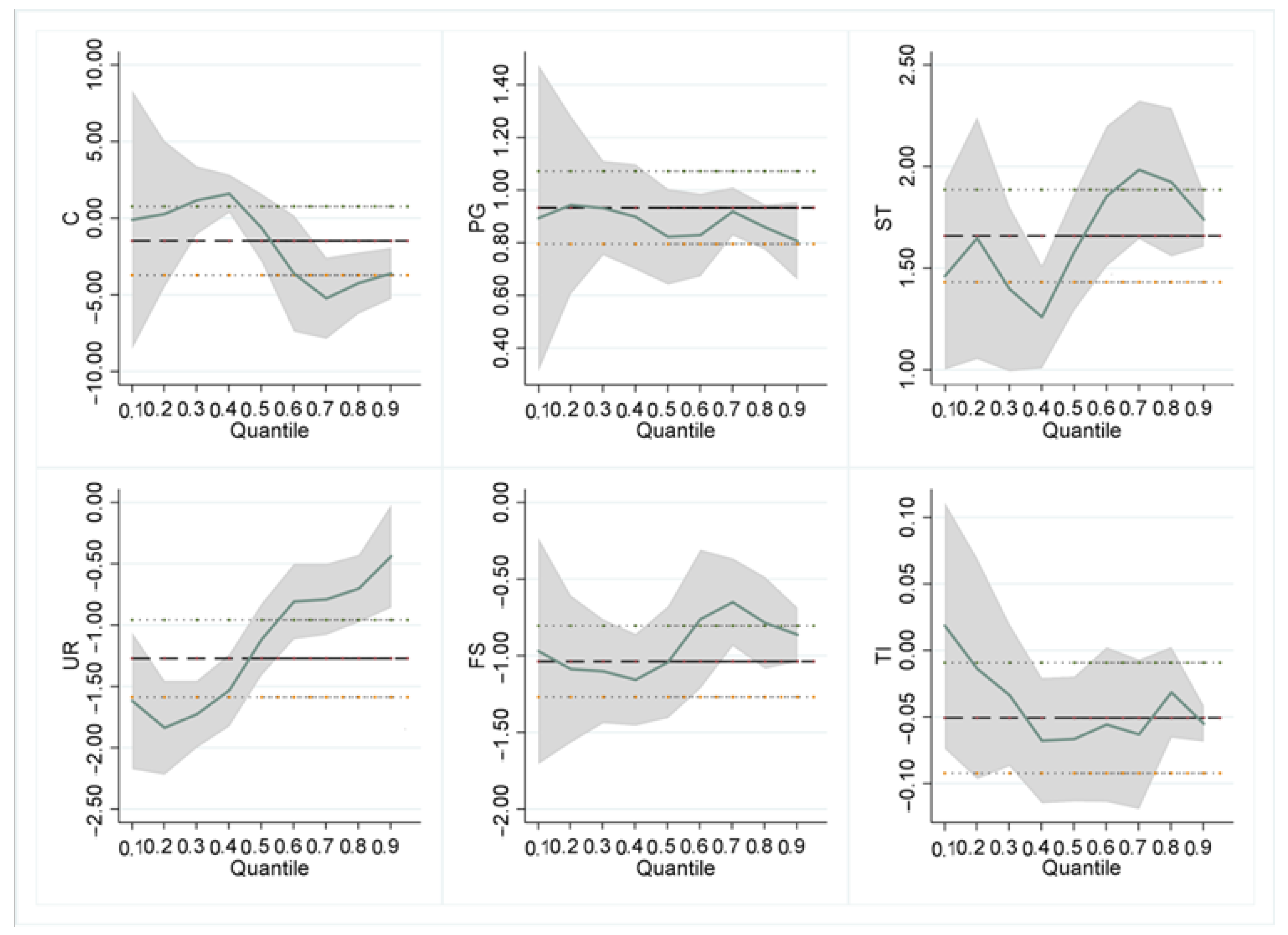
4.2. Results and Discussion of Quantile Regression

The quantile regression results based on Equation (1) are shown in

Table 5. Quantile regression results.

Variables	OLS	Quantile Statistics
		10th	20th	30th	40th	50th	60th	70th	80th	90th
PG	0.933 (0.000)	0.893 (0.003)	0.943 (0.000)	0.932 (0.000)	0.898 (0.000)	0.823 (0.000)	0.829 (0.000)	0.919 (0.000)	0.859 (0.000)	0.806 (0.000)
ST	1.658 (0.000)	1.460 (0.000)	1.648 (0.000)	1.397 (0.000)	1.260 (0.000)	1.580 (0.000)	1.854 (0.000)	1.984 (0.000)	1.923 (0.000)	1.739 (0.000)
UR	−1.272 (0.000)	−1.618 (0.000)	−1.838 (0.000)	−1.727 (0.000)	−1.532 (0.000)	−1.116 (0.000)	−0.808 (0.000)	−0.790 (0.000)	−0.702 (0.000)	−0.438 (0.016)
FS	−1.036 (0.000)	−0.970 (0.017)	−1.087 (0.000)	−1.101 (0.000)	−1.157 (0.000)	−1.042 (0.000)	−0.762 (0.000)	−0.651 (0.000)	−0.786 (0.000)	−0.863 (0.000)
TI	−0.050 (0.011)	0.019 (0.615)	−0.014 (0.687)	−0.034 (0.236)	−0.068 (0.004)	−0.067 (0.005)	−0.056 (0.055)	−0.063 (0.045)	−0.032 (0.176)	−0.055 (0.000)
C	−1.478 (0.192)	−0.103 (0.982)	0.267 (0.913)	1.163 (0.494)	1.596 (0.235)	−0.639 (0.686)	−3.621 (0.063)	−5.228 (0.000)	−4.230 (0.000)	−3.609 (0.000)

. In this study, the OLS method was initially used for the estimation, and then the quantile regression method was applied to the parameter estimation for each 0.1 quantile from 0.1 to 0.9. Figure 3 shows the change in the elasticity coefficient estimated by quantile regression in the conditional distribution of CE, that is, the change in the influence of all the explanatory variables in the conditional distribution on CE, and the shaded area represents the 95% confidence interval of the parameter estimate. The results obtained by the OLS model in Table 5 are only used as a reference frame, and the coefficients obtained by quantile regression indicate that the influence of the respective variables on CE changes with the increase in CE. For example, for PG, Figure 3 shows that across the entire CE conditional distribution, the elastic coefficient of PG was greater than 0 and the shaded area was also above the zero horizontal line, which indicates that PG had a significant effect on CE at different quantiles; in addition, the positive effect on CE varied with increasing CE.

The elasticity coefficient of per capita disposable income (PG) was positive and significant at all quantiles. This indicates that PG promotes the production of carbon emissions at different CE levels. This may be due to the fact that with the rapid growth of China’s economy, the per capita disposable income of Chinese residents has continued to increase in the past few decades, and the increase in income, the level of consumption, and the upgrade of the consumption structure make it easier for them to buy cars, houses, refrigerators, air conditioners, washing machines, and other high-priced items that emit more carbon dioxide. From the change of the quantile regression coefficient of PG, it can be seen that in low CE areas, the coefficient of PG was slightly larger, which may be due to the faster economic development in these areas and the higher income level of the residents, so the consumption of the expenditure is also relatively large, which in turn increases the generation of carbon emissions.

Both the elastic coefficient and confidence interval of the industrial structure (ST) were above the zero horizontal line, which indicates that ST had a positive and significant effect on CE in the whole CE conditional distribution. Moreover, the effect of ST on CE showed an upward trend with the increase in the quantile, and the greater the CE, the greater the effect. In low CE areas, the added value of the secondary industry was lower than that in high CE areas. There are more heavy industries with high energy consumption in high CE areas, and the development of high carbon industries has caused huge pressure on the environment. Conversely, for low CE regions, where the proportion of primary industries is relatively high and there are fewer energy-intensive industries, industrialization may reduce environmental pressures in these regions. Therefore, industrial transfer can alleviate the environmental pressure brought about by industrialization in low-income areas. In addition, through the change of the quantile regression coefficient of ST, it can be seen that the coefficient of ST had a downward trend in high CE areas, which is because China’s industrial structure will be optimized and upgraded with the development of the economy, especially the service industry. The proportion increases rapidly, thereby alleviating the CE pressure brought by high-carbon industries.

The elasticity coefficient of urbanization level (UR) was negative and significant in all quantiles, which is different from the research of most scholars. For example, Huo et al., believe that urbanization has a positive impact on CO₂ emissions [30]. In this study, UR had an inhibitory effect on carbon emissions. This may be because, on the one hand, when urbanization enters an advanced stage, its impact on the environment will be directly or indirectly reduced. This is because the quality of life of the residents continues to improve, and with the development of urban civilization, the awareness of environmental protection is enhanced. On the other hand, the increase in urbanization has also improved the energy structure, especially the connection of liquefied petroleum gas and power grids, replacing traditional fuels with more compact and modern forms of energy. These modern fuels are more efficient and produce less indoor air pollution than traditional fuels. In addition, from the change of the quantile regression coefficient of UR, it can be seen that the inhibition level of UR on CE gradually weakened from low-carbon areas to high-carbon areas. Studies by some scholars have shown that the carbon dioxide emissions of cities at a higher development stage are lower than those of cities at a lower development stage [31]. This is due to the fact that most of the areas with high levels of urbanization have a high density of building forms and the average living area is smaller. These areas require less energy for heating, lighting, and cooling than suburban or rural areas. The second is that these cities have extensive public transportation systems, making travel greener. However, the level of urbanization in high CE areas is at a relatively low development stage, and its ability to suppress carbon emissions has weakened due to resource consumption during its development.

The elasticity coefficients of mean household size (FS) were negative and significant across all quantiles, suggesting that FS has an inhibitory effect on carbon emissions. This is because the impact of family size on carbon emissions is mainly reflected in the consumption field. Under a certain total population, the larger the family size and the smaller the number of family units, the less household necessities purchased by the family unit, resulting in this phenomenon. The reason is due to the existence of scale effects within the family. For example, Underwood believes that due to the existence of economies of scale among households, when adding family members, the increase in carbon dioxide emissions is not proportional to the size of the family [32]. From the change of the quantile regression coefficient of FS, it can be seen that the inhibitory ability of FS on CE was stronger in the low CE area than in the high CE area. This may be due to the higher level of urbanization in the low CE areas, and thus the higher population density and the relatively larger family size.

The effect of the technological innovation level (TI) on CE was only positive at the 0.1 quantile, and negative and significant at other quantiles. This indicated that TI played a promoting effect on CE first, and then played a suppressing effect with the increase in CE. This is because the level of technological innovation improves the efficiency of total factor productivity and also improves the efficiency of energy utilization, thereby reducing energy consumption and carbon emissions. When CE was less than 0.2 quantile, the level of scientific and technological innovation had a slight promotion effect on carbon emissions. This is mainly because people in low CE regions have higher energy demands, and improvements in energy efficiency may lead to more energy consumption (also known as the rebound effect of energy), offsetting some of the expected energy savings from energy efficiency improvements. When CE was in the range of 0.2–0.9 quantiles, the inhibitory effect of the level of technological innovation showed an upward trend. This is because in high CE regions, the potential for innovation levels is greater and there is more room for technology dissemination. In addition, due to the innovation and absorption of late-stage technologies, the resulting technological progress has a gradually increasing impact on CE, thereby obtaining a cumulative effect.

5. Conclusions and Suggestions

Using the panel data of 30 provinces and cities in China from 2000 to 2018, this study analyzed the impact of per capita disposable income, urbanization level, industrial structure, scientific and technological innovation level, and average household size on China’s carbon emissions based on a STIRPAT expansion model. Empirical results for the different determinants of carbon emissions were then presented by panel quantile regression, and the heterogeneous effects of each determinant between low and high quantiles were illustrated. The empirical results showed that per capita disposable income had a positive impact on carbon emissions. Household consumption largely contributed to this positive effect. In addition, due to the characteristics of the country’s economic development, the industrial structure had a greater positive impact on carbon emissions. It is worth noting that the level of urbanization had a significant inhibitory effect on carbon emissions, which was caused by the enhancement of the residents’ awareness of environmental protection and the improvement of the urban energy structure. The average household size had an inhibitory effect on carbon emissions due to scale effects. The improvement of the scientific and technological innovation level had a good effect on reducing carbon emissions. More importantly, the 10th to 90th quantiles of each factor had different effects on emissions at different levels, indicating that regions are moving towards specific emission paths as society develops, rather than tending to the same one path.

Based on the above empirical analysis, this study gives the following policy implications. The government has increased the propaganda of energy conservation and emission reduction, encouraged consumers to use low-carbon products, advocated green consumption habits and living habits, and provided certain financial subsidies for some green behaviors, so as to guide consumers to change from traditional consumption to green consumption, and to adjust and optimize the industrial structure and vigorously develop the tertiary industry. Although the average annual growth rate of carbon emissions in the industrial sector has been declining in the past ten years, due to the large base of carbon emissions brought by industry, it is urgent to formulate and implement effective industrial policies to realize the greening of the country’s industrial structure as soon as possible. For a long time, urbanization will remain the top priority of the government’s work. Provinces and cities should also speed up the construction of urbanization. Although a certain amount of carbon emissions may be generated in the process of urbanization, as urbanization enters an advanced stage, carbon emissions will be suppressed to some extent. Moreover, different cities can develop low-carbon industries with local characteristics and can integrate low carbon into the development process of cities. According to the impact of household size on carbon emissions, when formulating population-related policies, it is possible to appropriately guide the increase in household size level, so as to realize the energy saving and emission reduction in residents in their living consumption. In terms of technological innovation and development, since the low-carbon technologies in low CE regions are still at a low level and the inhibition of carbon emissions is still weak, more and sufficient resources can be used for technological innovation in high CE regions, and then the results can be used in in low CE areas. Second, technologies can be developed independently, but at the same time it is important to learn advanced technologies from others, so it is necessary to introduce and assimilate technologies, thereby acquiring new technologies to accelerate mitigation goals.

References

1. Zhang, C.; Lin, Y. Panel estimation for urbanization, energy consumption and CO2 emissions: A regional analysis in China. Energy Policy 2012, 49, 488–498. [Google Scholar] [CrossRef]
2. Meng, L.; Guo, J.E.; Chai, J.; Zhang, Z. China’s regional CO2 emissions: Characteristics, inter-regional transfer and emission reduction policies. Energy Policy 2011, 39, 6136–6144. [Google Scholar] [CrossRef]
3. Wang, Y.; Wang, L.; Liu, H.; Wang, Y. The Robust Causal Relationships among Domestic Tourism Demand, Carbon Emissions, and Economic Growth in China. SAGE Open 2021, 11, 21582440211054478. [Google Scholar] [CrossRef]
4. Sirag, A.; Matemilola, B.T.; Law, S.H.; Bany-Ariffin, A.N. Does environmental Kuznets curve hypothesis exist? Evidence from dynamic panel threshold. J. Environ. Econ. Policy 2018, 7, 145–165. [Google Scholar] [CrossRef]
5. Nasir, M.; Rehman, F.U. Environmental Kuznets Curve for carbon emissions in Pakistan: An empirical investigation. Energy Policy 2011, 39, 1857–1864. [Google Scholar] [CrossRef]
6. Ozturk, I.; Acaravci, A. The long-run and causal analysis of energy, growth, openness and financial development on carbon emissions in Turkey. Energy Econ. 2013, 36, 262–267. [Google Scholar] [CrossRef]
7. Jorgenson, A.K.; Clark, B. Assessing the temporal stability of the population/environment relationship in comparative perspective: A cross-national panel study of carbon dioxide emissions, 1960–2005. Popul. Environ. 2010, 32, 27–41. [Google Scholar] [CrossRef]
8. Song, M.; Wu, J.; Song, M.; Zhang, L.; Zhu, Y. Spatiotemporal regularity and spillover effects of carbon emission intensity in China′s Bohai Economic Rim. Sci. Total Environ. 2020, 740, 140184. [Google Scholar] [CrossRef]
9. Qi, X.; Han, Y.; Kou, P. Population urbanization, trade openness and carbon emissions: An empirical analysis based on China. Air Qual. Atmos. Health 2020, 13, 1–10. [Google Scholar] [CrossRef]
10. Zhu, H.M.; You, W.H.; Zeng, Z.F. Urbanization and CO2 emissions: A semi-parametric panel data analysis. Econ. Lett. 2012, 117, 848–850. [Google Scholar] [CrossRef]
11. Al-Mulali, U.; Sab, C.N.B.C.; Fereidouni, H.G. Exploring the bi-directional long run relationship between urbanization, energy consumption, and carbon dioxide emission. Energy 2012, 46, 156–167. [Google Scholar] [CrossRef]
12. Poumanyvong, P.; Kaneko, S. Does urbanization lead to less energy use and lower CO2 emissions? A cross-country analysis. Ecol. Econ. 2010, 70, 434–444. [Google Scholar] [CrossRef]
13. Chuai, X.; Feng, J. High resolution carbon emissions simulation and spatial heterogeneity analysis based on big data in Nanjing City, China. Sci. Total Environ. 2019, 686, 828–837. [Google Scholar] [CrossRef] [PubMed]
14. Robert, J.R.; Shanshan, W.U. Industrial activity and the environment in China: An industry-level analysis. China Econ. Rev. 2008, 19, 393–408. [Google Scholar]
15. York, R.; Rosa, E.A.; Dietz, T. STIRPAT, IPAT and ImPACT: Analytic tools for unpacking the driving forces of environmental impacts. Ecol. Econ. 2003, 46, 351–365. [Google Scholar] [CrossRef]
16. Ota, T.; Kakinaka, M.; Kotani, K. Demographic effects on residential electricity and city gas consumption in the aging society of Japan. Energy Policy 2018, 115, 503–513. [Google Scholar] [CrossRef] [Green Version]
17. Martínez-Zarzoso, I.; Maruotti, A. The Impact of Urbanization on CO2 Emissions: Evidence from Developing Countries. Ecol. Econ. 2011, 70, 1344–1353. [Google Scholar] [CrossRef] [Green Version]
18. Shahbaz, M.; Loganathan, N.; Sbia, R.; Afza, T. The effect of urbanization, affluence and trade openness on energy consumption: A time series analysis in Malaysia. Renew. Sustain. Energy Rev. 2015, 47, 683–693. [Google Scholar] [CrossRef] [Green Version]
19. Chen, Q.; Mao, Y.; Morrison, A.M. Impacts of Environmental Regulations on Tourism Carbon Emissions. International. J. Environ. Res. Public Health 2021, 18, 12850. [Google Scholar] [CrossRef]
20. Chen, X.; Chen, Z. Can Green Finance Development Reduce Carbon Emissions? Empirical Evidence from 30 Chinese Provinces. Sustainability 2021, 13, 12137. [Google Scholar] [CrossRef]
21. Tiba, S.; Belaid, F. The pollution concern in the era of globalization: Do the contribution of foreign direct investment and trade openness matter? Energy Econ. 2020, 92, 104966. [Google Scholar] [CrossRef]
22. Bassett, K.G. Regression Quantiles. Econometrica 1978, 46, 33–50. [Google Scholar]
23. Kato, K.; Galvao, A.F.; Montes-Rojas, G.V. Asymptotics for panel quantile regression models with individual effects. J. Econom. 2012, 170, 76–91. [Google Scholar] [CrossRef] [Green Version]
24. Koenker, R. Quantile regression for longitudinal data. J. Multivar. Anal. 2004, 91, 74–89. [Google Scholar] [CrossRef] [Green Version]
25. Lamarche, C. Measuring the incentives to learn in Colombia using new quantile regression approaches. J. Dev. Econ. 2011, 96, 278–288. [Google Scholar] [CrossRef]
26. Damette, O.; Delacote, P. On the economic factors of deforestation: What can we learn from quantile analysis? Econ. Model. 2012, 29, 2427–2434. [Google Scholar] [CrossRef] [Green Version]
27. Maddala, G.S.; Wu, S. A Comparative Study of Unit Root Tests with Panel Data and a New Simple Test. Oxf. Bull. Econ. Stat. 1999, 61, 631–652. [Google Scholar] [CrossRef]
28. Pedroni, P. Critical Values for Cointegration Tests in Heterogeneous Panels with Multiple Regressors. Oxf. Bull. Econ. Stat. 1999, 61, 653–670. [Google Scholar] [CrossRef]
29. Kao, C. Spurious regression and residual-based tests for cointegration in panel data. J. Econom. 2004, 90, 1–44. [Google Scholar] [CrossRef]
30. Huo, T.; Cao, R.; Du, H.; Zhang, J.; Cai, W.; Liu, B. Nonlinear influence of urbanization on China′s urban residential building carbon emissions: New evidence from panel threshold model. Sci. Total Environ. 2021, 772, 145058. [Google Scholar] [CrossRef]
31. Dhakal, S.; Kaneko, S.; Imura, H. An analysis on driving factors for CO2 emissions from energy use in Tokyo and Seoul by factor decomposition method. Environ. Syst. Res. 2002, 30, 295–303. [Google Scholar] [CrossRef] [Green Version]
32. Underwood, A.; Fremstad, A. Does sharing backfire? A decomposition of household and urban economies in CO2 emissions. Energy Policy 2018, 123, 404–413. [Google Scholar] [CrossRef]
Figure 1. Histogram of CE variables.
Sustainability 14 07791 g001
Figure 2. National carbon emissions from 2000 to 2018.
Sustainability 14 07791 g002
Figure 3. Variation of quantile regression coefficient. (The area between the upper and lower two different colors is the confidence interval.)
Sustainability 14 07791 g003