Abstract
The interest in the use of mathematical models for the simulation of hydrological processes has largely increased especially in the prediction of runoff. It is the subject of extreme research among engineers and hydrologists. This study attempts to develop a simple conceptual model that reflects the features of the arid environment where the availability of hydrological data is scarce. The model simulates an hourly streamflow hydrograph and the peak flow rate for any given storm. Hourly rainfall, potential evapotranspiration, and streamflow record are the significant input prerequisites for this model. The proposed model applied two (2) different hydrologic routing techniques: the time area curve method (wetted area of the catchment) and the Muskingum method (catchment main channel). The model was calibrated and analyzed based on the data collected from arid catchment in the center of Jordan. The model performance was evaluated via goodness of fit. The simulation of the proposed model fits both (a) observed and simulated streamflow and (b) observed and simulated peak flow rate. The model has the potential to be used for peak discharges’ prediction during a storm period. The modeling approach described in this study has to be tested in additional catchments with appropriate data length in order to attain reliable model parameters.
1. Introduction
Flood forecasting studies particularly in arid areas have become of great importance in water resources engineering and water science research [1]. Compared with a basic economic system, modern societies and new cities are less capable of coping with natural disasters, such as flood [2]. Mathematical conceptual and flood routing hydrological models are developed for a better understanding of the surface runoff formation originating from a complex watershed.
The beginning of an extensive modelling on rainfall–runoff at large numbers of watershed was reported in the latter part of the 19th century. It was due to urgent applications by engineers working in the designs of urban sewers, flood control structures, and dam spillways. The design on discharge is quiet challenging. In the sixties of the last century, conceptual approaches to rainfall–runoff modeling were taken into consideration in looking for a better interpretation of hydrological processes.
The linear store conceptual approach as a delay mechanism in the computational rainfall–runoff relationship has been introduced [3]. This approach has become an evolution in conceptual rainfall–runoff models. Meanwhile, the “soil moisture accounting” model has a structure of interconnected storage. In comparison with black-box models, linear stores and soil moisture accounting models are more complicated with no direct physical explanation.
Mroczkowski et al. defined a conceptual model as a model that requires at least one of its parameters to be calibrated [4]. However, conceptual models have limitation. Conceptual models have no simulation on other hydrological processes, such as infiltration and groundwater level, and they mostly produce a single output (i.e., streamflow). Examples of conceptual models are Stanford [5], HBV (Sweden) [6], TANK (Japan) [7], Modhydrolog (Australia) [8], Xianjiang (China) [9], and Arno (Italy) [10].
Conceptual models provide short and long forecasts of runoff or any other variables. The magnitude of extreme events can also be predicted with conceptual models, which are important for water management. The approach for estimating extreme flood events by fitting extreme value distribution to the maximum values of observation has been widely criticized [11,12] since distribution functions have to be extended out of the probability range obtained from available records. Therefore, the modeling approach is a better alternative to distribution fitting. Nearly all conceptual models can produce compatible and dependable results. They appear to be very suitable because they require less data and simple structures. Moreover, they are less expensive and user friendly [1,13,14,15,16,17,18,19,20].
In real-world applications that do not require an internal catchment process, the conceptual model is known to provide a good estimate of runoff at the catchment outlet, so a conceptual model with a small number of parameters is the best approach. Meanwhile, physically based distributed models provide the best option to model internal catchment processes [21], but field observations, data preparation, and parameter calibration are very expensive [22].
Several conceptual models have been used for flood estimation in arid and semiarid regions. The IHACRES (Identification of unit Hydrographs and Component flows from Rainfall, Evaporation, and Streamflow data) conceptual model was found to be successful for the application in the Wadi Dhuliel arid catchment, northeast Jordan. The model performance showed a good agreement between observed and simulated streamflow when running the model on a discrete event basis [23]. A study was conducted in Iran to compare the performance of the IHACRES conceptual model with a complex watershed model, SWAT. The study revealed that both models had acceptable performances in the semiarid and semihumid watersheds. Nevertheless, the performance of SWAT was better than that of IHACRES specifically in the arid watershed [24]. The GR4H (in French, Génie Rural à 4 paramétres Horaires) rainfall–runoff model was reported to be more reliable for the simulation of wet years, and it was applied for watersheds that are unaffected by land cover changes [25].
Many conceptual models have been developed, but only a limited number have been found suitable for the simulation of runoff in arid regions. In this study, a simple modelling approach is proposed that is based on a simple conceptualization of hydrological processes within a watershed. Stress on water resources in arid regions is alarming. Therefore, the development of water resources management approaches, such as a conceptual rainfall–runoff model, is highly in demand. This model can bridge the gap between complex and spatially distributed models. These types of models require intensive hydrological and climatological data and simple empirical models that are less precise in predicting runoff. Simple modelling approaches proposed in this study offer a number of advantages in the management of water resources, especially in data-scarce regions.
The aim of the present study is to develop a simple rainfall–runoff modelling approach with simple conceptual structures and with more parsimonious parametrizations. The validity of this simple modeling approach in predicting the peak flow rate in arid catchments was included.
2. Materials and Methods
2.1. Hydrologic Data
The model was applied to the Wadi Walla arid catchment, Jordan. This catchment is located at 60 km southwest of Amman City; the location of this catchment is shown in Figure 1. The 1770 km2 area mainly consists of elevated land. The Wadi Wala catchment is classified as arid because of low rainfall in most of the catchment in winter and high temperature in summer [21]. The mean annual rainfall over the catchment is approximately 300 mm, and the mean temperature range is within 150 °C.
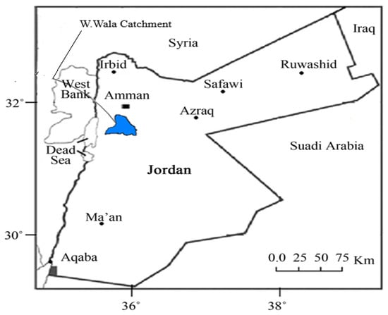
Figure 1.
Location map of the Wadi Walla catchment.
2.1.1. Soil Condition
The soil in the Wadi Wala catchment adjacent to the western hills ranges from red to yellow Mediterranean soil, whereas grey soils are predominant on the eastern side of the catchment. The runoff characteristics are greatly influenced by the predominant type of soil due to the variation in infiltration capacity [22].
To investigate the dominant soil texture in the Wadi Wala catchment, a soil map of the Wadi Wala catchment was obtained and carefully inspected. Based on the information provided by the soil map, it can be concluded that the dominant soil texture at the Wadi Wala catchment may be considered as silty clay loam. This texture was assumed to be uniform in the upper soil layer of the catchment. The soil may also be considered as isotropic. The detailed soil characteristic classification was based on Rawls [23].
2.1.2. Evaluation and Analysis of Available Data
The hydrological and meteorological data for the Wadi Wala catchment were collected from unpublished files of the Water Authority of Jordan (WAJ). Hourly rainfall data were recorded from 1990 to 2001 at three different recording rainfall stations.
2.2. Model Structure
The presented model in this study was developed based on the analysis of previously published reports. The general structure for the proposed model is shown in Figure 2.
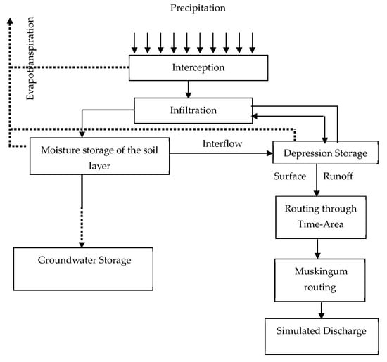
Figure 2.
Schematic diagram of the proposed model structure.
The model was established on the water balance principles according to Equation (1).
where:
- Ra = the total surface runoff depth (mm);
- Pa = the total precipitation depth (mm);
- Fa = the total infiltration depth (mm);
- Sin = the interception storage depth (mm);
- PET = the potential evapotranspiration depth (mm);
- Ds = the surface depression storage depth (mm).
2.2.1. Model Components and Conceptualization
The proposed model is made up of a series of computational routines for each process in the hydrologic cycle. The main components for the model were precipitation, interception, surface depression storage, infiltration, subsurface flow (in the past, it was called hypodermic flow; relatively, it is an impermeable shallow layer), deep percolation (water percolates into the deeper layers of the soil), streamflow recession, and catchment routing.
The falling precipitation is partly intercepted by vegetation. The amount of interception depends on the canopy density and types of vegetative plants covering the catchment area.
The model simulates interception using an equation suggested by Fleming [24], which is expressed by Equation (2):
where ∆Sin is the difference in interception storage, when the maximum storage capacity is larger than the current interception. Pd refers to the precipitation depth per unit area of the catchment. Dc refers to the canopy density, and Ein is the loss per unit area from the interception due to evaporation and transpiration. Interception storage Sin will be depleted by evapotranspiration PET. Excess water (throughfall) flows to the ground surface upon meeting the requirement of interception storage. Throughfall was estimated using Equation (3):
Tin indicates throughfall upon exceeding the interception storage capacity. Sin(t−1) refers to interception storage at time taken (t − 1). Smax refers to the maximum interception storage capacity. Equation (4) describes the condition of throughfall and rainwater reaching the ground surface and infiltrating into the soil [25].
where:
- f = the infiltration capacity rate (mm/h);
- Sa = the available storage capacity depth from the surface (mm).
At the beginning of infiltration, Sa is usually at its initial value Sai (Sai is the first model parameter), a and n are the intercept and slope, respectively, of an algorithmic plot of the quantity (f − fc) versus Sa (a and n are the second and third model parameters).
fc = constant rate of infiltration (mm/h) (fc is the fourth model parameter).
Whenever the rate of water hits the ground surface at a rate larger than the infiltration capacity, the water in excess of the infiltration capacity will be added to the surface depression storage Ds. At the same time, this storage will be depleted by evaporation (Er) and infiltration (Fa). Depression storage is depleted by evapotranspiration PET and direct infiltration to the soil moisture storage SMS. Depression storage has a finite capacity Dmax (Dmax is the fifth model parameter), and when that capacity is exceeded, direct runoff DRO occurs. DRO is computed in agreement with Equations (5) and (6), which are given as follows:
where:
- DRO = the direct surface runoff (mm);
- Sci = the capacity depth of inflow into interception storage (mm) for each time increment;
- Dc = the capacity depth of inflow into surface depression storage for each time increment.
The storage of soil moisture is supplemented by infiltration and diminished by evapotranspiration. The percolation and subsurface flow will commence after the storage of soil moisture reaches its threshold (field capacity, FC). The model assumed that percolation is taking place at a rate smaller than fc. Subsurface flow is estimated according to Equations (7) and (8):
where Gravw is gravitational water in mm, SSF is subsurface flow in mm for each time increment, SW is the water sustained above field capacity, and Sc is the coefficient of subsurface flow (Sc is the sixth model parameter).
Subsurface flow SSF continuously augments surface depression storage. If the latter exceeds its threshold, surface runoff occurs. The recovery of moisture storage capacity between the periods of rain may be estimated by Equation (9):
where:
- PET = the potential evapotranspiration rate (mm/h);
- PER = the percolation (mm);
- SSF = the subsurface flow (mm);
- Δt = the time increment (h);
- t = the time index.
2.2.2. Streamflow Recession
The recession or receding limb of the streamflow hydrograph is that part between time to peak and time base. It can be defined as the gradual depletion of discharge during periods with little or no precipitation, and it is logarithmic in nature. The recession curve represents withdrawal from storage within the basin. The general equation used to describe the recession curve can be given by Equation (10):
where:
- Q0 = the flow at any time in cumecs;
- Qt = the flow one time unit later in cumecs;
- Kr = the recession constant (Kr, the seventh model parameter).
2.2.3. Catchment Routing
Catchment routing is performed using two different approaches; the first is time–area curve routing, and the second is catchment channel flow routing. The time–area method of hydrologic catchment routing transforms an effective storm hyetograph into a runoff hydrograph. The method accounts for translation only and does not include storage. The time–area curve method originates from the concept of time–area histogram. The relative delay time or the time of concentration is estimated using the Kirpich equation, which is given by Equation (11):
where:
- Tc = time of concentration in hours;
- Lc = channel reach length (m);
- So = mean slope of channel reach.
The general nonlinear time–area curve relation for the catchment is given by Equation (12):
where:
- A = the catchment area (km2), starting point from the Wadi outlet to the most remote point of surface runoff movement):
- c & d = regression coefficients.
Equation (12) is used to compute the accumulated wetted catchment area and its corresponding time of concentration. Each subarea is then multiplied by rainfall excess array resulting from catchment water balance. The result will be the surface runoff at the outlet of the wetted area. This yields a set of linear equations expressed in matrix form, as shown in Equations (13) and (14). The number of ordinates in rainfall excess is a unit hydrograph. A unit hydrograph is a hydrograph of surface runoff resulting from a relatively short, intense rain, called a unit storm (flow of runoff, m3/sec versus time, hour). It can predict the flood peak discharges and determines the direct runoff response to rainfall. Both gauged and ungauged basins as well as basin characteristics (drainage area, slope, etc.) are considered in this method. The analysis method of unit hydrograph commonly employs the summation curve (S-curve), instantaneous unit hydrograph, and synthetic unit hydrograph [26]:
or
where:
- Re = the rainfall excess array (mm/h);
- Aw = the watershed wetted subarea column vector (km2);
- q = the wetted area outflow discharge column vector;
- Nr = the number of ordinates of rainfall excess;
- M = the number of wetted subarea;
- J = the number of wetted area outflow discharge.
The catchment channel flow routing is performed by the model using the Muskingum method, which is mostly used for handling a variable discharge–storage relationship. The common storage function used in the Muskingum method is given by Equation (15):
where:
- k = the travel time of the flood wave through the channel reach in an hour (k is the eighth model parameter);
- x = the weighing factor ranging from 0 to 0.5 (x is the ninth model parameter. The model performs channel routing using the Muskingum routing equations (Equations (16)–(19)):
2.2.4. Lag Time and Wetted Area Approach
Most hydrologic models require watershed characteristics that reflect the timing of runoff. In this study, a simple definition of lag time is adopted, that is, “the time delay between the beginning of the rain and the runoff commencement at the outlet of the catchment”.
Generally, lag time is affected by watershed and rainstorm parameters. The lag time of large and medium catchments TL is the sum of three lag times; the soil absorbed basin time Tb, which is the time from the start of the storm till the surface runoff occurs on the wetted area; the wetted area travel time Ta, which is the time from the start of runoff in the wetted area till the outlet of the wetted area; and the travel time Tv, which is the time from the wetted area outlet till the outlet of catchment or gauging station. This can be expressed by Equation (20):
The travel time for the catchment’ main channel could then be obtained using Equation (20), which is expressed by:
The wetted area is usually determined from fieldwork. However, when this is not available as the condition of the catchment under study, the number of wetted areas NA is considered as a parameter to be determined by using optimization technique (NA is the tenth model parameter). The wetted subareas can then be obtained with the help of Equation (12). The resulting effective rainfall or surface runoff depth Re and all wetted subareas are routed using Equations (13) and (14) to obtain the surface runoff rate at the outlet of the wetted area for each applied storm. The model utilizes the difference in base time of the observed and simulated runoff hydrograph, which is called (recession time) to compute the remainder simulated flow rate. In case the difference is smaller than or equal to zero, the simulated base time is considered equal to its measured value.
The time lag from the wetted area outlet somewhere inside the catchment to the catchment outlet is computed using Equation (21). This time is called travel time Tv, which is divided equally into a number of cascade reaches; the outflow from the first reach is taking as inflow to the next reach and so on. The flow through these reaches is routed by applying the Muskingum method for hydrologic flow routing. Equations (16)–(19) are all used in routing procedures. The parameters x and k in these equations are obtained through optimization technique.
2.2.5. Catchment Area Parceling Condition
The catchment area is divided into subareas by isochrones. Then for each point, the distance to the outlet of the catchment is tabulated, and the slope of this distance is determined. The travel time for each point is calculated with the help of Equation (11). The time–area curve equation is established using a general regression method. The evolved equation with its fitted curve is shown in Figure 3.
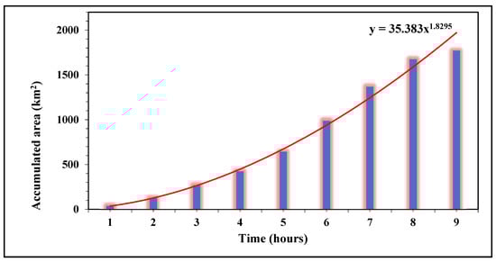
Figure 3.
Accumulated time area curve for the Wadi Wala catchment.
2.3. Model Calibration
The parameters of a watershed model cannot, in general, be determined directly from the physical characteristics of the catchment, and hence, the parameter values must be estimated by calibration against observed data. Calibration is the process of estimating model parameters; the parameter values are continuously adjusted until the values of model outputs agree with actual outputs. Calibration begins with a first estimate of model parameters. By using the observed meteorological inputs, the hourly or daily streamflow predicted by the model is compared with the observed hourly or daily streamflow. Appropriate parameters are adjusted until the predicted hourly or daily streamflow is acceptably close to the observed values.
The major aim of calibration in hydrological modeling is to reduce the variation between observed and simulated flows. This variation is usually represented via a mathematical function.
In this study, a least-square objective function is used for fitting the parameters of the proposed model. The least-square objective function is given in Equation (22):
where:
- OF (LS) = a least-square objective function;
- Qobsi = the observed flow on any hour i;
- Qsimi = the simulated flow on any hour i;
- N = the number of record observations.
Calibration begins with a first estimate of model parameters. By using the observed meteorological inputs, the hourly streamflow predicted by the model is compared with the observed hourly streamflow. Appropriate parameters are adjusted until the predicted streamflow is acceptably close to the observed values. In this study, the shuffle complex evolution global optimization method [27] is used for the calibration of the model parameters. Some of the input requirements for this optimization method are as follows: maximum number of trials allowed, number of shuffling loops in which the criterion must improve by the specified percentage, percentage by which the criterion value must change in the specified number of shuffling loops, number of complexes used for optimization search, random seed used in optimization search, and initial estimates of the parameters to be optimized with their upper and lower bounds.
There are three (3) criteria applied in the SCE-UA (shuffled complex evolution optimization approach) for the termination of the model. The criteria are: (a) the number of shuffling iterations is greater than 19, (b) the change in objective function and parameters values is less than 0.0001, and (c) the number of iterations is greater than 90,000 iterations.
2.4. Model Validation
The viability of any model is determined mainly by its capability to reproduce the hydrological processes in the catchment under study accurately and efficiently. To accomplish this task, much hydrological data are needed to determine the optimal parameters for the applied model. Additional standard procedures are required for the validation of hydrological modelling. These procedures are called model validation or verification.
In this study, the collected hydrological data are divided into two parts; each part consists of a number of storm events. The model is tested by using the optimized parameters obtained from the first part to evaluate the data of the second part except the two important parameters, Sai and NA (which are dependent on catchment initial soil moisture condition and storm event characteristics). Sai and NA are optimized individually for each storm.
Performance Evaluation of the Proposed Model
Four performance criteria are used in this study [28,29,30]. The coefficient of efficiency is the dimensionless expression as given in Equation (23):
where:
- f (Qobsi) = the observed streamflow;
- f (Qsimi) = the simulated streamflow over the calibration period;
- N = the number of record observations.
The coefficient of determination r2 indicates the level of agreement between observed and simulated hydrographs. The coefficient of determination r2 is given by Equation (24):
The IVF is the volumetric fit index given by Equation (25). It is the ratio of the total simulated volume (Vsimi) to the total observed volume (Vobsi):
The relative error of the maximum peak flow RE is defined by Equation (26):
where:
- (Qp)obs = the observed peak;
- (Qp)sim = the estimated peak.
3. Results and Discussion
Generally, simulation results show a good match between observed and simulated hydrographs in all modeling situations. Coefficient of efficiency R2 and coefficient of determination r2 are provided with all figures to assess the performance of the simulation process. Storm data were used as input into continuous calibration so that the resulting optimal set of parameters will give the average set of all events. Figure 4 shows both observed and optimized hydrographs with their rainstorm’s hyetograph. For all storms, the values of R2 range from 76% to 98%, whereas r2 ranges from 77% to 98%. Similarly, Figure 5 illustrates a comparison of the validation process for the observed and simulated hydrographs. The R2 values for all storms used in validation ranges from 80% to 92%. Similarly, r2 values for the same storm ranges from 87% to 95%.
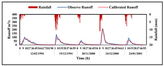
Figure 4.
Observe and calibrated hydrographs of the Wadi Wala catchment.
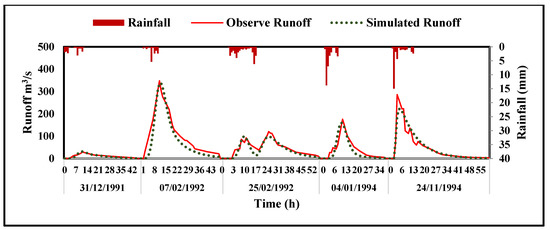
Figure 5.
Observe and simulated hydrographs of the Wadi Wala catchment.
The optimized parameters for the proposed model are all provided in Table 1; the parameters Sai and NA are optimized individually for each storm since they are highly dependent on the storm characteristics, which are different from one storm to other. The values are provided as an average for all the storms.

Table 1.
Optimum parameters of the proposed model along with their upper and lower bounds.
Table 2 shows a comparison between some features of observed and simulated hydrographs for the test catchment. These characteristics, such as time to peak, peak flow, runoff volume, and runoff coefficients, are all presented along with the performance evaluation indices IVE and RE to provide guidance to understand the quality of model simulation. The table shows remarkable coincidence between the characteristics of observed and optimized or simulated hydrographs. The values of IVE for all storms indicate that the volumetric fit between all observed and simulated storms is satisfactory. RE values indicate also that the model simulates peak flow rate equally well.
Table 2.
Some characteristics of observed and simulated hydrographs for the Wala catchment.
Table 3 illustrate the effects of Sai and NA on the runoff coefficient and peak flow rate. A higher peak flow results in a smaller value of Sai and a higher value of NA. The lower Sai value indicates that initial losses are minor, and most of the storm rainfall depth is directly converted into runoff depth. The higher value of NA will further increase the flow peak because a larger area will contribute to the developed peak flow rate. It is worthy to mention that the peak flow rate is affected largely by storm characteristics, such as storm intensity and duration, as most flash floods that usually occur at arid and semiarid catchments essentially emerge due to the occurrence of a massive rain event of high intensity and long or short duration. The runoff coefficient C for all storms falls between 0.039 and 0.45, which fall within the range that is commonly found in most arid and semiarid catchments. Figure 6 shows a closer match between the simulated and measured peak values, which reflect the model capability to produce the peak runoff hydrograph at a reasonable accuracy within the watershed.
Table 3.
Effects of Sai and NA on runoff coefficient and peak flow rate.
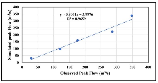
Figure 6.
Observe and simulated peak flow rate on the Wadi Wala catchment.
Model sensitivity analysis (PSA) is performed to reveal how parameter changes affect model performance, which is an important step in model uncertainty analysis. The results of the sensitivity analysis are all listed in Table 4 and Table 5 for a selected storm event of the Wadi Wala catchment. The importance of each optimal parameter is investigated in the light of sensitivity measures SEN.
Table 4.
Sensitivity analysis of the proposed model parameters (storm event: 19 December 1994).
Table 5.
Sensitivity analysis of the proposed model parameters (storm event: 19/12/1994).
The diagnosis of the optimal model parameters is thoroughly discussed and presented as follows for the storm event of 19 December 1994:
Holtan’s equation parameters (a, n and fc) are considered sensitive parameters. This is clearly shown in Table 4 and Table 5. The parameter “a” has a value of SEN 36.8 for a 10% increase in optimal parameter value and 38.4 for a 10% decrease in optimal parameter value, which means that a 10% increase in the optimized value of “a” will result in 36.8% increase in objective function. Similarly, a 10% decrease in the optimized value of “a” will result in a 38.4% decrease in objective function. The parameter “n” has a SEN value of 57.8. This could be explained as for a 10% increase in the value of “n”, there will be a 57.8% increase in objective function. When the value of “n” decreases by 10%, the corresponding decrease in objective function is 55.8%. The parameter “fc” has a SEN value of 5.9, which means that a 10% increase in the value of “fc” will result in a 5.9% increase in objective function, while a 10% decrease in “fc” will decrease the value of the parameter to a value less than its lower constraint. Since the optimal value of “fc” is equal to the parameter’s lower bound, the SEN value for a 10% decrease in its optimal value is not investigated. The aforementioned analysis reveals that the parameters “a” and “n” are more sensitive than the parameter “fc”. Therefore, these parameters should be optimized properly in all modeling conditions.
The parameters (a, n, and fc) depend on the type of surface soil profile and the antecedent soil moisture condition. These three parameters significantly influence the value of infiltration capacity. Infiltration capacity is directly related to the moisture content preserved in the soil at the start of the rain.
In this study, it is found that the parameter fc is taking value equal to its lower constraint, and that the estimated infiltration rate does not reach its final steady rate fc. This may be attributed to the prevailing soil type at the catchment under study (silty clay loam), which is considered heavy soil and usually having a lower infiltration rate. The other reason is the nature of the storm rainfall at arid and semiarid catchments, which is usually marked by short duration and high intensity.
The values of the infiltration parameters “a” and “n” are somewhat apart. This difference can be neglected because any increase or decrease in the value of the parameter “n” is compensated by the same amount in the value of the parameter “a” and vice versa.
The maximum depression storage capacity Dmax is found to be very sensitive; this is clearly shown in Table 4 and Table 5. The SEN values for an increase and decrease in the value of Dmax are 20 and 91, respectively. Generally, the value of Dmax is relatively small and closer to its lower constraints. This low value of Dmax can be attributed to the catchment’s higher relief in its prevailing steep slope. An accurate estimation of Dmax requires that a major field works, and a complete land survey should be performed on the catchment under study.
The initial soil moisture storage capacity Sai is a major parameter involved in several modeling processes. The sensitivity measure SEN for decreasing the parameter value by 10% is very high. This is clearly shown in Table 5. The value of SEN takes as much as 94, which is a very high value. Therefore, Sai must be optimized in all modeling applications.
With a once-over on the values of Sai, one can observe that the majority of the values are closer to the lower constraint of the parameter. In other words, the available soil moisture storage capacity is very limited, and mostly, for all storms, the moisture level at the catchments soil is greater than the field capacity. This low value of Sai is justified by the fact that the time lag between each consecutive storm event is relatively short. This is true since in this study, many storms are neglected due to suspicion that they contained errors.
The interflow coefficient Sc takes value near its lower constraint. The sensitivity measure SEN is equal to zero, which indicates that Sc is an insensitive parameter. Interflow commonly takes place in mountain soils where vegetative cover can produce a layer on the surface characterized by high porosity, but in a relatively bare soil, as the condition in most arid and semiarid catchments, the situation is reversed. Since it is very hard to anticipate the occurrence of interflow in the catchment, the interflow parameter Sc should always be optimized. Sc may be set to a value of zero if a rough estimate of runoff is only needed. It is hard to associate Sc with any watershed characteristics, and its value should always be optimized.
The recession coefficient Kr is important in discrete event modeling. The sensitivity measure SEN is somewhat high. The parameter Kr depends mainly on storm characteristics (intensity, duration, and frequency) and catchment characteristics (such as soil type and catchment relief).
The Muskingum equation parameter “k” (storage time of the reach) is an important parameter when hydrological streamflow routing is required. The sensitivity measure SEN for this parameter is relatively small.
The above analysis reveals that Sai is the most sensitive model parameter, and therefore, care should be taken when optimizing this parameter; the initial soil moisture storage should be assessed carefully in the catchment before conducting the calibration.
4. Conclusions
The simplified conceptual modeling approach just like the one adopted in this study is capable of providing satisfactory simulation for the streamflow and peak flow rate. It is expected that the proposed model will give identical results if it is applied to other catchments, with climatological and hydrological characteristics similar to the test catchment.
The modeling approach proposed in this study is simple, sound, and precise theoretically and practically. It can provide efficient and fast prediction of runoff at arid and semiarid catchments, with limited data. The model might be useful in predicting the peak flow rate and may help in water resources planning and management at arid and semiarid catchments.
A proper selection of objective function that would better suit the type of flow produced from the catchment (i.e., high flow or low flow) could possibly improve the reliability of the streamflow prediction at arid and semiarid catchments, which are mostly characterized as a low-flow yield catchments.
The proposed model is a useful tool for hydrological planning and forecasting, but the model has limitations. In order to obtain reliable results, the model must be calibrated, and the parameters must be adjusted; the calculated runoff is close to observed runoff. A long record of observed runoff data is required for accurate calibration, so the model is largely limited to the extent of available runoff data. It is also increasingly accepted that automatic calibration techniques can actually provide a suboptimal solution. Additionally, due to the interdependence of model parameters, more than one set of parameters can produce equally acceptable results. It has been found that some parameters are sensitive, and careful attention should be taken when optimizing those parameters.
Despite good simulation results obtained by applying the modeling approach presented in this study, there are some errors that might emerge due to imperfect model structure or simplifying assumptions, which may con the validity of model simulation. These errors may possibly emerge due to lack of sufficient hydrological data and unavailability of reliable information on catchment soil physical properties.
In order to obtain reliable model parameters, the modelling approach proposed in this study needs to be tested in other catchments that have relatively sufficient data.
Author Contributions
Conceptualization, A.A.J.G.; methodology, A.A.J.G., T.K., A.M. and S.Y.; software, A.A.J.G.; validation, S.B., T.S.B.A.M. and W.H.M.W.M.; formal analysis, T.K. and D.M.; investigation, A.A.J.G., M.I., S.N.F.M. and N.L.M.K.; resources, A.A.J.G., M.I. and N.L.M.K.; writing—original draft preparation, A.A.J.G., S.B. and T.S.B.A.M.; writing—review and editing, S.H.A.Y., A.A. and N.W.R.; supervision, A.A.J.G.; project administration, A.A.J.G. and S.N.F.M.; funding acquisition, A.A.J.G. All authors have read and agreed to the published version of the manuscript.
Funding
The authors acknowledge the support from the Ministry of Education and the Deanship of Scientific Research, Najran University, Kingdom of Saudi Arabia, under Code Number NU/-/SERC/10/541.
Institutional Review Board Statement
Not applicable.
Informed Consent Statement
Not applicable.
Data Availability Statement
Not applicable.
Acknowledgments
The authors are thankful to the Ministry of Education of the Kingdom of Saudi Arabia; Najran University (Deanship of Scientific Research) for their financial and technical support.
Conflicts of Interest
The authors declare no conflict of interest.
References
- Kan, G.; He, X.; Ding, L.; Li, J.; Liang, K.; Hong, Y. Study on Applicability of Conceptual Hydrological Models for Flood Forecasting in Humid, Semi-Humid Semi-Arid and Arid Basins in China. Water 2017, 9, 719. [Google Scholar] [CrossRef]
- Lei, T.; Pang, Z.; Wang, X.; Li, L.; Fu, J.; Kan, G.; Zhang, X.; Ding, L.; Li, J.; Huang, S.; et al. Drought and Carbon Cycling of Grassland Ecosystems under Global Change: A Review. Water 2016, 8, 460. [Google Scholar] [CrossRef]
- Nash, J.E. The Form of the Instantaneous Unit Hydrograph. Available online: https://iahs.info/uploads/dms/045011.pdf (accessed on 9 May 2022).
- Mroczkowski, M.; Raper, G.P.; Kuczera, G. The quest for more powerful validation of conceptual catchment models. Water Resour. Res. 1997, 33, 2325–2335. [Google Scholar] [CrossRef]
- Crawford, N.H.; Linsley, R.K. Digital Simulation in Hydrology’ Stanford Watershed Model 4. Available online: https://trid.trb.org/view/99040 (accessed on 9 May 2022).
- Bergstrom, S.; Forsman, A. Development of a Conceptual Deterministic Rainfall-Runoff Model. Hydrol. Res. 1973, 4, 147–170. [Google Scholar] [CrossRef]
- Franchini, M.; Pacciani, M. Comparative analysis of several conceptual rainfall-runoff models. J. Hydrol. 1991, 122, 161–219. [Google Scholar] [CrossRef]
- Chiew, F.; McMahon, T. Application of the daily rainfall-runoff model MODHYDROLOG to 28 Australian catchments. J. Hydrol. 1994, 153, 383–416. [Google Scholar] [CrossRef]
- Zhao, R.J.; Zhang, Y.L.; Fang, L.R.; Liu, X.R.; Zhang, Q.S. The Xinanjiang model. In Proceedings of the Hydrological Forecasting Symposium, Wallingford, UK, 15–18 April 1980; IAHS: Wallingford, UK, 1980; pp. 351–356. [Google Scholar]
- Todini, E. The ARNO rainfall—runoff model. J. Hydrol. 1996, 175, 339–382. [Google Scholar] [CrossRef]
- Linsley, R.K. Flood estimates: How good are they? Water Resour. Res. 1986, 22, 159S–164S. [Google Scholar] [CrossRef]
- Klemeš, V. Dilettantism in hydrology: Transition or destiny? Water Resour. Res. 1986, 22, 177S–188S. [Google Scholar] [CrossRef]
- Sun, S.; Bertrand-Krajewski, J.L. Parsimonious conceptual hydrological model selection with different modeling objectives. In Proceedings of the Novatech 2013—8th International Conference on Planning and Technologies for Sustainable Management of Water in the City, Lyon, France, 24–26 June 2013; HAL Open Science: Lyon, France, 2013. [Google Scholar]
- Karabová, B.; Sikorska, A.E.; Banasik, K.; Kohnová, S. Parameters determination of a conceptual rainfall-runoff model for a small catchment in Carpathians. Ann. Wars. Univ. Life Sci. 2012, 44, 155–162. [Google Scholar] [CrossRef]
- Carbone, M.; Garofalo, G.; Nigro, G.; Piro, P. A Conceptual Model for Predicting Hydraulic Behaviour of a Green Roof. Procedia Eng. 2014, 70, 266–274. [Google Scholar] [CrossRef]
- Loliyana, V.D.; Patel, P.L. Lumped conceptual hydrological model for Purna river basin, India. Sadhana-Acad. Proc. Eng. Sci. 2015, 40, 2411–2428. [Google Scholar] [CrossRef]
- Hublart, P.; Ruelland, D.; Garcĺa De Cortázar Atauri, I.; Ibacache, A. Reliability of a conceptual hydrological model in a semi-arid Andean catchment facing water-use changes. IAHS-AISH Proc. Rep. 2015, 371, 203–209. [Google Scholar] [CrossRef]
- Hatmoko, W.; Levina; Diaz, B. Comparison of rainfall-runoff models for climate change projection—Case study of Citarum River Basin, Indonesia. IOP Conf. Ser. Earth Environ. Sci. 2020, 423, 012045. [Google Scholar] [CrossRef]
- Buzacott, A.J.V.; Tran, B.; van Ogtrop, F.F.; Vervoort, R.W. Conceptual Models and Calibration Performance—Investigating Catchment Bias. Water 2019, 11, 2424. [Google Scholar] [CrossRef]
- Cirilo, J.A.; Verçosa, L.F.D.M.; Gomes, M.M.D.A.; Feitoza, M.A.B.; Ferraz, G.D.F.; Silva, B.D.M. Development and application of a rainfall-runoff model for semi-arid regions. RBRH 2020, 25, 1–19. [Google Scholar] [CrossRef]
- Abandah, A. Long Range Forecasting Seasonal Rainfall in Jordan; National Water Authority: Amman, Jordan, 1978.
- Japan International Cooperation Agency Hydrological and Water Use Study of Mujib Watershed. Available online: https://openjicareport.jica.go.jp/pdf/10406973_01.pdf (accessed on 9 May 2022).
- Rawls, W.J.; Brakensiek, C.L.; Saxton, K.E. Estimation of Soil Water Properties. Trans. ASAE 1982, 25, 1316–1320. [Google Scholar] [CrossRef]
- Fleming, G. Deterministic models in hydrology. FAO Irrig. Drain. Pap. 1979, 32, 1–86. [Google Scholar]
- Holtan, H.N. A Concept for Infiltration Estimates in Watershed Engineering. Available online: https://ia600702.us.archive.org/11/items/conceptforinfilt51holt/conceptforinfilt51holt.pdf (accessed on 9 May 2022).
- Adeyi, G.O.; Adigun, A.I.; Onyeocha, N.C.; Okeke, O. Unit Hydrograph: Concepts, Estimation Methods and Applications in Hydrological Sciences. Int. J. Eng. Sci. Comput. 2020, 10, 26211–26217. [Google Scholar]
- Duan, Q.; Sorooshian, S.; Gupta, V. Effective and efficient global optimization for conceptual rainfall-runoff models. Water Resour. Res. 1992, 28, 1015–1031. [Google Scholar] [CrossRef]
- Nash, J.E.; Sutcliffe, J.V. River flow forecasting through conceptual models part I—A discussion of principles. J. Hydrol. 1970, 10, 282–290. [Google Scholar] [CrossRef]
- Beran, M. Hydrograph prediction-how much skill? Hydrol. Earth Syst. Sci. 1999, 3, 305–307. [Google Scholar] [CrossRef]
- Legates, D.R.; McCabe, G.J. Evaluating the use of “goodness-of-fit” Measures in hydrologic and hydroclimatic model validation. Water Resour. Res. 1999, 35, 233–241. [Google Scholar] [CrossRef]


Publisher’s Note: MDPI stays neutral with regard to jurisdictional claims in published maps and institutional affiliations. |
© 2022 by the authors. Licensee MDPI, Basel, Switzerland. This article is an open access article distributed under the terms and conditions of the Creative Commons Attribution (CC BY) license (https://creativecommons.org/licenses/by/4.0/).