Safety Assessment of Channel Seepage by Using Monitoring Data and Detection Information

Abstract

Seepage analysis has always been the focus of channel safety and stability research. Establishing a diagnosis method based on osmotic pressure monitoring data and combining the detection information to achieve osmotic safety is also an effective way to ensure the safety and stability of osmotic engineering. In this paper, a high-fill channel section of a water diversion project is taken as an example, and the study of osmotic safety is carried out by analyzing the engineering characteristics of linear engineering. High-fill channel sections were selected to study the temporal and spatial characteristics of various monitoring data reflecting the osmotic behavior of linear engineering; that is, these data reflect the time-varying regularity characteristics of the osmotic pressure value and the changing regularity of environmental variables. A single-point multifactor model of the monitoring data was established by establishing an evaluation index system, combining the monitoring index value method and the cloud model theory method according to the distribution law of the measured data and considering the uncertainty of the osmotic pressure data. Additionally, this model was integrated with the set pair analysis method to determine the monitoring data evaluation level; channel detection data information was collected, the abnormal detection of detection information was realized, and the monitoring data results were used to verify the detection results. In this way, an adaptive evaluation method reflecting the working behavior of high-filled channel sections is established, and a diagnostic technology for the safe operation of high-filled channel sections of linear engineering is proposed. The application results show that this method is suitable for engineering an osmotic safety assessment.

1. Introduction

Seepage distress is an important threat to hydraulic engineering infrastructure. According to statistics, from 1954 to 2006, 3498 water conservancy facilities failed in China alone; of these facility failures, more than 93% were earth-rock dam failures [1,2,3] and 39% were induced by seepage damage [4]. Foreign research data show similar results: approximately 46% of earth-rock dam failures are caused by seepage damage [5,6]. Therefore, seepage damage is the main threat to the safety of earth-rock dams. Since the materials of high-fill channels are similar to the operating environment of earth-rock dams, seepage damage also poses an important threat to the safety of high-fill channels. Aiming at the seepage safety of high-fill channels, establishing a reasonable seepage safety evaluation model to quantitatively evaluate the safety status of the project is an important prerequisite to ensure the safety of the channel project.

Seepage damage mainly refers to when the effective stress of the soil decreases and seepage deformation occurs due to the movement of soil particles inside the dam body under the action of the seepage head, thus reducing or even destroying the stability of the soil itself. Due to the seepage damage characteristics, such as the many factors affecting seepage and strong uncertainty, developing an effective seepage safety evaluation model is a key challenge in current hydraulic engineering safety. At present, most of the construction of seepage safety evaluation models is based on the statistical analysis of monitoring data to establish seepage monitoring models and monitoring indicators and then to quantitatively evaluate the safety of hydraulic structures under seepage damage conditions. Representative studies include the study by Mei Yitao et al. [7], who used extension theory and introduced the entropy weight method to establish a fuzzy extension evaluation model. Wang Xiaoling [8] combined the extension cloud evaluation method and the DSR method to establish a corresponding seepage model. Wang X [9] established the D-MEE model by integrating the matter-element extension (MEE) model and functional data analysis (FDA). Su H et al. [10] combined the safety factor method and the reliability analysis method to determine whether the seepage is safe, that is, according to the actual project, through monitoring data analysis, numerical simulation, and other methods to determine the safety status and development trend of the project; additionally, the design, the reliability of the fixed safety factor, and the related uncertainty index dynamically determined the engineering safety state and set the corresponding dangerous water level threshold. Yan et al. [11] proposed a seepage safety monitoring model employed by a particle swarm algorithm based on the relationship between reservoir water level and rainfall, which is used to solve the problem of sudden rise of dam water level. The application example shows that this method has a high fitting accuracy. Lan [12] took the seepage pressure, tidal level, and rainfall as the safety evaluation index of the seawall and established the corresponding model combined with the fuzzy theory to realize the safety evaluation of the project. With the employment of optical fiber, Su [13] proposed a method based on a distributed optical fiber temperature sensor system (DTS), realized the establishment of a practical model of seepage velocity of soil–concrete joints in embankment engineering, and determined the monitoring of the seepage velocity.

The current seepage safety evaluation model has two main limitations: (1) an insufficient consideration of the uncertainty of monitoring data and (2) a lack of detection and monitoring data fusion methods. To overcome the above limitations and to improve the performance and accuracy of the seepage safety evaluation model, this paper intends to adopt a set-pair analysis method that can consider the uncertainty of the data and build a quantitative seepage safety evaluation index based on the monitoring data to provide a more comprehensive evaluation of the seepage safety of the channel.

2. Project Overview and Analysis Methods

2.1. Project Overview

In this paper, the osmotic pressure data of high-filled (SH(3)124+525, SH(3)124+953.5, SH(3)125+053.5, SH(3)125+453.5) water diversion projects are taken as an example to establish an osmotic safety evaluation model. Some of the engineering data of SH(3)124+525 were as follows: the elevation of the bottom of the channel was 82.935 m, the design water level was 112.435 m, the elevation of the osmotic pressure value was approximately 82.3 m, the inner slope ratio of the channel was 1:2, and the outer slope ratio was 1:2~1:2.5. Based on channel safety monitoring, a more comprehensive channel prototype monitoring system was deployed in this channel section; this monitoring system consisted of deformation monitoring, osmotic monitoring, and environmental quantity monitoring (e.g., rainfall or reservoir water level monitoring) and other items; osmotic monitoring adopted a buried installation osmotic pressure value, as shown in Figure 1. The measuring points numbered from left to right were P4-1~P4-9, for a total of 9 measuring points, of which P4-1~P4-4 and P4-6~P4-9 were arranged in the high-filled area on both sides. Inside, P4-5 was arranged at the bottom of the channel, and the data collection time interval was 3~15 d.

Taking the osmotic pressure value P4-6 as an example, the data changes in the past five years from 2014 to 2018 are shown in Figure 2. This figure shows that the actual measured osmotic pressure fluctuated in a relatively stable range and changed due to changes in water level, temperature, and other factors. The monitoring results were basically reasonable. During the monitoring period, the interannual temperature changes were relatively stable with a large range of changes during the year; e.g., the highest temperature was approximately 38.70 °C and the lowest temperature was approximately −10.40 °C. During the monitoring period, the water level in the channel changed little, and the water level data varied from 87.13 m to 112.17 m. Compared with the periodic change characteristics of temperature, the change in the osmotic pressure value was relatively gentle and obviously lagged behind the influence of the osmotic pressure level at the front (see Figure 3 and Figure 4). The above description shows that the measured osmotic pressure clearly correlated with the water level and temperature changes in the channel.

According to the above data analysis, the channel project was in a state characterized by a stable water level, periodic temperature changes, and stable osmotic pressure data for a long time and was not in a limit state. Therefore, the specific safety state of the project cannot be determined; that is, the safety degree of the project cannot be analyzed. In view of the uncertain system of osmotic flow and the actual operation of the existing engineering conditions, the safety and stability of the osmotic flow were expressed by two main factors, namely, environmental influencing factors and osmotic pressure data. The environmental factors were the main factors that changed or caused changes in the channel osmotic state, and the osmotic pressure data were usually used to indicate whether the channel osmotic state was stable. Therefore, statistical theoretical knowledge can be used to realize the safety level of the project: using this knowledge involves combining historical data information and establishing different safety levels of the measured data according to the distribution of long sequence data, using set pair analysis methods to achieve the division of channel safety levels, and combining the detection information content to provide a diagnosis for the osmotic safety of the channel technology.

2.2. General Flow of the Set Pair Analysis Method Considering Data Uncertainty

Set pair analysis [14,15,16] is a systematic theoretical method used to address the uncertainty caused by random, fuzzy, intermediary, and incomplete information, which was proposed by the Chinese scholar Zhao Keqin in 1994. The core idea of set pair analysis is to treat the certainty and uncertainty of the research object as a certain–uncertain system and to choose “identity” and “opposite” to describe the certainty of the system, referred to as “identity” and “anti”, respectively, for short. “Difference” describes the uncertainty of the system, which is “different”, thus realizing the combination of qualitative and quantitative.

A set pair usually refers to a pair that consists of two sets with certain connections. The connection degree is used to describe the connection degree of the “same, different, and opposite” connection of two sets in a set pair H = (A, B), denoted as $\mu$, and the calculation expression is shown in Equation (1).

$$\mu =\frac{S}{N}+\frac{F}{N}i+\frac{P}{N}j=a+bi+cj$$

(1)

In the above formula, $\mu$ represents the degree of connection; N represents the total number of features in sets A and B; S represents the number of features shared by sets A and B; P represents the number of opposite features in sets A and B and satisfies the equation $F=N-S-P$; $i$ represents the difference degree coefficient, the value of which depends on the actual situation within the interval $[-1,1]$; j represents the opposition coefficient, which is generally taken as $-1$; and a, b, and c represent the same degree, difference degree, and opposite degree, respectively, of sets A and B and meet the conditions $a+b+c=1$ and $a,b,c\in [0,1]$.

The evaluation process of set pair analysis to obtain monitoring data is as follows: set-to-set determination, determination of the indicator weight, calculation of the connection degree, computation of the potential vector, and determination of evaluation grading in a comprehensive set.

2.2.1. Set-to-Set Determination

The analysis basis of set pair theory is to construct a set pair. Combining the engineering examples and the above analysis, when applying the set pair analysis method to the osmotic evaluation of channel engineering, the set relationship between the evaluation index set and the evaluation standard set should be determined to calculate the uncertainty of the osmotic system.

2.2.2. Determination of Indicator Weight

For a specific evaluation process or evaluation system, it is necessary to determine each evaluation index’s relative importance, that is, index weight, in the evaluation index system. Since different evaluation indicators have different degrees of influence and contribution rates to the research objects, evaluation indicators need to be distinguished by weight values. In this paper, the analytic hierarchy process is used for weight assignment, and the specific content can be found in the literature [17,18] and will thus not be repeated here.

2.2.3. Calculation of Connection Degree

The determination of the connection degree usually uses the connection measurement IDO (Identify Difference Opposition) method [19,20,21], and the following formula is established:

$${\mu }_1=\{\begin{array}{cc}1& q_i\in \left[X_0,X_1\right)\\ \frac{X_1}{q_i}+\frac{q_i-X_1}{q_i}i& q_i\in \left[X_1,X_2\right)\\ \frac{X_1}{q_i}+\frac{X_2-X_1}{q_i}i+\frac{q_i-X_2}{q_i}j& q_i\in \left[X_2,X_4\right)\end{array}$$

(2)

$${\mu }_2=\{\begin{array}{cc}\frac{X_2-X_1}{X_2-q_i}+\frac{X_1-q_i}{X_2-q_i}i& q_i\in \left[X_0,X_1\right)\\ 1& q_i\in \left[X_1,X_2\right)\\ \frac{X_2-X_1}{q_i-X_1}+\frac{q_i-X_2}{q_i-X_1}i& q_i\in \left[X_2,X_3\right)\\ \frac{X_2-X_1}{q_i-X_1}+\frac{X_3-X_2}{q_i-X_1}i+\frac{q_i-X_3}{q_i-X_1}j& q_i\in \left[X_3,X_4\right)\end{array}$$

(3)

$${\mu }_3=\{\begin{array}{cc}\frac{X_3-X_2}{X_3-q_i}+\frac{X_2-X_1}{X_3-q_i}i+\frac{X_1-q_i}{X_3-q_i}j& q_i\in \left[X_0,X_1\right)\\ \frac{X_3-X_2}{X_3-q_i}+\frac{X_2-q_i}{X_3-q_i}i& q_i\in \left[X_1,X_2\right)\\ 1& q_i\in \left[X_2,X_3\right)\\ \frac{X_3-X_2}{q_i-X_2}+\frac{q_i-X_3}{q_i-X_2}i& q_i\in \left[X_3,X_4\right)\end{array}$$

(4)

$${\mu }_4=\{\begin{array}{cc}\frac{X_4-X_3}{X_4-q_i}+\frac{X_3-X_2}{X_4-q_i}i+\frac{X_2-q_i}{X_4-q_i}j& q_i\in \left[X_0,X_2\right)\\ \frac{X_4-X_3}{X_4-q_i}+\frac{X_3-q_i}{X_4-q_i}i& q_i\in \left[X_2,X_3\right)\\ 1& q_i\in \left[X_3,X_4\right)\end{array}$$

(5)

In the above formula, ${\mu }_1~ {\mu }_4$ indicate the connection degrees of the evaluation index for 4 evaluation grades; $q_i$ expresses the $i$ evaluation value of the evaluation index of the item; $X_0~X_4$ are the $i$ critical values of the 4 evaluation grading standards of the evaluation index, and different evaluation indicators correspond to different critical values of the same evaluation grading standard.

2.2.4. Computation of Potential Vector and Determination of Evaluation Grading in a Comprehensive Set

The connection degree matrix $\mu =(a+bi+cj)j\times k$ between the evaluation object and the evaluation level is determined. The elements of the matrix reflect the connection degree of each evaluation index and each evaluation level in the evaluation object. Then, according to the evaluation index weight vector $W=[{\omega }_1,{\omega }_2,\dots ,{\omega }_i,{\omega }_n]$, the comprehensive connection degree matrix $H=W\cdot \mu$ of the evaluation object is determined, that is, the degree of connection between the overall evaluation object and each evaluation level.

According to the comprehensive connection degree matrix A, combined with the generalized set pair potential, the ratio of the relative degree $e^a$ of identity to the relative degree $e^c$ of opposition is used for calculation: $SHI{\left({\mu }_1\right)}_G=\frac{e^{a1}}{e^{c1}},SHI{\left({\mu }_2\right)}_G=\frac{e^{a2}}{e^{c2}},\dots SHI{\left({\mu }_i\right)}_G=\frac{e^{ai}}{e^{ci}}$. Then, the set pair potential vector of the evaluation object is determined: $N_0=\left[SHI{\left({\mu }_1\right)}_G,SHI{\left({\mu }_2\right)}_G,\cdots ,SHI{\left({\mu }_i\right)}_G\right]$.

Finally, according to the confidence criterion, $\lambda =0.5$ is taken as the confidence to determine the evaluation result of the evaluation object: $f_1=\frac{SHI{\left({\mu }_1\right)}_G}{{\displaystyle \sum _{i=1}^{n}SHI{\left({\mu }_i\right)}_G}},f2=\frac{SHI{\left({\mu }_2\right)}_G}{{\displaystyle \sum _{i=1}^{n}SHI{\left({\mu }_i\right)}_G}},\dots ,fn=\frac{SHI{\left({\mu }_n\right)}_G}{{\displaystyle \sum _{i=1}^{n}SHI{\left({\mu }_i\right)}_G}}$ are calculated; when a certain evaluation level $i(i=1,2,3,4)$ satisfies $f_1+f_2+\cdots +f_i\ge \lambda ,$ the level corresponding to $f_i$ is the level to which the evaluation object belongs.

3. Key Indicators Safety Evaluation Criteria

According to the description in Section 2.2, establishing the evaluation criteria for the key indicators of the model is the basis for subsequent set pair analysis. Therefore, in this section, through statistical analysis of the monitoring data, the reasonable interval of the monitoring data is clarified, and then the safety evaluation standards for factors such as water level, temperature, and seepage pressure are obtained.

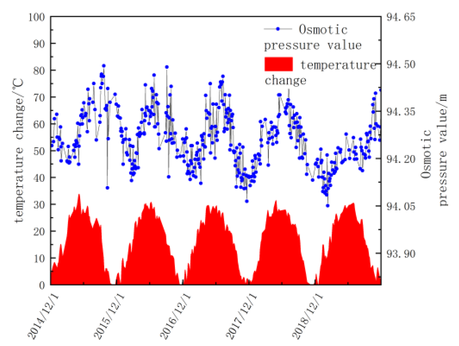
3.1. Water Level and Temperature Safety Evaluation Standard

Water level and temperature are important environmental factors that affect the safety of channel seepage and they are easy to obtain directly through monitoring instruments and are less affected by the outside world. Therefore, water level and temperature are two important indicators in channel monitoring. In seepage safety evaluation, whether the seepage state of the project is evaluated as normal and safe is determined by whether the values of the two monitoring indicators of water level and temperature are reasonable: when the measured value is within the range specified by the monitoring indicators, the project is generally considered to be in a normal condition; otherwise, there is a possibility of destruction.

The determination method of the monitoring index value method is shown in Figure 5 and Equations (6) and (7). First, the data are divided into several regions according to the data’s distribution state. The regions are divided by determining the center and considering the deviation of the observed values on the upper and lower sides of the center. For those observation items whose measured value is too large or too small, such as temperature, the y-value division should be considered bilaterally; for those observation items whose measured value is too small or too large, there is a problem, and for the measured value that is too small but beneficial, such as the osmotic pressure value data, the y-value partition can be considered only as a large one-sided consideration.

$$\begin{array}{l}AreaA:y\le [y_{\max }],andy\le \overline{y}+S;\\ AreaB:y\le [y_{\max }],and\overline{y}+S\le y\le \overline{y}+2S\\ AreaC:y\le [y_{\max }],andy>\overline{y}+2S\\ AreaD:y>[y_{\max }],andy\le \overline{y}+2S\\ AreaE:y>[y_{\max }],andy>\overline{y}+2S\end{array}\}$$

(6)

$$\begin{array}{l}AreaA:[y_{\min }]\le y\le [y_{\max }],and\overline{y}-S\le y\le \overline{y}+S\\ AreaB:[y_{\min }]\le y\le [y_{\max }],and\overline{y}+S\le y\le \overline{y}+2Sor\overline{y}-2S\le y\le \overline{y}-S\\ AreaC:[y_{\min }]\le y\le [y_{\max }],andy>\overline{y}+2Sory<\overline{y}-2S\\ AreaD:y>[y_{\max }]ory<[y_{\min }],andy\le \overline{y}+2Sory\ge \overline{y}-2S\\ AreaE:y>[y_{\max }]ory<[y_{\min }],andy>\overline{y}+2Sory<\overline{y}-2S\end{array}\}$$

(7)

In the formula, S is the remaining standard deviation of the model.

(1)

Water level safety evaluation standard in the canal

For channel water flow, its water level data usually remain stable and its data do not vary greatly but its value changes should have a corresponding warning water level. Therefore, the upper-limit value of the water level is selected as $[y_{max}]$. The measured data were calculated for many years. After obtaining the average value of the water level data $\overline{y}$, the standard deviation value S, the historical maximum water level $\left[y_{max}\right]$, and the minimum water level $y_{min}$, the corresponding evaluation standard set is established as follows (See

Table 1. Establishment of the water level data grading standard.

Grading	Grading Standard
Safety 75~100%	$y\le \left[y_{max}\right],and y_{min}\le y\le \overline{y}+S$
Safety 50~75%	$y\le \left[y_{max}\right],and \overline{y}+S\le y\le \overline{y}+2S$
Safety 25~50%	$y\le \left[y_{max}\right],and \overline{y}+2S\le y\le y_{max}$
Safety 0~25%	$y\le \left[y_{max}\right],and y\ge y_{max}$

Note: y denotes the measured value; $\overline{y}$ denotes the average value of the water level data; $\left[y_{max}\right]$ denotes the water level warning value; and S denotes the standard deviation of the monitoring data.

):

(2)

Temperature Evaluation Safety Standards

The temperature change around the channel usually changes periodically with the change in the seasons. The data have a large range of up and down changes, and temperatures rise and drop due to temperature effects. Therefore, it is necessary to convert the changes in temperature data for many years into data calculations during periods of temperature rise and drop. From this, the average temperature $\overline{y}$ and the standard deviation value $S$ of the two periods can be obtained, and the highest and lowest temperature values can be combined to establish the evaluation standard set (See

Table 2. Temperature class aging standards.

Temperature Drop		Temperature Rise
Grading	Grading Standard	Grading	Grading Standard
Safety 75~100%	$y\ge \left[y_{min}\right],and \overline{y}-S\le y\le y_{max}$	Safety 75~100%	$y\le \left[y_{max}\right],and y_{min}\le y\le \overline{y}+S$
Safety 50~75%	$y\ge \left[y_{min}\right],and \overline{y}-2S\le y\le \overline{y}-S$	Safety 50~75%	$y\le \left[y_{max}\right],and \overline{y}+S\le y\le \overline{y}+2S$
Safety 25~50%	$y\ge \left[y_{min}\right],and \le y<\overline{y}-2S$	Safety 25~50%	$y\le \left[y_{max}\right],and \overline{y}+2S\le y\le y_{max}$
Safety 0~25%	$y\ge \left[y_{min}\right],and y<y_{\min }$	Safety 0~25%	$y\le \left[y_{max}\right],and y\ge y_{max}$

Note: $y$ denotes the measured value; $\overline{y}$ denotes the average value of the data; $\left[y_{max}\right]$, $\left[y_{min}\right]$ denote the upper-limit temperature and the lower-limit temperature, respectively; $S$ denotes the standard deviation of the monitoring data; and $y_{max}$ and $y_{min}$ denote the highest and lowest temperature values, respectively, of the historical data.

):

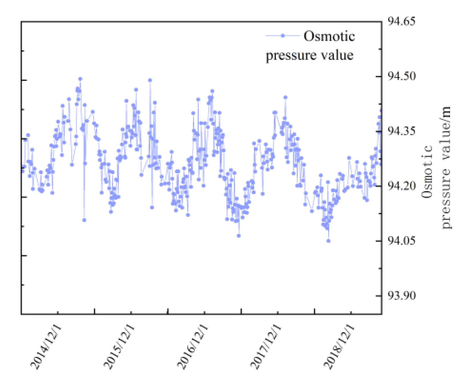
3.2. Osmotic Pressure Safety Evaluation Standard

In the safety evaluation of channel seepage, the change in seepage pressure (also known as the pore water pressure) is the main reference for the stability of the seepage. The piezometer is not only closely related to the channel water level, temperature, and other data but is also easily affected by surrounding soil factors and boundary conditions. Therefore, compared with water level and temperature, osmotic pressure data are strongly uncertain.

When determining the osmotic pressure safety evaluation standard, its strong uncertainty characteristics should be fully considered. Therefore, based on the measured osmotic pressure data, this paper adopts cloud model theory to establish the osmotic pressure safety evaluation standard.

(1)

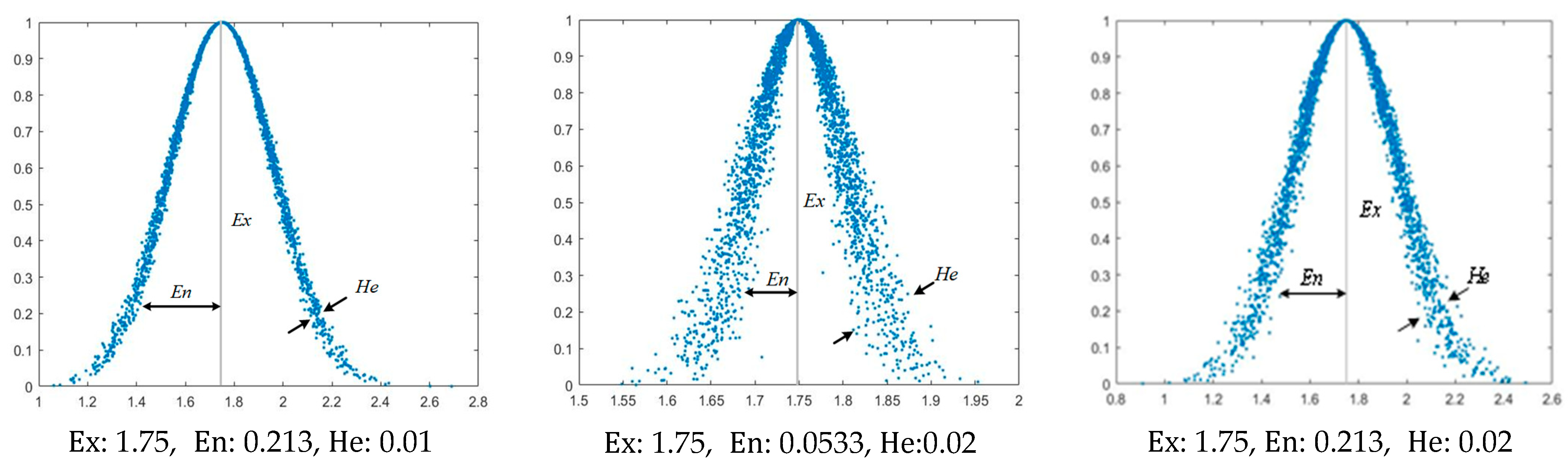
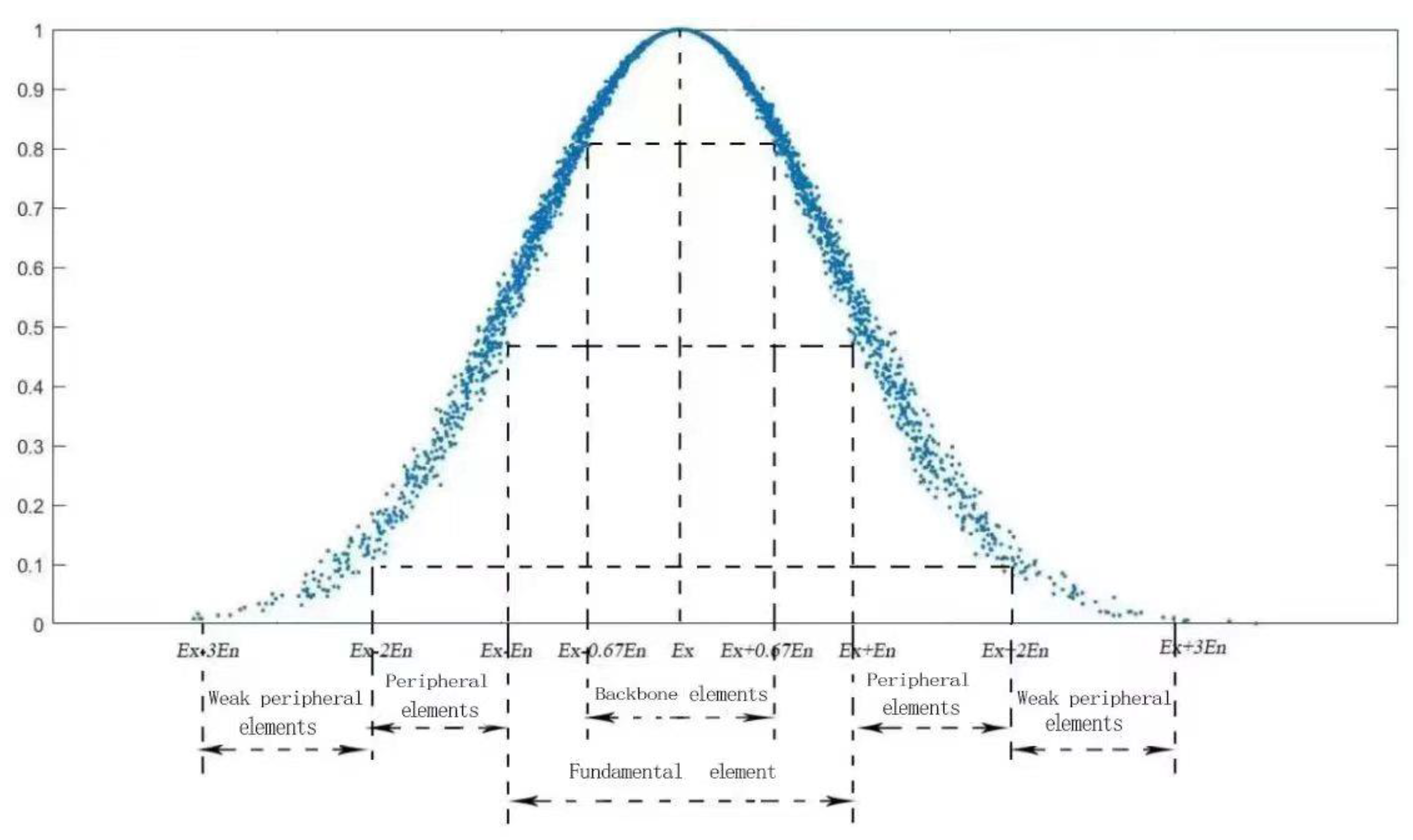
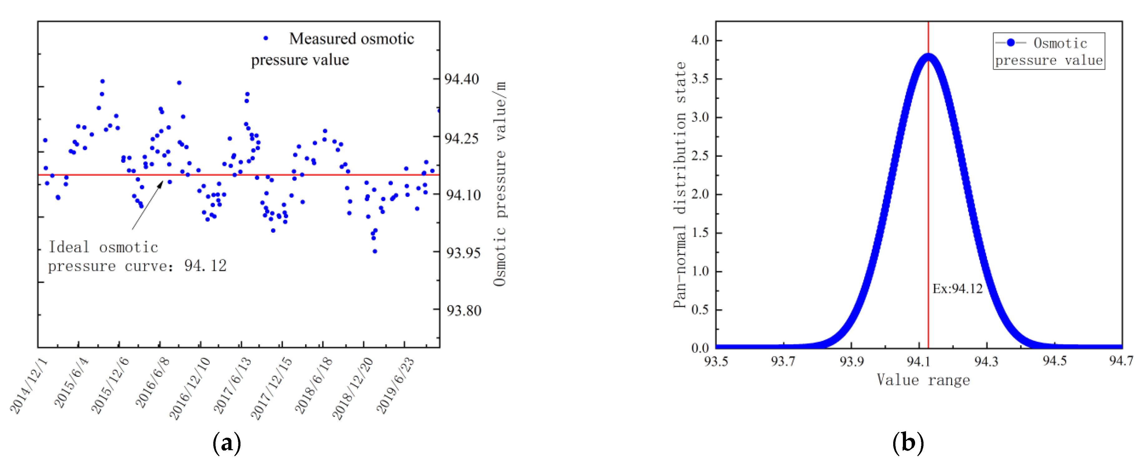
Cloud model theory:

The cloud model is a modern mathematical theory proposed by academician Li Deyi [13] on the basis of traditional fuzzy set theory and probability and statistics theory; cloud model theory specializes in the study of compound uncertainty [22] and can better describe variables. Randomness, ambiguity, and their relevance, to realize the mapping and conversion between qualitative and quantitative uncertainties, have been applied in state diagnosis and comprehensive evaluations in many fields [23,24].

Suppose U is a quantitative domain represented by a numerical value, and suppose C is a qualitative concept on U. If the quantitative numerical value $x\in U$ is a random realization of the qualitative concept C, the certainty of x to C, $\mu \left(x\right)\in [0,1]$, is a random number with a stable tendency, which is

$$\mu :U\to [0,1],\forall x\in U,x\to \mu \left(x\right)$$

(8)

Then, the distribution of x on the universe of U is called the cloud model. This distribution is referred to as a cloud and is denoted as $C(x)$; each x is called a cloud drop.

A cloud generator is a specific algorithm for mutual conversion between qualitative concepts and quantitative data in a cloud model. The forward cloud generator realizes the conversion from a qualitative concept to a quantitative value, and cloud drops are generated from the digital characteristics of the cloud $(Ex,En,He)$, as shown in Figure 6. The reverse cloud generator realizes the conversion from a quantitative value to a qualitative concept. The generator converts accurate data into a qualitative concept represented by cloud digital features $(Ex,En,He)$, as shown in Figure 7. The specific algorithm is as follows:

• Calculate the sample mean $\overline{x}=\frac{1}{n}{\displaystyle \sum _{i=1}^n{x}_i}$ of the basic data according to $x_i$, the absolute center distance of the first-order sample $\frac{1}{n}{\displaystyle \sum _{i=1}^n}|x_i-\overline{x}|$, and the sample variance $S^2=\frac{1}{n-1}{\displaystyle \sum _{i=1}^n}{(x_i-\overline{x})}^2$
• $Ex=\overline{x}$
• $En=\sqrt{\frac{\pi }{2}}\times \frac{1}{n}{\displaystyle \sum _{i=1}^n\left|x_i-Ex\right|}$
• $He=\sqrt{\left|S^2-E{n}^2\right|}$

The existence of hyper-entropy $He$ makes the cloud model distribution exist in two states. When the value of is small, cloud drop b assumes a pan-normal distribution. In extreme cases, that is, when the value of $He$ is 0, the discrete cloud drops outline the shape of a normal distribution. With the continuous increase in $He$, the distribution of cloud drops enters a state of obvious fogging: the expected curve of the cloud is no longer obvious, the outer cloud drops are more scattered, and the core cloud drops have a clear centralization trend (Figure 8). According to relevant studies [25,26,27], the state of the cloud model is demarcated at $He=\frac{En}{3}$; that is, when $He<\frac{En}{3}$, the cloud drop shows a pan-normal state; otherwise, the cloud drops are in an atomized state.

Therefore, according to the distribution of cloud drops, the cloud model theory proposes the “3$En$ rule” for cloud drops under a normal distribution (Figure 9); that is, for the universe of U, the quantitative value that contributes to the qualitative concept falls mainly within the range of $[Ex-3En,Ex+3En]$, and the contribution of the data in this interval to the qualitative concept accounts for approximately 99.74% of the total data. The elements in the interval $[Ex-En,Ex+En]$, the intervals $[Ex-2En,Ex-En]$ and $[Ex+En,Ex+2En]$, and the intervals $[Ex-3En,Ex-2En]$ and $[Ex+2En,Ex+3En]$ each account for 33.33% of the total elements, but these elements are qualitative. The contribution of the concept is 68.26%, 27.18%, and 4.3%, respectively. When the cloud drop distribution is in an atomized state, the cloud drop distribution is also characterized by central clustering or local cloud droplets gathering into clusters, but it is impossible to determine the contribution of specific data to the qualitative concept.

According to the above analysis, when cloud model theory transforms quantitative data into qualitative concepts, its core idea is to use qualitative-concept cloud digital features to show the uncertainty contained in quantitative data, but the change in hyper-entropy is the main factor that affects the distribution of cloud models. Generally, the greater the hyper-entropy is, the greater the uncertainty of the data, the more disorderly the distribution of the data, and the more difficult it is to ensure the regularity of data changes. Additionally, the interval determined by expectation and entropy determines the contribution of each part of the data to the qualitative concept. Therefore, the cloud digital feature that represents the qualitative concept is regarded as a specific value, combined with the establishment method of the previous environmental factor evaluation standard set, and the evaluation standard set of the osmotic pressure value is established.

(2)

Determination of the osmotic pressure safety evaluation standard

The monitoring data of osmotic pressure are shown in Figure 10. Figure 10a shows that the actual osmotic pressure value curve is floating around the ideal osmotic pressure value curve. After the data are processed, as shown in Figure 10a, the statistical law can be obtained, as shown in Figure 10b.

Considering cloud model theory [28,29,30], we can see that there are two meanings in the expectation of $Ex$ in cloud digital features. One is the qualitative concept. It is expected that $Ex$ represents the most frequently occurring data of the qualitative concepts and is the most representative of the qualitative concepts in the model. The value is the mathematical expectation of the cloud drop in the spatial distribution of the universe. The second is the numerical concept, which represents the mean value of the quantitative data; because the actual osmotic pressure value curve fluctuates around the ideal osmotic pressure value curve, by using the reverse cloud generator and by converting the basic data of the osmotic pressure value into $Ex$, we can determine the value of the osmotic pressure data that best represents the qualitative concept of the osmotic pressure value under the influence of many uncertain conditions.

Entropy $En$ represents the uncertainty measurement of a qualitative concept and is determined by the randomness and ambiguity of the concept. On the one hand, $En$ is a measure of the randomness of the qualitative concept and thus represents the degree of dispersion of the cloud drops in this qualitative concept. The random range of the appearance of the cloud drops, which represents the qualitative concept, represents the probability of the actual osmotic pressure value appearing under external conditions. On the other hand, this range also reflects the value range of the cloud drops that can be conceptually accepted in the universe of discourse; that is, this range determines the value range of the osmotic pressure value under the existing data.

Hyper-entropy $He$ represents the uncertainty of entropy, thereby reflecting the cohesion of random variables corresponding to the qualitative concept, that is, the randomness of random variables; $He$ represents the probability of the data reappearing at each point in the cloud model graph. The smaller $He$ is, the greater the possibility that the data value will appear again. The performance of the osmotic pressure data is reflected in the regularity of the data. The stronger the regularity of the data is, the smaller the $He$ of the data.

Combined with the above analysis, the standard values of the osmotic safety evaluation gradings set here are as follows (combined with Figure 9 and Figure 10b): The cloud model theory requires performing reverse cloud computing of the measured data and transforming the cloud digital characteristics’ qualitative concepts into numerical data. The distribution characteristics are evaluated by the formula $He=\frac{En}{3}$. For the osmotic pressure data under the pan-normal distribution, the “3$En$ rule” should be considered in combination to realize the evaluation standard set setting. When the data are in a pan-normal distribution, because the data distributed in the interval $[Ex,Ex+En]$ are closest to the expectation $Ex$ in terms of numerical performance, the data are set to have the highest degree of safety in this interval; specifically, the safety degree is 75~100%, and the data in the intervals $[Ex+En,Ex+2En]$ and $[Ex+2En,Ex+3En]$ decrease successively because of the data’s contribution to the determination of the qualitative concept. In terms of numerical performance, the distance from the expected $Ex$ value increases successively, so the safety degree is set to decrease successively, and the safety degree is 50~75% and 25~50%, successively; for data exceeding the interval $[Ex+3En,y_{\max }]$, the safety degree is at least 0~25%.

When the cloud drop distribution is in an atomized state, that is, at time $He>\frac{En}{3}$, because the data are clustered or converged in a central area in the interval $[Ex,Ex+3En]$ at this time, although the measured data have a poor expression of the qualitative concept, overall its distribution of the data is in a messy state, so the standard set of the dynamic gradings of osmotic pressure can be established through the mean and standard deviation of the data, as shown in

Table 3. Aging standards for the dynamic grading of osmotic pressure values.

$\mathit{H}\mathit{e} < \frac{\mathit{E}\mathit{n}}{3}$		$\mathit{H}\mathit{e} \ge \frac{\mathit{E}\mathit{n}}{3}$
Grading	Grading Standard	Grading	Grading Standard
Safety 75~100%	$\left[y_{min},Ex+En\right]$	Safety 75~100%	$\left[y_{min},\overline{y}+S\right]$
Safety 50~75%	$\left[Ex+En,Ex+2En\right]$	Safety 50~75%	$\left[\overline{y}+S,\overline{y}+2S\right]$
Safety 25~50%	$\left[Ex+2En,Ex+3En\right]$	Safety 25~50%	$\left[\overline{y}+2S,\overline{y}+3S\right]$
Safety 0~25%	$\left[Ex+3En,y_{max}\right]$	Safety 0~25%	$\left[\overline{y}+3S,y_{max}\right]$

Note: $y_{max},y_{min}$ denote the maximum and minimum values of osmotic pressure, respectively.

.

4. Analysis of the Seepage Safety Evaluation of the Canal in a High-Fill Section

In this section, the high-fill canal section SH(3)124+525 is taken as an example and the above method is used to evaluate the canal’s seepage safety.

4.1. Establishment of Evaluation Index System and Evaluation Standard Set

The high-fill canal section is based on the piezometer monitoring points close to the canal; these points are indicated as P4-4 and P4-6. Therefore, for canal section SH(3)124+525, piezometer P4-6 was selected for analysis. For the rest of the canal data, piezometers P5-4, P6-5, and P7-5 were used.

The evaluation index system is as

Table 4. Evaluation index values of engineering safety osmotic monitoring data.

Evaluation Index	Water Level Data	Temperature Change	Osmometer P4-6	Osmometer P5-4	Osmometer P6-5	Osmometer P7-5
Osmotic index value	108.45	14.9	93.99	93.95	93.52	92.68

, in which the temperature selects the data under the temperature rise state:

According to Section 4.1 and Section 4.2, the following data can be obtained by calculating water level data, temperature data during temperature rise and temperature drop, and osmotic pressure data.

According to historical data, the minimum water level data was 87.13 m, the maximum value was 112.17 m, the average value was 106.92 m, the water level standard deviation S was 2.26, and the water level upper-limit value was 115.15. Therefore, the following evaluation criteria set can be obtained (See

Table 5. Evaluation standard set of water level data in the channel.

Grading	Grading Standard
Safety 75~100%	[87.13, 109.18]
Safety 50~75%	(109.18, 111.43]
Safety 25~50%	(111.43, 112.17]
Safety 0~25%	(112.17, 115.15]

):

According to the actual project, the temperature rise phase was set here from March to November, and the temperature drop phase was from December to February of the next year. The following data were obtained: During the temperature rise period, the lowest temperature was 2.30 °C, the highest temperature was 38.70 °C, the average value was 21.11 °C, the temperature standard deviation was 7.9 °C, and the set upper-limit temperature was 41.50 °C. During the temperature drop stage, the highest temperature was 12.30 °C, the lowest temperature was −10.40 °C, the average value was 2.93 °C, the temperature standard deviation was 4.42 °C, and the set lower-limit temperature was −15.60 °C. The specific evaluation standard set is as

Table 6. Temperature evaluation standard set.

Temperature Drop		Temperature Rise
Grading	Grading Standard	Grading	Grading Standard
Safety 75~100%	[−1.49, 12.30]	Safety 75~100%	[2.30, 29.01]
Safety 50~75%	(−5.91, −1.49]	Safety 50~75%	(29.01, 36.91]
Safety 25~50%	(−10.40, −5.91]	Safety 25~50%	(36.91, 38.70]
Safety 0~25%	[−15.60, −10.40]	Safety 0~25%	(38.70, 41.50]

:

According to the channel osmotic pressure layout, the calculation results of the average value, entropy value, and super entropy of the channel osmometer are shown in the following table, and the corresponding grading standards are shown in

Table 7. Calculation results of the osmometer data.

Osmometer Number	Mean (Ex)	Entropy (En)	Hyper-Entropy (He)	Max	Min
Osmometer P4-6	94.12	0.19	0.06	95.52	93.59
Osmometer P5-4	93.47	0.18	0.03	94.09	92.90
Osmometer P6-5	93.37	0.12	0.01	93.85	92.87
Osmometer P7-5	92.63	0.16	0.05	93.32	92.14

:

According to the calculation result, $He<\frac{En}{3}$ can be obtained. The evaluation standard set of the osmotic pressure values is as

Table 8. Evaluation standard set of osmotic pressure values.

Osmometer P4-6		Osmometer P5-4
Grading	Grading standard	Grading	Grading standard
Safety 75~100%	[93.59, 94.31)	Safety 75~100%	[92.90, 93.65)
Safety 50~75%	[94.31, 94.50)	Safety 50~75%	[93.65, 93.83)
Safety 25~50%	[94.50, 94.70)	Safety 25~50%	[93.83, 94.01)
Safety 0~25%	[94.70, 95.52]	Safety 0~25%	[94.01, 94.09]
Osmometer P6-5		Osmometer P7-5
Grading	Grading standard	Grading	Grading standard
Safety 75~100%	[92.87, 93.49)	Safety 75~100%	[92.14, 92.79)
Safety 50~75%	[93.49, 93.61)	Safety 50~75%	[92.79, 92.95)
Safety 25~50%	[93.61,93.73)	Safety 25~50%	[92.95,93.11)
Safety 0~25%	[93.73,93.85]	Safety 0~25%	[93.11,93.32]

:

4.2. Weight Distribution

Using the analytic hierarchy process, the weights were determined as

Table 9. Index weights of channel osmotic safety evaluation.

Evaluation Index	Water Level Data	Temperature Change	Osmometer P4-6	Osmometer P5-4	Osmometer P6-5	Osmometer P7-5
Weights	0.0812	0.0673	0.2235	0.2171	0.2122	0.1987

:

4.3. Connection Calculation

(1)

Single index connection degree

According to the connection number expressions (2)–(5) in Section 2.2.3, the connection degree between the six evaluation indices of channel osmotic safety and the four evaluation grading standard limits can be obtained. The details are as follows:

Water level data:     $\begin{array}{l}{\mu }_1=1+0i+0j\\ {\mu }_2=0.7550+0.2450i+0j\\ {\mu }_3=0.1989+0.6048i+0.1962j\\ {\mu }_4=0.4448+0.1104i+0.448j\end{array}$	Osmometer P5-4:     $\begin{array}{l}{\mu }_1=0.9968+0.0019i+0.0018j\\ {\mu }_2=0.6051+0.3949i+0j\\ {\mu }_3=1+0i+0j\\ {\mu }_4=0.5341+0.4659i+0j\end{array}$
Temperature change:     $\begin{array}{l}{\mu }_1=1+0i+0j\\ {\mu }_2=0.3589+0.6411i+0j\\ {\mu }_3=0.0752+0.3319i+0.5929j\\ {\mu }_4=0.1053+0.0673i+0.8274j\end{array}$	Osmometer P6-5:     $\begin{array}{l}{\mu }_1=0.9997+0.0003i+0j\\ {\mu }_2=1+0i+0j\\ {\mu }_3=0.5852+0.4148i+0j\\ {\mu }_4=0.3751+0.3657i+0.2592j\end{array}$
Osmometer P4-6:     $\begin{array}{l}{\mu }_1=1+0i+0j\\ {\mu }_2=0.3734+0.6266i+0j\\ {\mu }_3=0.2719+0.2719i+0.4563j\\ {\mu }_4=0.5359+0.1252i+0.3353j\end{array}$	Osmometer P7-5:     $\begin{array}{l}{\mu }_1=1+0i+0j\\ {\mu }_2=0.5901+0.4099i+0j\\ {\mu }_3=0.3711+0.3711i+0.2578j\\ {\mu }_4=0.3219+0.2516i+0.4265j\end{array}$

(2)

Comprehensive connection degree

According to the formula $W\cdot \mu$, the comprehensive connection degree vector H is carried out:

$$W=[0.0812,0.0673,0.2122,0.2171,0.2235,0.1987]$$

$$H=W\cdot \mu =\left[\begin{array}{l}0.9992+0.0005i+0.0003j\\ 0.6368+0.3632i+0j\\ 0.5005+0.2956i+0.2039j\\ 0.4214+0.2729i+0.3056j\end{array}\right]$$

4.4. Evaluation Results

From the calculation result H of the above comprehensive connection degree matrix, combined with the definition of the generalized set pair potential, four levels of generalized set pair potential values were calculated, and normalized processing was performed to calculate the confidence interval. The calculation results are shown in

Table 10. Set pair theory evaluation results.

Grading Index	Safety 75~100%	Safety 50~75%	Safety 25~50%	Safety 0~25%
Osmotic $SHI{\left({\mu }_1\right)}_G$	2.7155	1.8904	1.3453	1.1228
$f_i$	0.3839	0.2672	0.1902	0.1587
Confidence interval		0.6511

.

According to the normalized generalized set pair potential value in the table, the confidence criterion was used to judge, and the security level of the channel was obtained as “safety degree 50~75%”.

4.5. Test Information Verification

In terms of inspection information verification, nondestructive inspection methods, namely, geological radar, high-density electrical methods, and surface wave methods, were used mainly to realize the internal abnormality judgment of the channel. The ground-penetrating radar method was aimed mainly at detecting the soil within 10 m of the channel section, while the high-density electrical method and the surface wave method were aimed mainly at detecting the depth of 5–30 m. Therefore, combining the above three methods can realize the characteristic analysis of the spatial distribution of the soil information caused by channel seepage by using tomography to determine whether, based on the figure information and data, there are potential safety hazards in the channel section and combining tomography with the analysis results of the monitoring dataset to realize mutual verification.

The working configuration was determined according to the site conditions. The geological radar was generally arranged on the road surface on both sides of the channel, facing the downstream direction, from the left bank to the right bank. The high-density electrical method was furnished at the unhardened position of the embankment toe or the top of the embankment on the outside of the road surface, and the survey line numbers were GZ1 and GY1 in turn; the surface wave method was the same as the high-density electrical method. The line numbers were MZ1 and MY1 in sequence. The layout diagram can be seen Figure 11 and Figure 12.

The ground-penetrating radar adopted the SIR-3000 ground-penetrating radar produced by GSSI Company in the United States and adopted a 100 Mz shielded antenna. The high-density electrical method employed the WDJD-3 multifunctional digital DC IP instrument of Chongqing Pentium, as shown in the Figure 13, with multiple high-density cables and special copper electrodes; the surface wave exploration used the Geode-24 engineering seismograph produced in the United States, as shown in the Figure 14. A 26-pound sledgehammer was used as the source, a 4.0 Hz vertical detector was used to receive the signal, and the 2 m and 5 m track spacing detector cables were in employment.

(1)

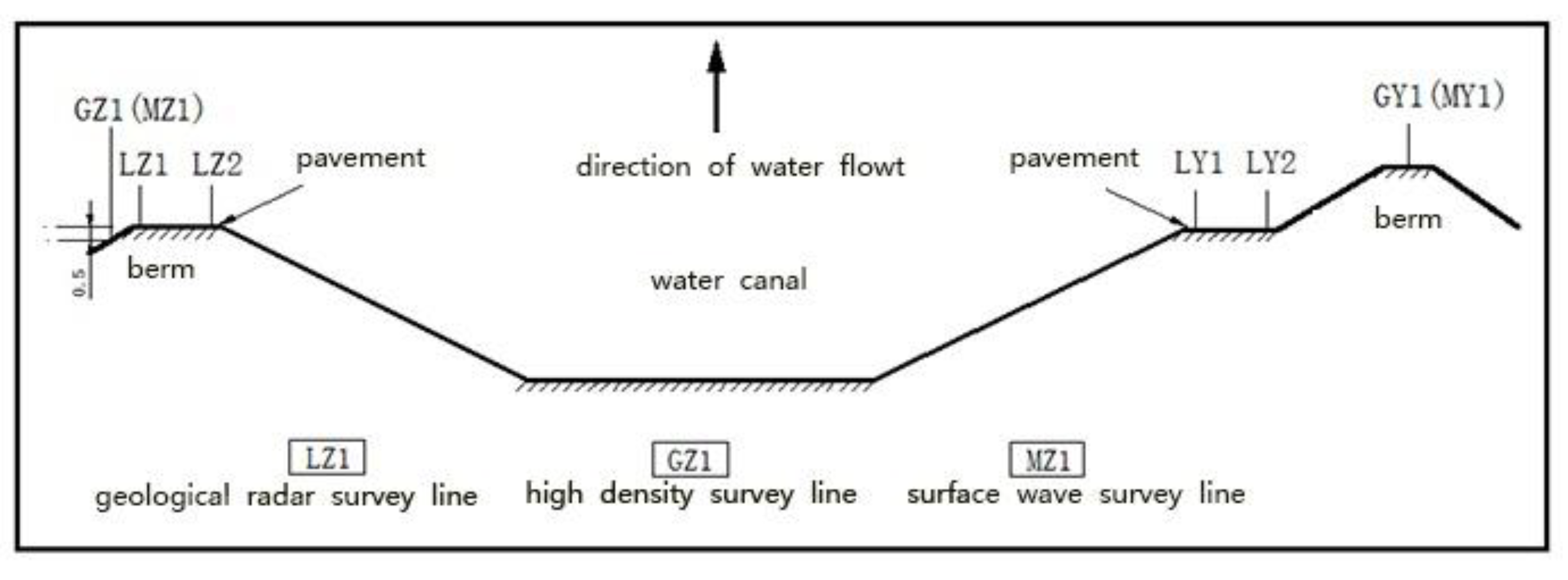
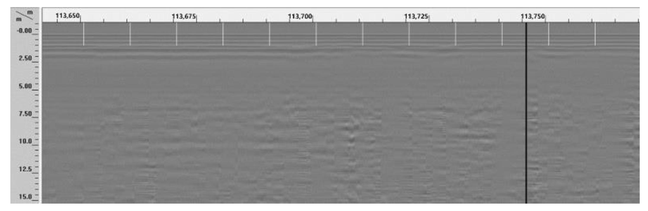
Geological radar method

Four survey lines were arranged. The radar profile near the underpass of each survey line is shown in Figure 15, Figure 16, Figure 17 and Figure 18 and the black line in the figure indicates the position of the underpass; the left bank survey line numbers were LZ1 and LZ2 (See Figure 15 and Figure 16) and the right bank survey line numbers were LY1 and LY2. The test ranges of the four survey lines were as follows:

The test range of the LZ1 line was from the stake number SH(3)124+525 to H(3)124+953.5; the test range of the LZ2 line was SH(3)124+524~SH(3)124+953.5; the test range of the LY1 line was from the stake number SH(3)125+053.5 to SH(3)125+453.5; and the test range of the LY2 line was SH(3)125+053.5~SH(3)125+452.5. Analyzing the radar profile revealed no anomalies, such as the misalignment of the event axis, cluttered reflected waves, or double arcs of strong reflections, thereby showing that there were no obvious defects, such as voids or subsidence, in the underground soil within the detection range of the geological radar.

(2)

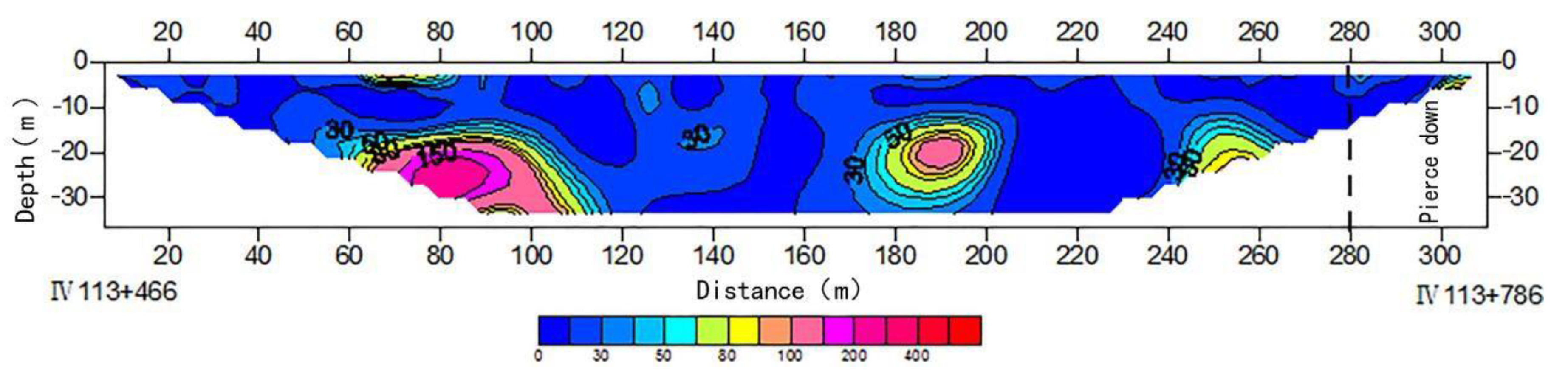
High-density electrical method

The high-density electrical method completed two survey lines: the left bank survey line number was GZ1 and the resistivity profile is shown in Figure 19; the right bank survey line number was GY1 and the resistivity profile is shown in Figure 20.

Survey line GZ1: the resistivity profile (Figure 19) shows that the overall resistivity was low and uniform, and the resistivity was basically below 40 Ω·m, thus indicating that the underground soil quality was relatively uniform and that there were no obvious defects in the detection range. Survey line GY1: the resistivity profile (Figure 20) shows that most of the resistivity was below 40 Ω·m. When the horizontal distance was 60~110 m, the depth was 15~33 m; when the horizontal distance was 180~200 m, the depth was 12~28 m; and when the horizontal distance was 245~260 m, the depth was less than 20 m. The area had a relatively high resistance and the resistivity exceeded 50 Ω·m, thereby indicating that the existence of high underground resistance was abnormal. The horizontal distance was 180~200 m and the depth was 12~28 m. The area was a closed high-resistance area and may have been a gravel area. It was recommended to check regularly later; according to the overall profile, the high resistance of the other two parts should have been caused by changes in the soil quality, and the possibility of defects was small. In general, the two measuring lines had no obvious abnormalities near the underpass project, and the possibility of defects was small.

(3)

Surface wave method

The MZ1 survey line was located on the grassland on the outer slope of the left bank road. Thirty points were tested, and the test results are shown in Figure 21. The black dashed line in the figure indicates the possible position of the underpass project. The figure shows that although the wave speed was chaotic, from top to bottom, the wave speed gradually increased at depths of 5 m, 10 m, 17 m, 27 m, and below, thus indicating that the underground medium was relatively uniform in the detection range and that there was no obvious defect.

The MY1 survey line was located on the grassland on the top of the slope on the outside of the right bank road. The test result is shown in Figure 22. The black dashed line in the figure indicates the possible position of the underpass project. The figure shows that the wave speed of the underground medium gradually increased with increasing depth, thus indicating that the soil was dense and had no obvious defects within the detection range.

4.6. Results of Fusion Analysis of Monitoring Data and Detection Information

The quantitative evaluation of the monitoring data was accomplished according to the set pair analysis method. Combining with the actual channel engineering, a method based on the set-pair analysis method and a fusion of the various theoretical methods was explored to realize the quantitative evaluation of the monitoring data. According to the change law and distribution state of the data with the monitoring index value method and the theoretical method of the cloud model, a single-point multi-factor model of the environmental variable and osmotic pressure value was established, respectively. The calculation of the potential and confidence interval and other contents realized the evaluation results of the monitoring data, determined the safety level of the seepage monitoring data under the project, and verified the applicability of the set pair analysis to the project.

Using non-destructive testing methods such as a high-density electrical method, geological radar, and surface wave method, a variety of detection and diagnosis methods in the interior space of the canal section were established and the fusion analysis of monitoring data and detection information was realized. By combining the evaluation results of the monitoring data with the qualitative results of the testing information, the mutual verification between the two was achieved.

In the application example, according to the analysis results of the monitoring dataset, the results of the channel osmotic safety evaluation were all “safety degree 50~75%”. The inspection information showed that there were no obvious defects, such as voids or collapses, in the channel. Therefore, the method provided in this article can realize the safety degree analysis of engineering safety, and after combining with the inspection information, the results can be mutually confirmed, thus indicating the safety of the channel section. The combination of the two is more beneficial to comprehensively evaluate degree of the engineering safety, and this method also provides a new research idea for the safety evaluation of the channel.

5. Conclusions

The seepage pressure date of a water diversion project with a high fill (SH(3)124+525, SH(3)124+953.5, SH(3)125+053.5, SH(3)125+453.5) was taken as an example to establish a seepage flow safety evaluation model combining with detection information to realize the safety evaluation of channel seepage. The specific conclusions are as follows:

(1)

Combining the monitoring index value method and the theoretical method of the cloud model, a single-point multi-factor aging model of the monitoring data can be established. Through statistical analysis of the monitoring data, the data mean Y, standard deviation value S, and cloud digital characteristics can be obtained. On the premise of clarifying the distribution interval of monitoring data, safety evaluation standards for factors such as water level, temperature, and osmotic pressure are obtained.

(2)

Integrating the single-point multi-factor aging model with the set pair analysis method can realize the determination of the evaluation level of monitoring data. Using the formula of the connection degree, the generalized set pair potential, and confidence intervals, etc., the safety level of the seepage monitoring data of the project is determined, and the safety evaluation result is “safety degree 50~75%”.

(3)

The detection of abnormal information could be realized. By collecting data a from a geological radar and using the high-density electrical and surface wave method to achieve an image output using tomography and other methods, the qualitative analysis of canal section safety is realized based on expert experience.

(4)

With the employment of the comprehensive analysis method, the relationship between environmental variables, monitoring data, and detection information is studied and considered, an adaptive evaluation method reflecting the working behavior of the channel is established, and corresponding diagnostic techniques are proposed.

References

- Ge, W.; Li, Z.K.; Liang, R.Y.; Li, W.; Cai, Y.C. Methodology for Establishing Risk Criteria for Dams in Developing Countries, Case Study of China. Water Resour. Manag. 2017, 31, 4063–4074. [Google Scholar] [CrossRef]
- Matalas, N.C.; Nordin, C.F.; Ministry of Water Resources of the People’s Republic of China. First National Water Conservancy Survey Bulletin; China Water Resources and Hydropower Press: Beijing, China, 2013. [Google Scholar]
- Fan, Q.; Tian, Z.; Wang, W. Study on Risk Assessment and Early Warning of Flood-Affected Areas when a Dam Break Occurs in a Mountain River. Water 2018, 10, 1369. [Google Scholar] [CrossRef] [Green Version]
- Jie, J.; Sun, D. Statistics of Dam Damages in China and Analysis on Damage Causations. Water Resour. Hydropower Eng. 2009, 40, 124–128. [Google Scholar]
- Jiang, S.; Fan, Z. Earth-rockfill dam safety classification and risk rate assessment on flood control. J. Hydraul. Eng. 2008, 39, 35–40. [Google Scholar]
- Chen, S. The Damage Mechanism of Earth-Rock DAMS and the Simulation of Dam Damage Process; China Water &Power Press: Beijing, China, 2012. [Google Scholar]
- Mei, Y.; Zhong, Y. Fuzzy Extension Evaluation Model of Dam Osmotic Behavior Based on Entropy Weight. Water Resour. Power 2011, 29, 58–61. [Google Scholar]
- Wang, X.; Dai, L.; Lü, P.; Wang, C.; Cheng, Z. Study on Comprehensive Evaluation Model of Osmotic Safety Based on DSR-Extension Cloud. J. Tianjin Univ. 2019, 52, 52–61. [Google Scholar]
- Wang, X.; Yu, H.; Lv, P.; Wang, C.; Zhang, J.; Yu, J. Seepage Safety Assessment of Concrete Gravity Dam Based on Matter-Element Extension Model and FDA. Energies 2019, 12, 502. [Google Scholar] [CrossRef] [Green Version]
- Su, H.; Ou, B.; Fang, Z.; Gao, J.; Wen, Z. Dual criterion-based dynamic evaluation approach for dike safety. Struct. Health Monit. 2018, 18, 147592171881337. [Google Scholar] [CrossRef]
- Xiang, Y.; Fu, S.; Zhu, K.; Yuan, H.; Fang, Z. Seepage safety monitoring model for an earth rock dam under influence of high-impact typhoons based on particle swarm optimization algorithm. Water Sci. Eng. 2017, 10, 70–77. [Google Scholar] [CrossRef]
- Lan, Z.; Huang, M. Safety assessment for seawall based on constrained maximum entropy projection pursuit model. Nat. Hazards 2018, 91, 1165–1178. [Google Scholar] [CrossRef]
- Su, H.; Tian, S.; Kang, Y.; Xie, W.; Chen, J. Monitoring water seepage velocity in dikes using distributed optical fiber temperature sensors. Autom. Constr. 2017, 76, 71–84. [Google Scholar] [CrossRef]
- Keqin, Z. Set pair analysis and its prelimiary application SE. Explor. Nat. 1994, 13, 67–72. [Google Scholar]
- Cao, L.; Wang, H.Y.; Lu, F.X. Operational Capability Evaluation of Surface Warship Formation Based on Set Pair Analysis. In Proceedings of the 2016 8th International Conference on Intelligent Human-Machine Systems and Cybernetics (IHMSC), IEEE, Hangzhou, China, 27–28 August 2016. [Google Scholar]
- Yang, Y. Research on approximate inference method based on Set pair logic. CAAI Trans. Intell. Syst. 2015, 10, 921–926. [Google Scholar]
- Li, W. Application of AHP Analysis in Risk Management of Engineering Projects. J. Beijing Univ. Chem. Technol. 2009, 1, 46–48. [Google Scholar]
- Cui, D.H.; Zhang, X.Y. Application of Gray Analytic Hierarchy Process in Project Risk Evaluation. In Proceedings of the 2009 International Conference on Artificial Intelligence and Computational Intelligence, AICI ‘09, Shanghai, China, 7–8 November 2009. [Google Scholar]
- Liu, B.X.; Zhang, C.Y. The Situation Ordered Structure of IDO Connection Degree and ITS Application. In Proceedings of the IEEE 2006 International Conference on Machine Learning and Cybernetics, Dalian, China, 13–16 August 2006. [Google Scholar]
- Li, D.S.; Xu, K.L. IDO most superior pattern recognition model and its application in the safety assessment of the coal mine. Procedia Eng. 2011, 26, 2059–2064. [Google Scholar]
- Yang, Y.F.; Yang, A.M.; Zhang, H.C. Application of Set pair analysis in the Material Clustering. Appl. Mech. Mater. 2013, 443, 707–710. [Google Scholar] [CrossRef]
- Chen, S.; Wang, S.Y.; Sun, J.Z. Trusted software reliability measures based on cloud model. Appl. Res. Comput. 2014, 31, 2729–2731. [Google Scholar]
- Zhou, J.; Zhu, Y.Q.; Chai, X.D.; Tang, W.Q. Approach for analyzing consensus based on cloud model and evidence theory. Syst. Eng. Theory Pract. 2012, 32, 2756–2763. [Google Scholar]
- Zhang, Q.-W.; Zhang, Y.-Z.; Zhong, M. A cloud model base approach for multi-hierarchy fuzzy comprehensive evaluation of reservoir-induced seismic risk. J. Hydraul. Eng. 2014, 45, 87–95. [Google Scholar]
- Chen, H.; Bing, L.I. Gauss Cloud Model Based on Uniform Distribution. Comput. Sci. 2016, 43, 238-241, 246. [Google Scholar]
- Yu, L.; Li, D. Statistics on atomized feature of normal cloud model. J. Beijing Univ. Aeronaut. Astronaut. 2010, 36, 1320. [Google Scholar]
- Li, S.H.; Wang, S.Y.; Zhu, J.D.; Li, B.; Yang, J.; Wu, L.Z. Prediction of rock burst tendency based on weighted fusion and improved cloud model. Yantu Gong Cheng Xue Bao/Chin. J. Geotech. Eng. 2018, 40, 1075–1083. [Google Scholar]
- Gao, H.B.; Zhang, X.Y.; Zhang, T.L.; Liu, Y.C.; Li, D.Y. Research of Intelligent Vehicle Variable Granularity Evaluation Based on Cloud Model. Acta Electron. Sin. 2016, 44, 365–373. [Google Scholar]
- Fu, B.; Li, D.G.; Wang, M.K. Review and prospect on research of cloud model. Appl. Res. Comput. 2011, 2, 420–426. [Google Scholar]
- Wang, S.; Chi, H.; Feng, X.; Yin, J. Human Facial Expression Mining Based on Cloud Model. In Proceedings of the IEEE International Conference on Granular Computing, Nanchang, China, 17–19 August 2009. [Google Scholar]