Article

Economic Growth, CO2 Emissions Quota and Optimal Allocation under Uncertainty

Department of Finance, College of Management, National Yunlin University of Science & Technology, Yunlin 64002, Taiwan
Sustainability 2022, 14(14), 8706; https://doi.org/10.3390/su14148706
Submission received: 16 June 2022 / Revised: 1 July 2022 / Accepted: 4 July 2022 / Published: 16 July 2022

Abstract

:
This study attempts to link greenhouse gas emissions and economic development, and under the premise of considering economic development, proposes an optimal quota of greenhouse gas emissions. Based on the environmental Kuznets curve hypothesis, the logarithmic value of greenhouse gas emissions is an inverted U-shaped function of the logarithmic value of GDP per capita. The empirical results showed that most countries in the world support the Kuznets curve hypothesis. Moreover, using data collected from Our World in Data, the optimal allocation of a greenhouse gas emissions quota can be found by minimizing the uncertainty risk subject to a prespecified global economic growth rate. For government policymakers, they may apply the framework in this study to determine an optimal allocation of greenhouse gas emissions for each sector that will ensure the intended level of domestic economic growth.

1. Introduction

Following the Industrial Revolution in the 18th century, for more than 260 years, human beings have invented tools and innovative technologies in order to both improve their lives and improve their economic standards. Therefore, original resources (such as fossil energy, minerals, and virgin forests) have almost been exhausted, and the destruction of the environment (the shrinking of the ice caps in the Arctic and Antarctic, the deforestation of rainforests leading to biological extinction, etc.) has changed the ecological system, making the Earth no longer able to accept such man-made destruction, and it has begun to remind mankind in its own way (Guggenheim and Al Gore, 2006 [1]; TVBS Sisy’s World News Group, 2010 [2]).

1.1. Climate Change Impacts

On 25 August 2005, a categorized level 5 hurricane, Katrina, caused severe damage in New Orleans, Louisiana, United States. The hurricane made landfall in Florida as a category 1 hurricane, and at dawn on 29 August, it made landfall again on the outer coast of New Orleans, Louisiana, on the Gulf Coast of the United States as a category 3 hurricane. It weakened to a tropical storm more than 12 h after making landfall. According to the United States National Catastrophe Center, Hurricane Katrina was the hurricane/tropical depression that caused the worst damage in the continental United States (Table 1).
In the summer of 2021, the Northern Hemisphere of the Earth was facing a flood. In Western Europe, heavy rains caused flooding in Germany, Belgium, the Netherlands, Luxembourg, and Switzerland. Not only was transportation blocked, but businesses were unable to operate normally, and more complications caused heavy casualties. According to EU statistics, this flood not only extended to five Western European countries, resulting in 228 deaths and 166 missing, but the economic damage was at least 3 billion US dollars.
Moreover, in Asia, from mid-May to mid-July 2018, southwestern China suffered frequent floods in Sichuan, Gansu, and Shaanxi provinces due to the fact of heavy rains for many days, resulting in 3.526 million people being affected, with 16 dead, 4 missing, and a direct economic loss of 1.58 billion Chinese yuan. Two years later, from late May 2020, severe floods were caused by continuous heavy precipitation that occurred in the middle and lower reaches of the Yangtze River, the Huaihe River Basin, Southwest China, South China, and the southeast coast of China. According to China’s official statistics, 63.46 million people were affected by the flood, with more than 54,000 houses collapsed, 247 people dead, and 33 people missing, and the economic damage was over 225.56 billion Chinese yuan.
Deadly floods in Asia, the Arctic melting, droughts in Taiwan, and wildfires in California and Australia—real-life examples of extreme weather—sounded the alarm on climate change in 2020 and 2021. Although 2020 coincided with the “La Niña” phenomenon that will cool down the atmosphere, and the COVID-19 epidemic has significantly dragged down the economies of various countries (Le Quéré et al., 2020 [3]; Hsiao, 2022 [4]), it was still one of the three warmest years in history, hotter than the pre-industrial era (1850–1900) by 1.2 °C. The most significant warming in this year was in northern Asia, especially the Siberian Arctic, which was a full 5 °C above the average of previous years. Witnessing the impact of a string of extreme weather events is a further reminder of why we cannot ignore the climate crisis (Abbass et al., 2022 [5]).
As former US Vice President Al Gore said in An Inconvenient Truth, the phenomenon of climate change that causes the Earth’s severe climate is due to global warming, and the excessive production of greenhouse gases by humans is an important cause of global warming. According to the IPCC AR6, no matter what the emission scenario is, the global surface will continue to warm until at least the middle of the 21st century. In the 21st century, it will exceed an increase of 1.5 or 2.0 °C, which will cause an increase in the proportion of extreme climates.

1.2. Global Warming and Greenhouse Gases

A greenhouse gas (GHG) is a gas that absorbs and emits radiant energy within the thermal infrared range, causing the greenhouse effect. The primary greenhouse gases in the Earth’s atmosphere are water vapor (H2O), carbon dioxide (CO2), methane (CH4), nitrous oxide (N2O), and ozone (O3). The amount of water vapor in the atmosphere is also related to temperature. The higher the temperature, the more water vapor accumulates. Therefore, water vapor is considered to be part of a feedback loop rather than the cause of the greenhouse effect. Carbon dioxide (CO2) is the primary GHG emitted through human activities. In 2020, CO2 accounted for approximately 79% of all US greenhouse gas emissions from human activities. The following Table 2 lists the sources of GHGs.
Under the Kyoto Protocol, in 1997 the Conference of the Parties standardized international reporting by deciding (decision 2/CP.3) that the values of the GWP calculated for the IPCC AR2 were to be used for converting the various GHG emissions into comparable CO2 equivalents (CO2e). After 2013, this standard was updated at the Warsaw meeting of the UN Framework Convention on Climate Change (UNFCCC, decision 24/CP.19), in which researchers are required to use a new set of 100 year global warming potential (GWP) values. They published these values in Annex III, and they took them from IPCC AR4, which was published in 2007.
The GWP value depends on both the efficiency of the molecule as a GHG and its atmospheric lifetime. The GWP value is defined as the ratio of the time-integrated radiative forcing from the instantaneous release of 1 kg of a trace substance relative to that of 1 kg of a reference gas (here, it was CO2). As a result, the GWP is measured relative to the same mass of CO2 and evaluated for a specific timescale. When a gas has a high (positive) radiative forcing but also a short lifetime, it will have a large GWP on a 20 year scale but a small one on a 100 year scale. Conversely, if a molecule has a longer atmospheric lifetime than CO2, its GWP will increase when the timescale is considered. CO2 is defined to have a GWP of 1 over all time periods. The GWP values of GHGs are shown in the following Table 3 from the United States Environmental Protection Agence.

1.3. Motivations

The purpose of conducting GHG inventory is to understand the hot spots of its emission sources, so as to determine the reduction plan, such as process improvement, equipment renewal, purchase of green power energy, or addition of carbon sequestration equipment, or even carbon rights trading. Furthermore, with this GHG emission information in the base year can also be used as the basis for the government to formulate GHG emission management measures and impose a carbon tax.
However, are the current emissions just too high? What is the baseline? In general, the most fundamental question is: what is the allowable carbon emission benchmark quota? Since 2013, there have been many studies which have sought to investigate this issue (For instance, Golombek et al., (2013) [8], Zhou et al., (2013) [9], Wei et al., (2014) [10], Pan et al., (2014a [11], 2014b [12]), Zhang et al., (2014) [13], Hao et al., (2015) [14], Pang et al., (2015) [15], Carretero et al., (2016) [16], Miao et al., (2016) [17], Han et al., (2016) [18], Chang et al., (2016) [19], An et al., (2017) [20], and Zhou et al., (2018) [21]), some of them use the efficiency analysis, and some others use mathematical/statistical approach to find a reasonable emission quota for countries or regions.
If the quota of carbon emission rights of enterprises/organizations cannot be reasonably determined, or the quotas set cannot be achieved, it should be difficult for enterprises/organizations to achieve carbon reduction targets regardless of whether it is a carbon tax or a carbon price set by the carbon trading market. Organizational protests cause social disputes and affect economic development (Crémieux, 2018 [22]). Moreover, for smaller economies, blindly formulating consistent emission reductions by the government in order to follow international standards, ignoring their domestic economic development, is a very dangerous decision.
This study attempts to link GHGs emissions and economic development, and then to propose an optimal quota of GHG emissions for the countries by considering the economic development and uncertainty. Using the mathematical framework in Markowitz (1952) [23], Chen, Jang, and Peng (2010) [24], and Hsiao (2017) [25], an optimal allocation can be found that minimizes the uncertainty risk of economic growth subject to a lower bound of economic growth rate. Such that, based on this, countries can implement reasonable policies for GHGs emissions, namely, the over-emitting countries should implement emission reduction policies, such as energy efficiency and energy conservation enhance, fuel switching, carbon capture and sequestration, land management practices, and so on. The countries with lower emissions can trade its carbon rights to promote national GDP.
The structure of this study is as follows. Section 2 is a literature review, which discusses the literature and research results on the topic of GHG emissions and economic development. Section 3 is the research model of this study. Through the environmental Kuznets curve hypothesis (EKC), the nexus between GHG emissions and economic growth can be established. Hence fore, a model can be further established: when considering the lowest rate of regional economic growth, an optimal proportion of greenhouse gas emissions in each economy that minimizes the uncertainty risk can be found. Thus, it can convert the optimal GHG emissions of all economies in the region. Section 4 is the empirical results and analysis. In this study, the source of the empirical data is downloaded from the database of Our World in Data. It is an open resource, and its data collection is rich and has certain credibility. Therefore, this study used empirical results based on the data in that database. Section 5 is the conclusion and suggestion of this study.

2. Literature Review

2.1. GHGs and CBAM

In 2019, the European Commission (EC) announced the European Green Deal. The goal is to reduce GHGs (compared to 1990) by 55% by 2030. Moreover, in the future, in 2050, Europe should achieve medium- and long-term reduction targets of climate neutrality. Recently, in July 2021, on the eve of the 26th United Nations Climate Conference (COP26) in Glasgow, Scotland, the EC proposed the implementation of 12 measures in the “Fit for 55 Package”. The package not only ensures that future climate and energy policies can meet the goals set by the European Climate Law but also covers climate, energy, construction, carbon trading, transportation, and other aspects. More importantly, it pushed other countries that were able to follow suit at COP26.
On the other hand, in March 2020, the European Parliament adopted a resolution on the Carbon Border Adjustment Mechanism (CBAM). The so-called “carbon border tax” has thus became one of the focal points of the European Green Deal. On 14 July 2021, the EC presented a draft regulation that defined the framework for the operation of the border tax. It is to apply from 1 January 2023 onwards, and is supposed to prevent the shifting of production, especially high-carbon industry, to countries where companies do not pay for greenhouse gas emissions (so-called “carbon leakage”) and to level the chances of EU and non-EU producers. An additional fee is to be levied on goods imported into the EU, the production of which is associated with high CO2 emissions.
After COP26, countries successively proposed the Climate Change Response Act or the Amendment Law on GHG reduction. For example, on 28 May 2022, the Legislative Yuan of Taiwan first reviewed the draft amendment of the Greenhouse Gas Reduction and Management Law and completed the first trial under the name of the Amendment Draft of the Climate Change Response Act. As of 2021 June, 132 countries in the world have proposed to achieve the goal of “net-zero carbon emissions” by 2050 (or earlier). However, without “carbon pricing”, net-zero will remain a castle in the air and out of reach (Bashir, Shahbaz, and Jiao, 2020 [26]).
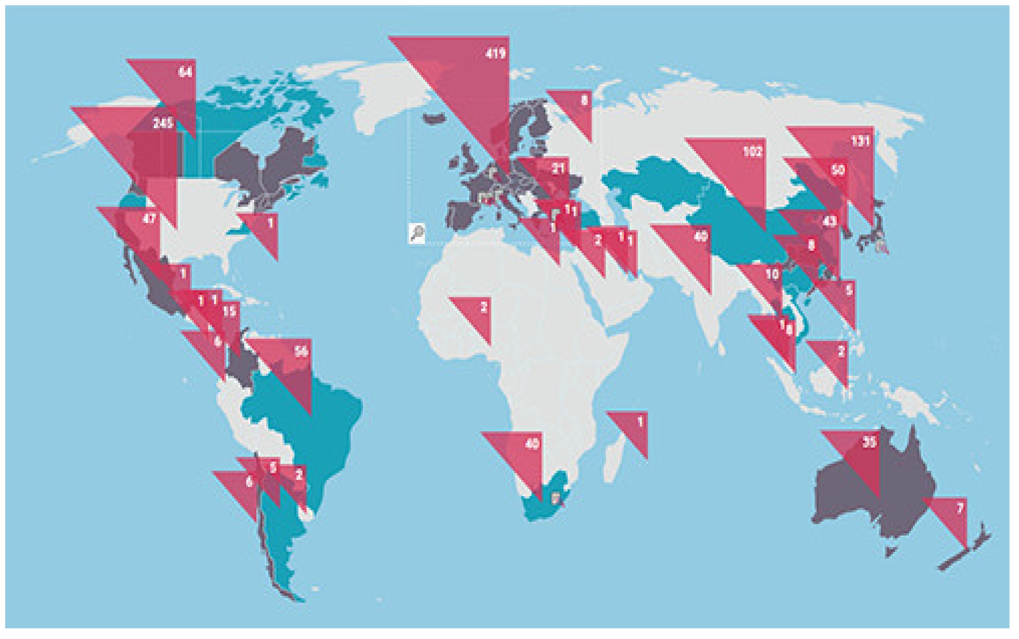
Carbon pricing is an instrument that captures the external costs of GHG emissions—the costs of emissions that the public pays for such as damage to crops, health care costs from heat waves and droughts, and loss of property from flooding and sea level rise—and ties them to their sources through a price, usually in the form of a price on the CO2 emitted (https://carbonpricingdashboard.worldbank.org/what-carbon-pricing, accessed on 30 June 2022). Global carbon pricing revenue in 2021 increased by almost 60% from 2020 levels, to around 84 billion US dollars, providing an important source of funds to help support a sustainable economic recovery, finance broader fiscal reforms, or invest in communities as part of a low-carbon transition future (World Bank, 2022 [27]). Among the types of carbon pricing methods, including carbon taxes (CTs), emissions trading systems (ETS), offsets, and results-based financing (RBF), most advanced countries mainly adopt two ways to price carbon: CT and ETS. According to Carbon Disclosure Project (CDP) statistics, there are 61 carbon pricing mechanisms in the world including 30 CTs and 31 carbon ETSs. Figure 1 shows that the world’s current 64 carbon pricing mechanisms cover 45 countries and 35 states or provinces, accounting for 21.5% of total global GHG emissions (World Bank, 2022 [27]).
In addition, CT refers to the taxation measures offered by the government for large carbon emitters, and the price is determined by the government, for example, CBAM, which will be adopted by the EU in 2023. On the other hand, the ETS is a market mechanism to create more “carbon value” by setting the cap, quota, trading, and flow of carbon emission rights. Furthermore, the price of CT or ETS varies greatly from place to place. For example, Sweden’s carbon tax in 2021 was USD 137/tCO2e, the highest in the world. The amount of Sweden’s carbon tax was 45.7 times that of Japan’s carbon tax (USD 3/tCO2e) during the same period. In 2021, Switzerland’s carbon tax was USD 101/tCO2e, France’s was USD 52/tCO2e, and Singapore’s was USD 4/tCO2e. Later, Taiwan would also impose a carbon tax in the preliminary review of the Climate Change Response Act in 2022, which was also approximately USD 3/tCO2e. The following figure (Figure 2) shows the carbon prices. It can be seen that most carbon prices in 2020 fell in the range of USD 40–80/tCO2e.

2.2. GHGs and Economic Growth

GDP growth is one of the primary macroeconomic factors for a country’s policymaking, as reaching a desired growth rate is considered a main economic objective. However, ecological and environmental costs cannot be ignored. Therefore, the linkage of economic growth and CO2 emissions has gained the attention of policymakers, practitioners, and researchers in recent times (Bashir et al., 2020 [26]).
To investigate the relationship between environmental degradation and economic growth, Grossman and Krueger (1991) [28] and Selden and Song (1994) [29] were among the pioneer researchers to imply that economic growth contributes to environmental degradation initially, and after reaching a certain economic threshold, environmental quality improves. However, the findings of Bashir et al., (2020) [26] suggest that CO2 emissions increase in parallel with economic growth, which contradicts the former studies.
Furthermore, the environmental Kuznets curve (EKC) is a milestone hypothesized relationship among various indicators of environmental degradation and per capita income proposed by Kuznets (1955) [30]. According to Kuznets (1955) [30], the economic development of a country has an inverted U-shaped relationship with its environmental degradation index. That is, in the process of economic development, environmental degradation will increase due to the exploitation of natural resources or the use of industrial equipment. However, when economic development reaches a certain level, the degree of degradation of the environment will decrease due to the fact of R&D of processes or the relocation of manufacturing departments, or even improvement in domestic environmental awareness. In short, the EKC hypothesis states that “the solution to pollution is economic growth”. As a result, the model of EKC is given as follows:
ln E n , t = β n , 0 + β n , 1 · ln Y n , t + β n , 2 · ln Y n , t 2
where, E n , t is the indicator of environmental degradation, Y n , t is the nth country’s income per capita in t years. In Kuznets’ results, the coefficient of linear term β n , 1 > 0 and the coefficient of quadratic term β n , 2 < 0 . As a result, the relationship between the environmental indicator and national income per capita is an inverted U-shaped curve as shown in the following figure.
According to the inverted U-shaped curve in Figure 3, there is a per capita income level Y*, so that when the per capita income does not reach Y*, the environmental degradation index will increase with the increase of the per capita income level. When the per capita income exceeds Y*, the environmental degradation index will decrease with the increase of the per capita income level.
In summary, there are many researches in studying the relationship linking the carbon dioxide emissions to economic growth from 2013 on. Some researches investigate the EKC hypothesis by using a single-country data, for instance, Shahbaz et at. (2013) [32] for Romania, Wang et al., (2016) [10] and Sun et al., (2021) [33] for China, Ahmad et al., (2017) [34] for Croatia, Bekhet and Othman (2018) [35] for Malaysia, Uzar and Eyuboglu (2019) [36] for Turkey, and Koc and Bulus (2020) [37] for South Korea.
Moreover, some researches investigate it by using regional data. For example, Salahuddin and Gow (2014) [38] for GCC countries, Lin et al., (2016) [39] for 5 African countries, Lu (2017) [40] for 16 Asian countries, Mensah et al., (2019) [41] for 22 African countries, Balsalobre-Lorente, and Leitão (2020) [35] for 28 EU countries, and Aslan, Altinoz, and Özsolak (2021) [42] for Mediterranean countries. In addition, some other researches test the EKC hypothesis by using some major countries, such as Azam et al., (2016) [43] for USA, China India and Japan; Bashir et al., (2020) [26] and Dogru et al., (2020) [44] for OECD economies; Kongkuah et al., (2021) [45] for Belt and Road countries and OECD economies. Their empirical results are shown in the following table (Table 4).
Such that, if the EKC hypothesis holds, then the annual amount of CO2 emission equivalent, Q t is an inverted U-shaped function of national income per capita. Therefore, we have,
Δ Q t Q t 1 = b 1 + 2 · b 2 · ln Y t 1 · Δ Y t Y t 1
It means that the change of the amount of CO2 emissions is correlated to the rate of economic growth.

3. The Model

3.1. Optimal Allocation with Economic Growth

Suppose the rate of economic growth for economy n is defined by
R n , t Δ G D P n , t G D P n , t 1 × 100 = Δ GDP   per   Capita n , t GDP   per   Capita n , t 1 × 100
then the average of the rate of economic growth (sample mean) is
R ¯ n 1 T · t = 1 T R n , t = J T · J T 1 · J T · R
where, R be the vector of the economic growth rate of the N economies and J T is the ones vector in T . In addition, the volatility of the rate of economic growth (sample variance) is given as follows:
σ n = 1 T 1 · t = 1 T R n , t R ¯ n 2
Next, the covariance matrix can be found as follows:
Σ V a r R = σ k , m M N × N
where, σ k , m 1 T 1 · t = 1 T R k , t R ¯ k · R m , t R ¯ m is the sample covariance of R k and R m .
Furthermore, assume that w n is the share of global economic growth of the nth economy, then the rate of the global economic growth is the weighted average of economic growth rate of all economies, that is,
R G = n = 1 N w n · R ¯ n = W · R
where W = w 1 , w 2 , , w N N . In addition, the volatility of the global economic growth is
Σ G V a r W · R = W · Σ · W
Such that, an optimal share for each economy is to minimize the volatility of the global economic growth subject to a lower bound of global economic growth. In other words, the mathematical model is given by
min W 1 2 · Σ G = 1 2 · W · Σ · W
s . t .   W · R μ 0
J N · W = 1
where, J N is the ones vector in N and μ 0 is a pre-specified growth rate. Using the Lagrange multipliers method (See Markowitz (1952) [23], Merton (1972) [47], Jang and Chen (2008) [48], Chen, Jang, and Peng (2010) [24], and Hsiao (2017) [25]), we have,
W * A r g min W 1 2 · Σ G = λ 1 · Σ 1 · R + λ 2 · Σ 1 · J N
where, λ 1 = 1 D · C · μ 0 B and λ 2 = 1 D · A B · μ 0 . In addition, A = R · Σ 1 · R , B = J N · Σ 1 · R , C = J N · Σ 1 · J N , and D = A · C B 2 .
As shown in Hsiao (2017) [25], the expected global economic growth rate is
R G * = W * · R = λ 1 · Σ 1 · R + λ 2 · Σ 1 · J N · R = μ 0
and the volatility of change of the amount of CO2 emission is
V a r R G * = W * · Σ · W * = C D · μ 0 B C 2 + 1 C σ G * 2
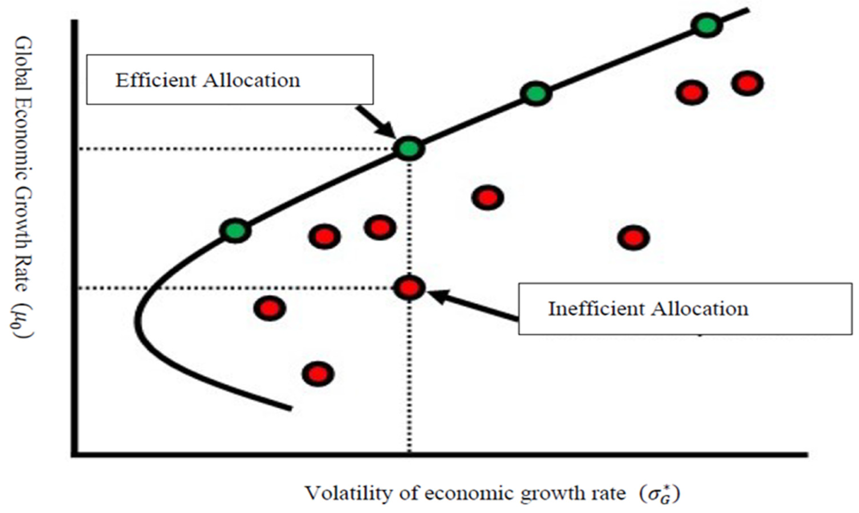
Hence, the relationship between the volatility of the economic growth rate σ G * and global economic growth μ 0 is a hyperbola shown in the following figure (Figure 4).

3.2. Optimal Allocation with CO2 Emissions

Hereinafter, assuming that the EKC hypothesis does hold, that is, the Equation (2) can be rewritten as follows:
E M n , t = b n , 1 + 2 · b n , 2 · ln GDP   per   Capita n , t 1 · R n , t
where, E M n , t Δ Q n , t Q n , t 1 × 100 , is the annual rate of change of CO2 emissions of the nth country in the tth year.
Next, by letting
K n b n , 1 + 2 b n , 2 · ln GDP   per   Capita n , 0 , , b n , 1 + 2 b n , 2 · ln GDP   per   Capita n , T 1
then, we have, E M n , t = K n · R n , t and
E M ¯ n 1 T · t = 1 T E M n , t = J T · J T 1 · J T · K n · R n , t
Moreover, let K Diag K 1 , K 2 , , K N , an N × N diagonal matrix, then the
E M E ¯ 1 , E ¯ 2 , , E ¯ N = J T · J T 1 · J T · K · R .
In addition, the covariance matrix
V a r E M = V a r J T · J T 1 · J T · K · R = J T · J T 1 · J T · K · Σ · K · J T · J T · J T 1
As a result, the optimal allocation with CO2 emissions is given as follows:
W E * = W * · K 1
where, W * is given by the Equation (12).
Hence, the global growth rate of CO2 emission with the optimal allocation is given as follows:
E M G * = W E * · E M = W * · K 1 · K · R = W * · R = μ 0 .
And, the volatility of the global growth rate of CO2 emission can be found by
V a r E M G * = V a r W E * · E M = C D · μ 0 B C 2 + 1 C = σ G * 2
Furthermore, the optimal quota of CO2 emission for the country n in the next year is given as follows:
Q n , t + 1 * = Q n , t · 1 + μ 0 · e n · W E *
where, e n is the nth column vector of an N × N identity matrix.

4. Empirical Evidence

4.1. Data

This study collects the global CO2 emission from the database of Global Carbon Project (https://www.globalcarbonproject.org/carbonbudget/21/data.htm, accessed on 10 May 2022), s and GDP per capita is from World Bank (https://data.worldbank.org/indicator/NY.GDP.PCAP.CD, accessed on 10 May 2022), respectively. Moreover, Taiwan’s macroeconomic data is downloaded from Republic of China (Taiwan) National Statistics (https://eng.stat.gov.tw/point.asp?index=1, accessed on 12 May 2022). Then the descriptive statistics for the variables are shown in the following table (Table 5).

4.2. Test for EKC Hypothesis

On the other hand, the database of Our Data in World collects more comprehensive country-level data including CO2 emission and macroeconomic data, for instance, population, population density, etc. Excluding the countries with incomplete data, this study collects a total of 3402 country-year data from Our World in Data database.
To test the EKC hypothesis for each country, the model:
ln C O 2 e t o n i , t = b i , 0 + b i , 1 · ln GDP   per   Capita i , t + b i , 2 · ln GDP   per   Capita i , t 2 + ε i , t
where, C O 2 e t o n i , t , the dependent variable, is the CO2 emission equivalent in million tons of weight and GDP   per   Capita i , t , the independent variable, is the annual GDP per capita in thousands of US dollars of country i in t year. ε i , t is a disturbance term with mean zero and constant variance σ ε , i 2 . Such that, the null hypothesis and alternative hypothesis are
H 0 :   b n , 2 < 0   versus   to   H 1 :   b n , 2 0
The test results are shown in the following table (Table 6).
As shown in Table 6, it can be seen that most of countries in Europe, North America, South America, and Oceania, support to the EKC hypothesis, however, there are almost half of countries in Asia and Africa which are not supported to the EKC hypothesis. On the other hand, some countries either in Europe or in Asia which support to the EKC hypothesis, however, the estimates of quadratic term are insignificant.

4.3. Computation of Optimal Allocation of CO2 Emission Quota

The first step is to calculate the optimal allocation with economic growth, W * by using the Equation (12). Second, in accordance to the Equation (24), estimate the regression coefficients of b’s for each country. Third, the diagonal matrix, K, was formed, and then the optimal allocation of a CO2 emissions quota was determined by W E * , given in Equation (19). Such that, the optimal CO2 emission quota considering the economic growth can be found by Equation (22).

4.3.1. Continental Economics and CO2 Emissions

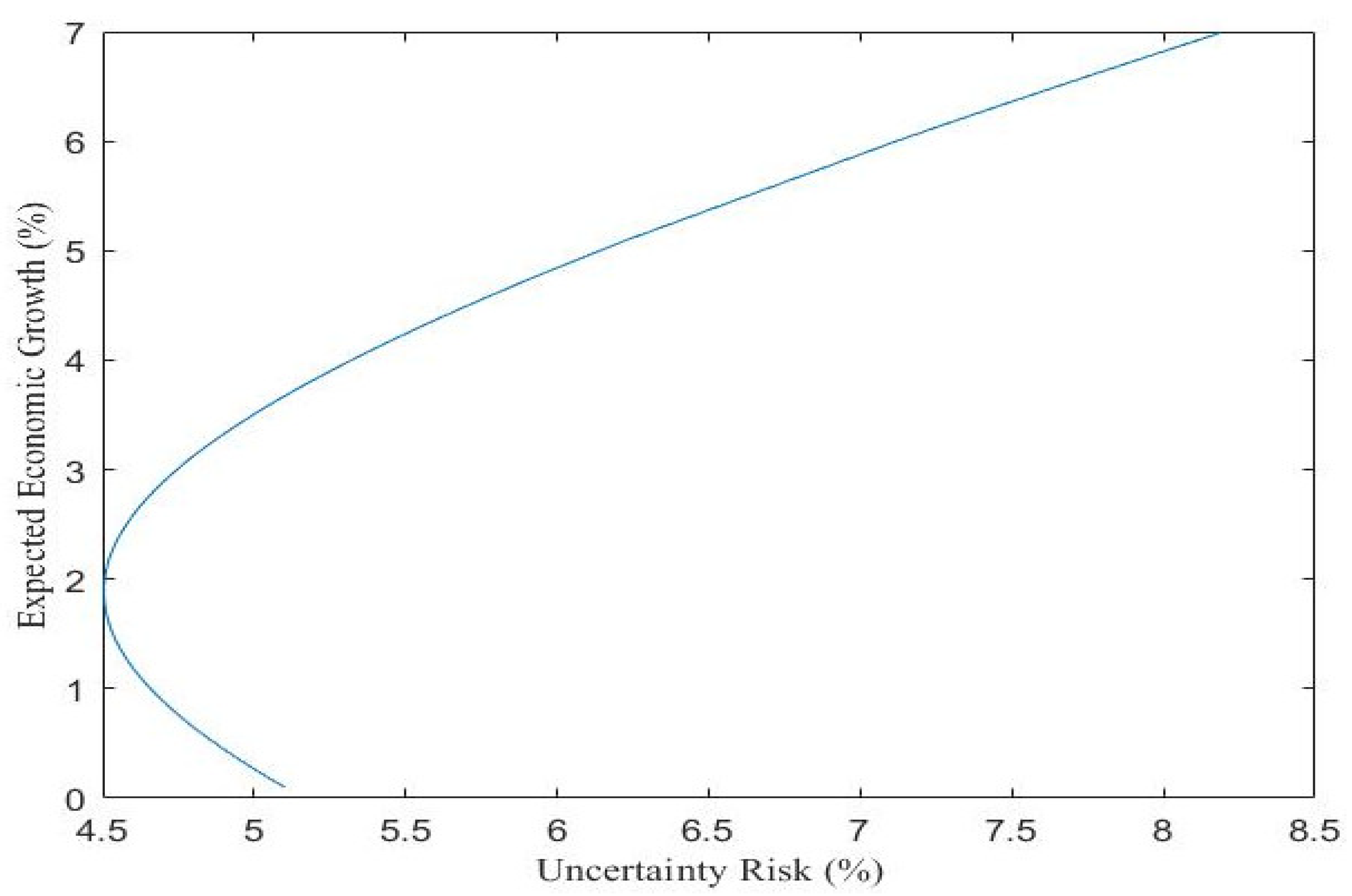
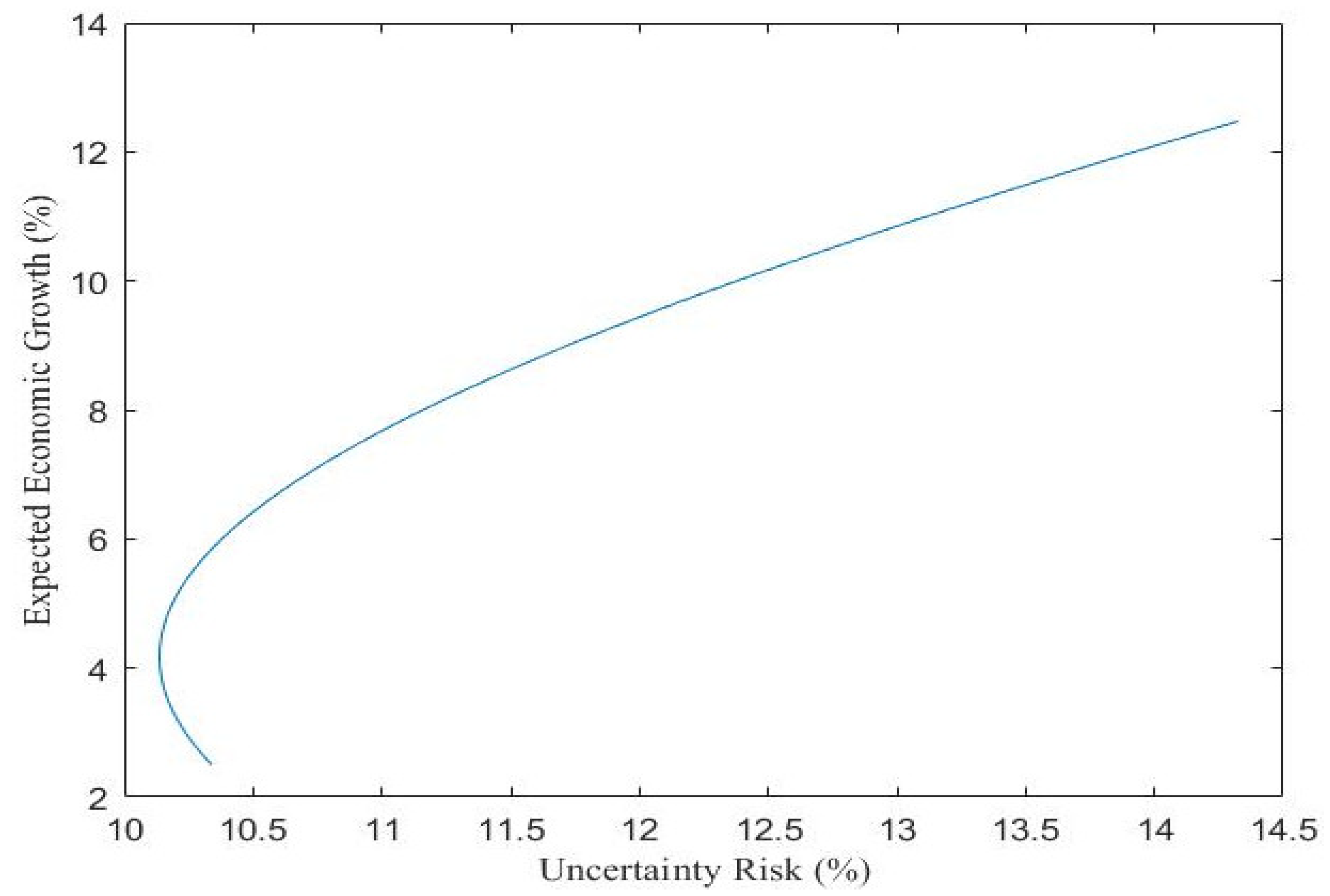
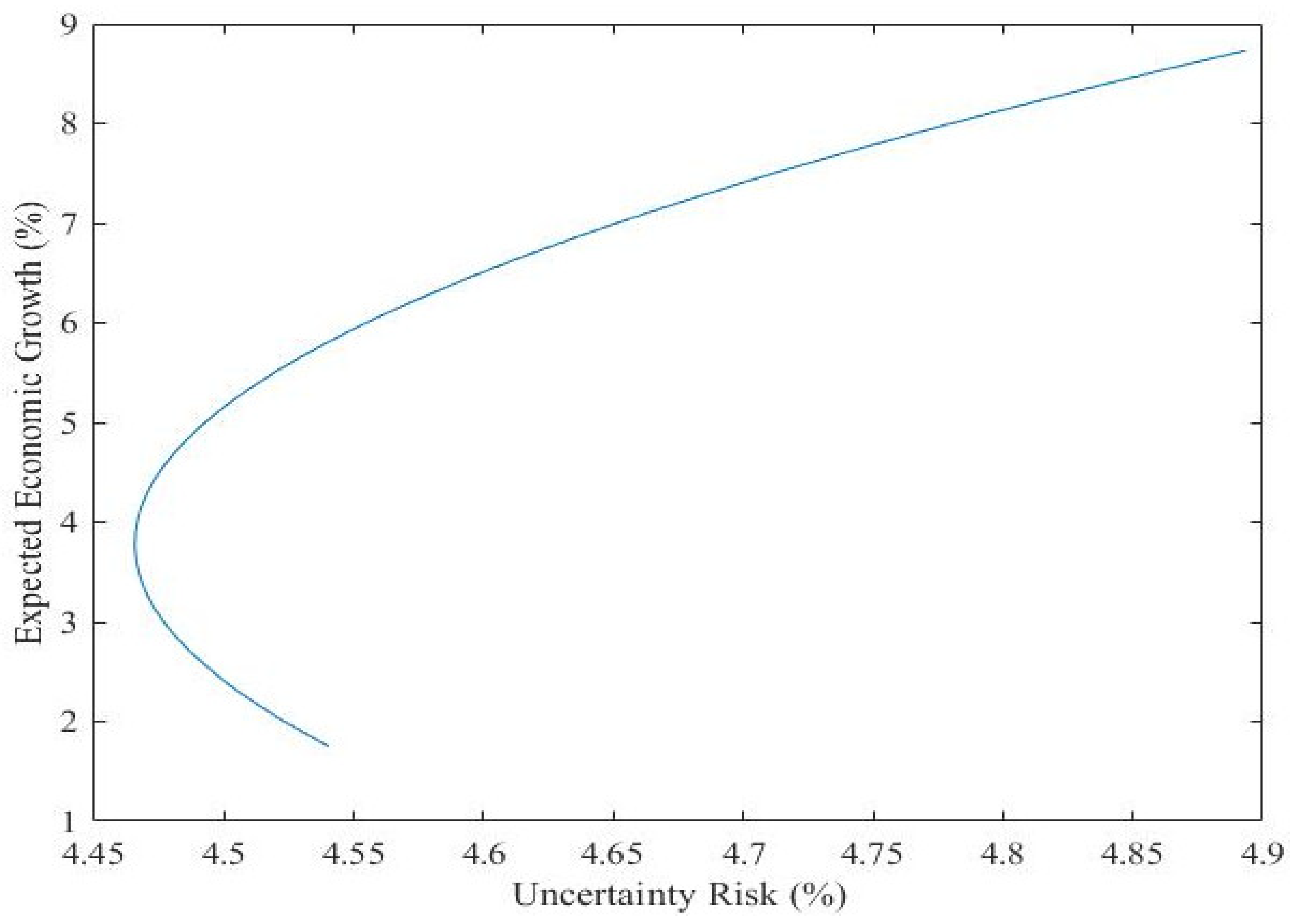
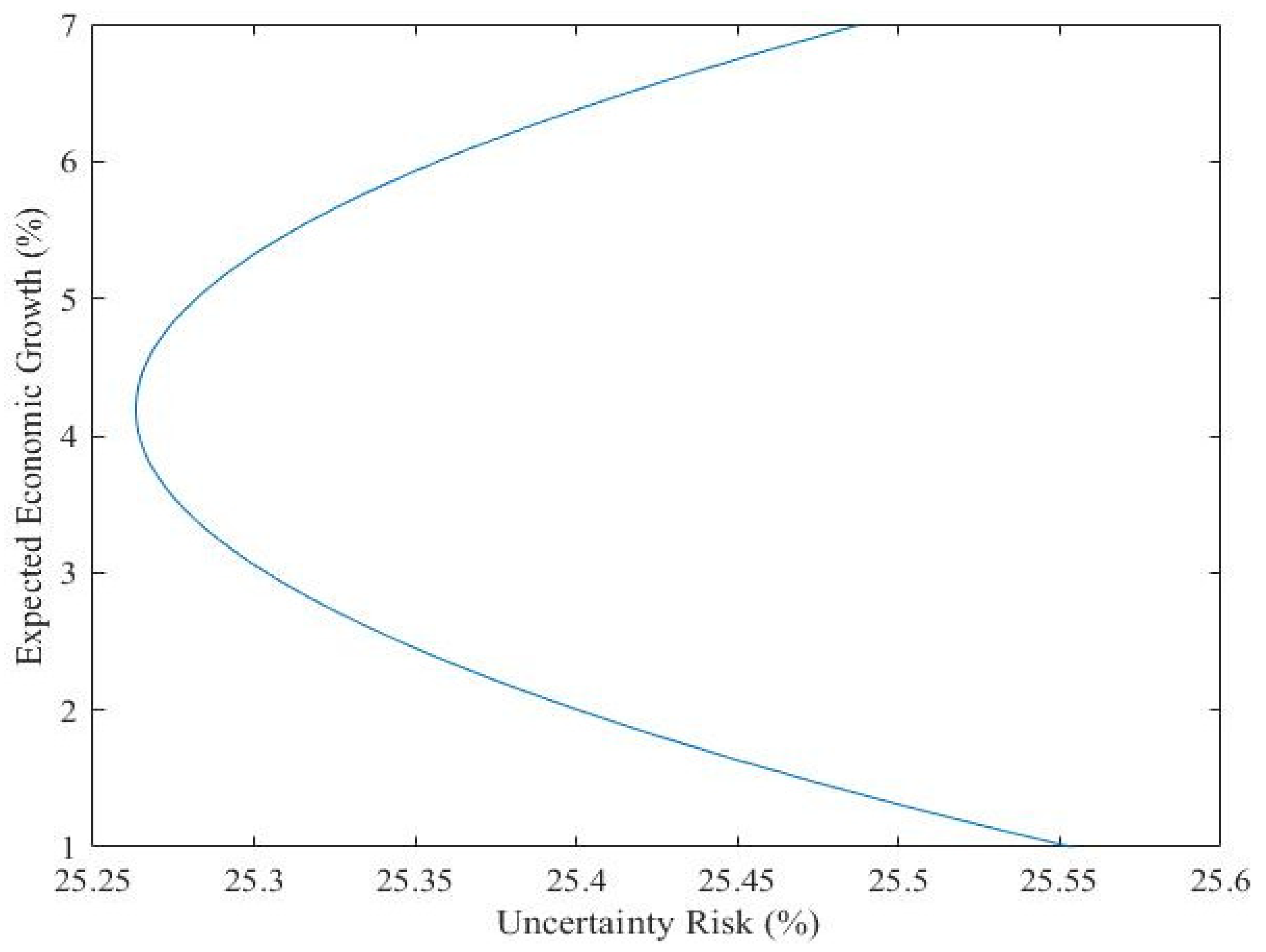
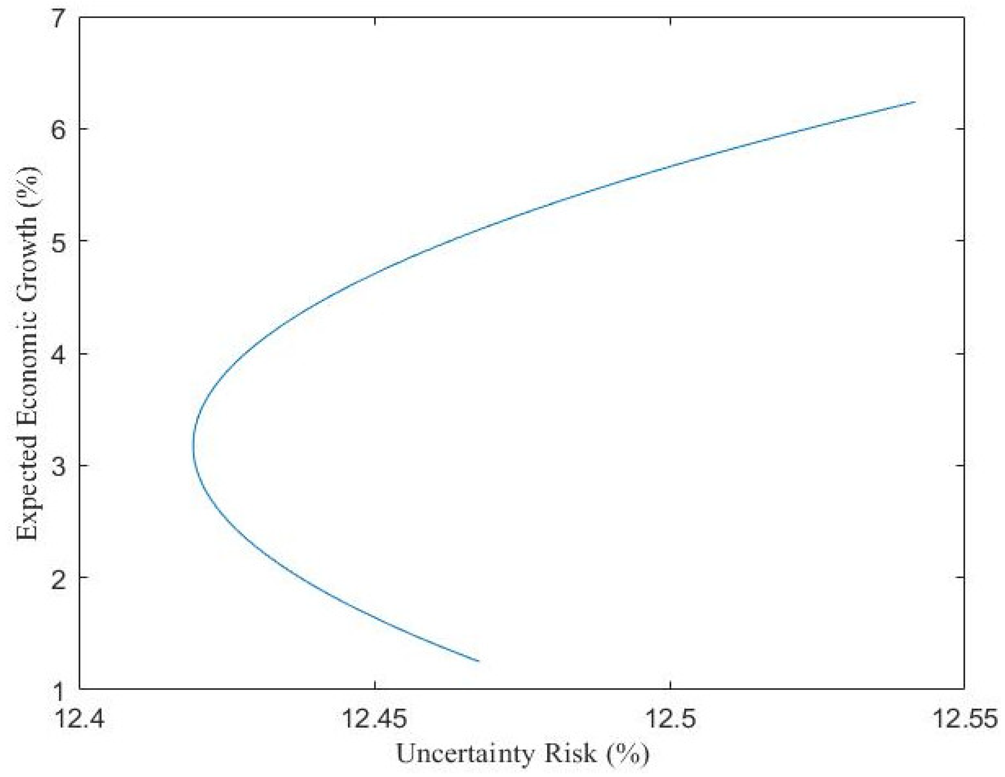
For each continent, countries’ CO2 emission and GDP per capita have been collected from the Our World in Data website for the last 20 years. The efficiency frontier curve of the optimal allocation of CO2 emissions in countries with a minimum risk of economic growth uncertainty are shown in Figure 5, Figure 6, Figure 7, Figure 8 and Figure 9.
As shown in the Figure 5, Figure 6, Figure 7, Figure 8 and Figure 9, the higher the expected economic growth rate, the higher the uncertainty risk. The Asian regional economic growth is the less volatile than other continents, however the African regional economic growth has the highest volatility. It may be contributed to the larger difference of economic condition between the African countries than that in the other continents.

4.3.2. Global Economics and CO2 Emissions

As for the global economic, data on a total of 162 countries were collected from the Our World in Data website for the last 20 years. The efficiency front curve of the optimal allocation of CO2 emissions in countries with the minimum risk of global economic growth uncertainty (see Figure 10). As shown in the Figure 10, the higher the expected economic growth rate, the higher the uncertainty risk. For instance, if the global expected economic growth rate of 6%, then the uncertainty risk was approximately 12.52%; however, if the global expected economic growth rate was of 12%, then the uncertainty risk was approximately 20.63%. Therefore, under this situation, the amount of CO2 emissions of global countries are shown in the following table.
Since this study uses the emissions of the previous year as the benchmark when estimating GHG emissions in the following year, according to the proportion of global economic growth that countries should bear, since 2020 onwards, due to the closure of borders and the reduction of economic activities due to the COVID-19 lockdown, the economies of various countries have come to a standstill (Le Quéré et al., 2020 [3]; Hsiao, 2022 [4]); thus, their GHG emissions have also greatly reduced. Therefore, the GHG emission amounts of each country in the following year will be lower than those before 2020.
The results in Table 7 show that the optimal quota of CO2 emissions may decrease compared to the amount in the previous year, considering the uncertainty risk of global economic growth (volatility) for some countries, especially for larger economies in Europe or North America and smaller economies in Africa. However, there are some countries that may increase their amount of CO2 emissions when considering global economic growth such as the larger economies in Asia or Africa.
Table 7 also reveals that not all countries should take carbon reduction actions immediately. Under the consideration of global economic growth, countries have their own economic growth needs and carry out appropriate economic activities. When the EKC hypothesis holds, economic activities may degrade the environmental index; however, they may also improve the quality of the environment such as the improvement in production technology, the development of environmental protection equipment, the increase in green financial investment, and technological innovation of carbon sequestration or carbon capture. As a result, some over-emitting countries should formulate policies to reduce emissions and achieve their commitments to COP26. According to US EPA research, there are many ways that governments can promote carbon reduction programs such as improving energy efficiency, increasing energy conservation subsidies, replacing fossil energy with renewable energy, promoting carbon sequestration or carbon capture technology research and development, and changing land use and management. Furthermore, under-emitting countries may take appropriate economic activities to improve their economic growth level, which will help world economic growth, although it will increase GHG emissions. In addition, part of their carbon rights can be traded with other countries that emit excess emissions through the international carbon rights trading platforms.

5. Concluding Remarks

In this study, the linkage between CO2 emission equivalents and GDP per capita is an inverted U-shaped function for most countries that support the EKC hypothesis. Under the EKC hypothesis, this study proposed a framework to determine an optimal allocation of CO2 emissions for each country considering global economic growth and uncertainty risk. Based on this allocation, government policymakers may implement policies to reduce extra emissions such as energy efficiency and energy conservation enhancement, fuel switching, carbon capture and sequestration, and land management practices.
Furthermore, the framework proposed in this study can be applied to industry-level data and even company-level data in addition to national-level data. It is said that under the premise of considering the national economic growth, the optimum GHG emissions/sinks of each industry or company should be calculated to minimize the uncertainty risk, first, and then policies should be formulated to improve GHG emissions/sinks of each industry or company.

Funding

This research received no external funding.

Institutional Review Board Statement

Not applicable.

Informed Consent Statement

Not applicable.

Data Availability Statement

Not applicable.

Conflicts of Interest

The author declares no conflict of interest.

References

  1. Guggenheim, P.D.; Al Gore, A.A. An Inconvenient Truth; Paramount Pictures Corporation: Los Angeles, CA, USA, 2006. [Google Scholar]
  2. TVBS Sisy’s World News Group. ±2 °C—The Truth That Taiwan Must Face; Taiwan, 2010; Available online: https://movie.douban.com/subject/4312211/ (accessed on 16 May 2022).
  3. Le Quéré, C.; Jackson, R.B.; Jones, M.W.; Smith, A.J.; Abernethy, S.; Andrew, R.M.; De-Gol, A.J.; Willis, D.R.; Shan, Y.L.; Canadell, J.G.; et al. Temporary Reduction in Daily Global CO2 Emissions during the COVID-19 Forced Confinement. Nat. Clim. Change 2020, 10, 647–653. [Google Scholar] [CrossRef]
  4. Hsiao, C.M. Effects on Second Waves of COVID-19 Epidemics: Social Stringency, Economic Forces, and Public Health. Theor. Econ. Lett. 2022, 12, 278–320. [Google Scholar] [CrossRef]
  5. Abbass, K.; Qasim, M.Z.; Song, H.M.; Murshed, M.; Mahmood, H.; Younis, I. A Review of the Global Climate Change Impacts, Adaptation, and Sustainable Mitigation Measures. Environ. Sci. Pollut. Res. 2022, 29, 42539–42559. [Google Scholar] [CrossRef] [PubMed]
  6. Forster, P.; Storelymo, T.; Armour, K.; Collins, W.; Dufresne, J.; Frame, D.; Lunt, D.; Mauritsen, T.; Palmer, M.; Watanabe, M.; et al. Chapter 7: The Earth’s Energy Budget, Climate Feedbacks, and Climate Sensitivity. In Climate Change 2021: The Physical Science Basis; Contribution of Working Group I to the Sixth Assessment Report of the Intergovernmental Panel on Climate Change; IPCC: Geneva, Switzerland, 2021; Available online: https://www.ipcc.ch/report/ar6/wg1/downloads/report/IPCC_AR6_WGI_FOD_Chapter07.pdf (accessed on 16 May 2022).
  7. Myhre, G.; Shindell, D.; Bréon, F.M.; Collins, W.; Fuglestvedt, J.; Huang, J.; Koch, D.; Lamarque, J.-F.; Lee, D.; Mendoza, B.; et al. Chapter 8: Anthropogenic and Natural Radiative Forcing. In Climate Change 2013: The Physical Science Basis; Contribution of Working Group I to the Fifth Assessment Report of the Intergovernmental Panel on Climate Change; IPCC: Geneva, Switzerland, 2013; pp. 659–740. Available online: https://archive.ipcc.ch/pdf/assessment-report/ar5/wg1/WG1AR5_Chapter08_FINAL.pdf (accessed on 16 May 2022).
  8. Golombek, R.; Kittelsen, S.A.C.; Rosendahl, K.E. Price and Welfare Effects of Emission Quota Allocation. Energy Econ. 2013, 36, 568–580. [Google Scholar] [CrossRef] [Green Version]
  9. Zhou, P.; Zhang, L.; Zhou, D.Q.; Xia, W.J. Modeling Economic Performance of Interprovincial CO2 Emission Reduction Quota Trading in China. Appl. Energy 2013, 112, 1518–1528. [Google Scholar] [CrossRef]
  10. Wei, Y.M.; Wang, L.; Liao, H.; Wang, K.; Murty, T.; Yan, J.Y. Responsibility Accounting in Carbon Allocation: A Global Perspective. Appl. Energy 2014, 130, 122–133. [Google Scholar] [CrossRef]
  11. Pan, X.Z.; Teng, F.; Wang, G.H. A Comparison of Carbon Allocation Schemes: On the Equity-Efficiency Tradeoff. Energy 2014, 74, 222–229. [Google Scholar] [CrossRef]
  12. Pan, X.Z.; Teng, F.; Wang, G.H. Sharing Emission Space at an Equitable Basis: Allocation Scheme based on the Equal Cumulative Emission per Capita Principle. Appl. Energy 2014, 113, 1810–1818. [Google Scholar] [CrossRef]
  13. Zhang, Y.J.; Wang, A.D.; Da, Y.B. Regional Allocation of Carbon Emission Quotas in China: Evidence from the Shapley Value Method. Energy Policy 2014, 74, 454–464. [Google Scholar] [CrossRef]
  14. Hao, Y.; Liao, H.; Wei, Y.M. Is China’s Carbon Reduction Target Allocation Reasonable? An Analysis based on Carbon Intensity Convergence. Appl. Energy 2015, 142, 229–239. [Google Scholar] [CrossRef]
  15. Pang, R.Z.; Deng, Z.Q.; Chiu, Y.H. Pareto Improvement through a Reallocation of Carbon Emission Quotas. Renew. Sustain. Energy Rev. 2015, 50, 419–430. [Google Scholar] [CrossRef]
  16. Carretero, A.L.; de la Rosa, J.; Sanchez-Rodas, D. Applying Statistical Tools Systematically to Determine Industrial Emission Levels associated with the best Available Techniques. J. Clean. Prod. 2016, 112, 4226–4236. [Google Scholar] [CrossRef]
  17. Miao, Z.A.; Geng, Y.; Sheng, J.C. Efficient Allocation of CO2 Emissions in China: A Zero Sum Gains Data Envelopment Model. J. Clean. Prod. 2016, 112, 4144–4150. [Google Scholar] [CrossRef]
  18. Han, R.; Tang, B.J.; Fan, J.L.; Liu, L.C.; Wei, Y.M. Integrated Weighting Approach to Carbon Emission Quotas: An Application Case of Beijing-Tianjin-Hebei Region. J. Clean. Prod. 2016, 131, 448–459. [Google Scholar] [CrossRef]
  19. Chang, K.; Zhang, C.; Chang, H. Emissions Reduction Allocation and Economic Welfare Estimation through Interregional Emissions Trading in China: Evidence from Efficiency and Equity. Energy 2016, 113, 1125–1135. [Google Scholar] [CrossRef]
  20. An, Q.X.; Wen, Y.; Xiong, B.B.; Yang, M.; Chen, X.H. Allocation of Carbon Dioxide Emission Permits with the Minimum Cost for Chinese Provinces in Big Data Environment. J. Clean. Prod. 2017, 142, 886–893. [Google Scholar] [CrossRef]
  21. Zhou, Z.B.; Liu, C.J.; Zeng, X.M.; Jiang, Y.J.; Liu, W.B. Carbon Emission Performance Evaluation and Allocation in Chinese Cities. J. Clean. Prod. 2018, 172, 1254–1272. [Google Scholar] [CrossRef]
  22. Crémieux, L. What Is at Stake in the “Yellow Jacket” Mobilization. International Viewpoint. 2018. Available online: https://internationalviewpoint.org/IMG/pdf/what-is-at-stake-in-the-yellow-jacket-mobilization_a5802.pdf (accessed on 27 November 2018).
  23. Markowitz, H. Portfolio Selection. J. Financ. 1952, 7, 77–91. [Google Scholar]
  24. Chen, M.H.; Jang, S.C.; Peng, Y.J. Discovering Optimal Tourist Market Mixes. J. Travel Res. 2010, 50, 602–614. [Google Scholar] [CrossRef]
  25. Hsiao, C.M. Enterprise Risk Management with Foreign Exchange Exposures: Evidence from Taiwan Tourism Industry. Asian Econ. Financ. Rev. 2017, 7, 882–906. [Google Scholar]
  26. Bashir, M.F.; Ma, B.J.; Shahbaz, M.; Jiao, Z.L. The Nexus between Environmental Tax and Carbon Emissions with the Roles of Environmental Technology and Financial Development. PLoS ONE 2020, 15, e0242412. [Google Scholar] [CrossRef]
  27. World Bank. State and Trends of Carbon Pricing 2021; World Bank: Washington, DC, USA, 2021; p. 10. [Google Scholar] [CrossRef]
  28. Grossman, G.M.; Krueger, A.B. Environmental Impacts of a North American Free Trade Agreement. In National Bureau of Economic Research Working Paper, No. 3914; National Bureau of Economic Research: Cambridge, MA, USA, 1991. [Google Scholar]
  29. Selden, T.M.; Song, D. Environmental Quality and Development: Is there a Kuznets curve for Air Pollution Emissions? J. Environ. Econ. Manag. 1994, 27, 147–162. [Google Scholar] [CrossRef]
  30. Kuznets, S. Economic Growth and Income Inequality. Am. Econ. Rev. 1955, 45, 1–28. [Google Scholar]
  31. Stern, D.I.; Common, M.S.; Barbier, E.B. Economic Growth and Environmental Degradation: The Environmental Kuznets Curve and Sustainable Development. World Dev. 1996, 24, 1151–1160. [Google Scholar] [CrossRef]
  32. Shahbaz, M.; Mutascu, M.; Azim, P. Environmental Kuznets Curve in Romania and the Role of Energy Consumption. Renew. Sustain. Energy Rev. 2013, 18, 165–173. [Google Scholar] [CrossRef] [Green Version]
  33. Sun, Y.; Li, M.X.; Zhang, M.J.; Khan, H.S.U.; Li, J.Q.; Li, Z.Y.; Sun, H.Z.; Zhu, Y.; Anaba, O.A. A Study on China’s Economic Growth, Green Energy Technology, and Carbon Emissions based on the Kuznets curve (EKC). Environ. Sci. Pollut. Res. 2021, 28, 7200–7211. [Google Scholar] [CrossRef]
  34. Ahmad, N.; Du, L.S.; Lu, J.Y.; Wang, J.L.; Li, H.Z.; Hashmi, M.Z. Modelling the CO2 Emissions and Economic Growth in Croatia: Is there any Environmental Kuznets Curve? Energy 2017, 123, 164–172. [Google Scholar] [CrossRef]
  35. Balsalobre-Lorente, D.; Leitão, N.C. The Role of Tourism, Trade, Renewable Energy Use and Carbon Dioxide Emissions on Economic Growth: Evidence of Tourism-led Growth Hypothesis in EU-28. Environ. Sci. Pollut. Res. 2020, 27, 45883–45896. [Google Scholar] [CrossRef]
  36. Uzar, U.; Eyuboglu, K. The Nexus between Income Inequality and CO2 Emissions in Turkey. J. Clean. Prod. 2019, 227, 149–157. [Google Scholar] [CrossRef]
  37. Koc, S.; Bulus, G.C. Testing Validity of the EKC Hypothesis in South Korea: Role of Renewable Energy and Trade Openness. Environ. Sci. Pollut. Res. 2020, 27, 29043–29054. [Google Scholar] [CrossRef]
  38. Salahuddin, M.; Gow, J. Economic Growth, Energy Consumption and CO2 Emissions in Gulf Cooperation Council Countries. Energy 2014, 73, 44–58. [Google Scholar] [CrossRef]
  39. Lin, B.Q.; Omoju, O.E.; Nwakeze, N.M.; Okonkwo, J.U.; Megbowon, E.T. Is the Environmental Kuznets Curve Hypothesis a Sound Basis for Environmental Policy in Africa? J. Clean. Prod. 2016, 133, 712–724. [Google Scholar] [CrossRef]
  40. Lu, W.C. Greenhouse Gas Emissions, Energy Consumption and Economic Growth: A Panel Cointegration Analysis for 16 Asian Countries. Int. J. Environ. Res. Public Health 2017, 14, 1436. [Google Scholar] [CrossRef] [Green Version]
  41. Mensah, I.A.; Sun, M.; Gao, C.X.; Omari-Sasu, A.Y.; Zhu, D.B.; Ampimah, B.C.; Quarcoo, A. Analysis on the Nexus of Economic Growth, Fossil Fuel Energy Consumption, CO2 Emissions and Oil Price in Africa based on a PMG Panel ARDL Approach. J. Clean. Prod. 2019, 228, 161–174. [Google Scholar] [CrossRef]
  42. Aslan, A.; Altinoz, B.; Özsolak, B. The Nexus between Economic Growth, Tourism Development, Energy Consumption, and CO2 Emissions in Mediterranean Countries. Environ. Sci. Pollut. Res. 2021, 28, 3243–3252. [Google Scholar] [CrossRef] [PubMed]
  43. Azam, M.; Khan, A.Q.; Abdullah, H.B.; Qureshi, M.E. The Impact of CO2 Emissions on Economic Growth: Evidence from Selected Higher CO2 Emissions Economies. Environ. Sci. Polluti. Res. 2016, 23, 6376–6389. [Google Scholar] [CrossRef] [PubMed]
  44. Dogru, T.; Bulut, U.; Kocak, E.; Isik, C.; Suess, C.; Sirakaya-Turk, E. The Nexus between Tourism, Economic Growth, Renewable Energy Consumption, and Carbon Dioxide Emissions: Contemporary Evidence from OECD Countries. Environ. Sci. Pollut. Res. 2020, 27, 40930–40948. [Google Scholar] [CrossRef]
  45. Kongkuah, M.; Yao, H.X.; Fongjong, B.B.; Agyemang, A.O. The Role of CO2 Emissions and Economic Growth in Energy Consumption: Empirical Evidence from Belt and Road and OECD Countries. Environ. Sci. Pollut. Res. 2021, 28, 22488–22509. [Google Scholar] [CrossRef]
  46. Bekhet, H.A.; Othman, N.S. The Role of Renewable Energy to Validate Dynamic Interaction between CO2 Emissions and GDP toward Sustainable Development in Malaysia. Energy Econ. 2018, 72, 47–61. [Google Scholar] [CrossRef]
  47. Merton, R. An Analytic Derivation of the Efficient Portfolio Frontier. J. Financ. Quant. Anal. 1972, 7, 1851–1872. [Google Scholar] [CrossRef] [Green Version]
  48. Jang, S.C.; Chen, M.H. Financial Portfolio Approach to Optimal Tourist Market Mixes. Tour. Manag. 2008, 29, 761–770. [Google Scholar] [CrossRef] [PubMed]
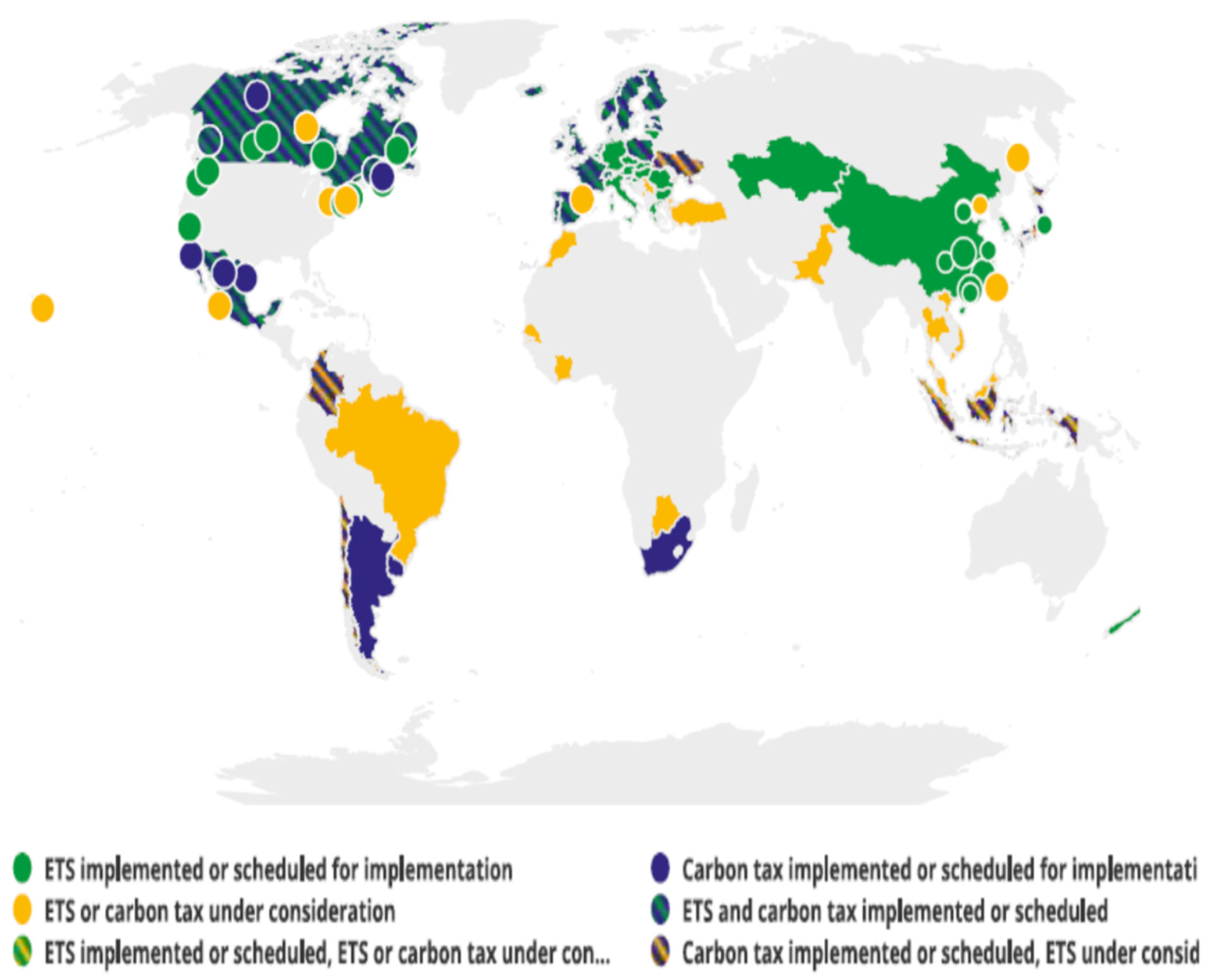
Figure 1. Global carbon pricing mechanisms. Reprinted with permission from Ref. [27]. 2022, World Bank.
Sustainability 14 08706 g001
Figure 2. Carbon prices. Reprinted with permission from Ref. [27]. 2022, World Bank.
Sustainability 14 08706 g002
Figure 3. Environmental Kuznets curve. Source: Stern, Common, and Barbier (1996) [31].
Sustainability 14 08706 g003
Figure 4. Efficient frontier under uncertainty. Source: Hsiao (2017) [25].
Sustainability 14 08706 g004
Figure 5. The efficient frontier of CO2 emission quota for European countries.
Sustainability 14 08706 g005
Figure 6. The efficient frontier of CO2 emission quota for North American countries.
Sustainability 14 08706 g006
Figure 7. The efficient frontier of CO2 emission quota for South American and Oceania countries.
Sustainability 14 08706 g007
Figure 8. The efficient frontier of CO2 emission quota for Asian countries.
Sustainability 14 08706 g008
Figure 9. The efficient frontier of CO2 emission quota for African countries.
Sustainability 14 08706 g009
Figure 10. Efficient frontier of CO2 emission quota for all countries.
Sustainability 14 08706 g010
Table 1. America’s historical top-10 costliest Atlantic hurricanes.
RankNamePressure (mbar)Category (USA)YearDamage (Billion USD)Dead
1Katrina92052005125.01836
2Harvey93742017125.0107
3Maria9205201791.63059
4Irma9145201777.6134
5Ida9294202175.3107
6Sandy9403201268.7233
7Ike9354200838.0214
8Andrew9225199227.365
9Michael9195201825.574
10Florence9274200424.254
Source: United States National Catastrophe Center.
Table 2. Emission sources of GHGs.
GHGMolecular FormulaEmission Sources
Water vaporH2OBoiled water
OzoneO3Light causes O2 to act photochemically.
Carbon dioxideCO2
  • Human burning of fossil fuels
  • Deforestation
  • Biological respiration
MethaneCH4
  • Enteric fermentation (for example, from animal husbandry and cattle raising)
  • Rice
  • Small leakage of fossil fuel transportation
Nitrogen oxidesNO, NO2, N2O, N4O, NO3, N2O3, N2O4, N2O5, N(NO2)3
  • Combustion of biomass
  • Fuel
  • Fertilizer production
ChlorofluorocarbonsChlorofluorocarbons (CFCs)
Hydrochlorofluorocarbons (HCFCs)
Hydrofluorocarbons (HFCs)
Refrigerant escape
PerfluorocarbonsCF4, C2F6, SF6, NF3Insulator
Source: United States Environmental Protection Agency (https://www.epa.gov/ghgemissions/overview-greenhouse-gases, accessed on 16 May 2022).
Table 3. Global warming potential of greenhouse gases.
GHGLifetime (Years)Global Warming Potential (GWP) a
20 Years100 Years500 Years
Carbon dioxide (CO2)20~200111
Methane (CH4)12.482.5327.6
Nitrous oxide (N2O)109273273130
HFC-134a (CH2FCF)1413901526436
CFC-11 (CCl3F)52832162262093
CFC-12 (CCl2F2)10010,80010,2005200
HCFC-22 (CHClF2)1252801760549
Carbon tetrafluoride (CF4, PFC-14)50,0005301738010,587
HFC-32 (CH2F2)52693771220
Hexafluoroethane (C2F6)10,000821011,10018,200
Nitrogen trifluoride (NF3)50012,80019,10020,700
Sulfur hexafluoride (SF6) b320017,50023,50032,600
a It is estimated according to IPCC AR6 WG1 Ch7 2021, contributed by Forster et al., (2021) [6]. b It is estimated according to IPCC AR5 WG1 Ch8 2013, contributed by Myhre et al., (2013) [7]. Source: United States Environmental Protection Agency, 16 May 2022.
Table 4. Researches on the CO2 emission and economic development.
ReferenceStudy Area/PeriodInterpretations
Shahbaz et al., (2013) [32]Romania/1980–2010EKC is found both in long- and short-runs in Romania.
Salahuddin and Gow (2014) [38]GCC countries/1980–2012No significant relationship is found between economic growth and CO2 emissions.
Wang et al., (2016) [10]China/1990–2012Shocks in CO2 emissions has a small effect on energy consumption and GDP.
Azam et al., (2016) [43]USA, China, India, Japan/1971–2013Positive relationship between CO2 emissions and GDP in USA, China and Japan
Lin et al., (2016) [39]Five African countries/1980–2011There is no evidence of the validity of the hypothesis in Africa
Lu (2017) [40]16 Asian countries/1990–2012In the long run, bidirectional Granger causality between energy consumption, GDP and GHG emissions is established.
Ahmad et al., (2017) [34]Croatia/1992Q1–2011Q1.Support to EKC for long-run and bidirectional causality for short-run.
Bekhet and Othman (2018) [46]Malaysia/1971–2015The inverted N-shaped EKC hypothesis holds in Malaysia and the GDP growth will be a remedy for environmental pollution problems.
Uzar and Eyuboglu (2019) [36]Turkey/1984–2014Income inequality has a positive effect on CO2 emissions and the EKC is valid in Turkey.
Mensah et al., (2019) [41]22 African countries/1990–2015A unilateral causality from carbon emissions to economic growth in long-term
Koc and Bulus (2020) [37]South Korea/1971–2017An N-shaped relationship has been identified between per capita CO2 emissions and per capita GDP. This indicates that our empirical findings do not support the EKC hypothesis in South Korea.
Balsalobre-Lorente, and Leitão (2020) [35]EU-28/1995–2014CO2 emissions are positively correlated with economic growth, showing that growth is directly correlated by climate change and GHG.
Bashir et al., (2020) [26]OECD economies/1995–2015Economic growth impedes environmental quality by increasing carbon emissions.
Dogru et al., (2020) [44]OECDTourism development has negative and significant effects on CO2 emission in Canada, Czechia, and Türkiye, while it has positive and significant effects on CO2 emission in Italy, Luxembourg, and the Slovak Republic.
Kongkuah et al., (2021) [45]Belt and Road Countries, OECDBoth CO2 emissions and economic growth positively and significantly affect energy consumption.
Aslan, Altinoz, and Özsolak (2021) [42]Mediterranean countries/1995–2014Energy consumption supports economic growth at low and medium growth levels. Short-run causality test results illustrated that there is bidirectional causality between GDP and CO2 emission.
Sun et al., (2021) [33]China/1990–2017In the long-run, the relationship between economic growth and carbon emissions is inverted U-shaped.
Table 5. Descriptive statistics for variables.
VariableObs.MeanMedianSt. Dev.MinMax
CO2eton
(Mtons)
1582423.25100.931124.671.879528.20
GDP per capita
(1000$)
158224.4118.2022.000.37129.36
Source: Global Carbon Project and World Bank.
Table 6. Test results for the EKC hypothesis for each country.
ContinentSupport to EKC HypothesisReject the EKC Hypothesis
EuropeAlbania (−1.4487 ***) Cape Verde (0.1149)
Austria (−0.4760 ***) Czech (−0.1615)
Belarus (−1.8549 ***)Iceland (0.1237)
Belgium (−0.6850 ***) Moldova (1.8505 ***)
Bulgaria (−1.1135 ***)Slovakia (−0.1639 **)
Bosnia and Herzegovina (−0.3911 ***)Ukraine (0.1406)
Croatia (−0.4024 ***)
Cyprus (−0.4714 ***)
Denmark (−0.8906 ***)
Estonia (−2.5935 **)
Finland (−6750 ***)
France (−0.8296 ***)
Germany (−0.8524 ***)
Greece (−0.7889 ***)
Hungary (−1.0287 ***)
Ireland (−0.4113 ***)
Italy (−0.9941 ***)
Latvia (−2.6530 ***)
Lithuania (−1.9727 ***)
Luxembourg (−0.2095 **)
Malta (−0.1906 ***)
Montenegro (−0.3924 ***)
Netherlands (−0.7989 ***)
North Macedonia (−0.8944 ***)
Norway (−0.6379 ***)
Poland (−0.7666 ***)
Portugal (−0.3138 ***)
Romania (−0.5063 ***)
Russia (−0.9728 ***)
Serbia (−0.5766 ***)
Slovenia (−0.2483 ***)
Spain (−0.9438 ***)
Sweden (−0.8761 ***)
Switzerland (−0.4903 ***)
Turkey (−0.2812 ***)
United Kingdom (−0.9471 ***)
Africa
Algeria (−1.5759 ***)Angola (2.1134 ***)
Botswana (−0.7280 ***)Burkina Faso (−7.0044)
Burundi (−10.1060 **)Chad (1.9051 ***)
Cameroon (−5.7137 ***)Comoros (1.3505 **)
Cent. African Rep. (−2.9990 ***)Congo (0.0227)
Dem. Rep. of Congo (−1.8716 ***)Cote d’Ivoire (−3.9265)
Djibouti (−2.1016 ***)Equatorial Guinea (0.2423 ***)
Egypt (−0.4208 *)Ethiopia (0.9081)
Eswatini (−1.0469 ***)Gambia (0.7366)
Gabon (−3.1903 ***)Ghana (4.6146 ***)
Guinea (−1.5205 ***) Guinea-Bissau (0.8004)
Kenya (−0.9679 ***)Liberia (0.8134 ***)
Lesotho (−6.6436 ***)Malawi (0.7052 **)
Libya (−0.3754 ***)Mali (5.7105 ***)
Madagascar (−6.3631 **)Mauritius (0.1226)
Mauritania (−3.8924 ***)Mozambique (2.9358 ***)
Morocco (−1.3541 ***)Namibia (−0.4725)
Niger (−6.2876 ***)Rwanda (10.9701 ***)
Nigeria (−2.5193 ***)Senegal (31.5548 *)
Seychelles (−1.3043 ***)Sierra Leone (1.8441 **)
South Africa (1.7201 ***)São Tomé and Príncipe (−0.2383)
Tanzania (−1.5524 ***)Uganda (5.8374 ***)
Togo (−14.5573 ***)Zambia (0.495)
Tunisia (−0.4595 ***)
Zimbabwe (−1.7046 *)
North America
Canada (−1.1960 ***) Barbados (0.9096 ***)
Costa Rica (−0.4993 ***)Haiti (−13.2546)
Cuba (−7.0740 ***)Jamaica (−0.1269)
Dominica (−0.3737 ***)Trinidad and Tobago (0.2723)
Dominican Republic (−1.2384 ***)
El Salvador (−1.8960 ***)
Guatemala (−4.2802 ***)
Honduras (−1.3672 ***)
Mexico (−0.9063 ***)
Nicaragua (−6.8917 ***)
Panama (−0.6966 ***)
Saint Lucia (−0.6775 ***)
United States (−1.5400 **)
South America
Argentina (−1.6496 ***)
Bolivia (−4.1208 ***)
Brazil (−0.1704 ***)
Chile (−0.8802 ***)
Colombia (−2.2712 ***)
Ecuador (−0.5463 **)
Paraguay (−1.0384 ***)
Peru (−0.8833 ***)
Venezuela (−1.5521 ***)
Asia
Azerbaijan (−0.4356 ***)Afghanistan (3.1452 ***)
Bahrain (−0.8480 ***)Armenia (0.5998)
Bangladesh (−1.7524 ***)Benin (5.5487 ***)
China (−0.8283 ***)Cambodia (−0.5440)
Hong Kong ((0.3074 ***)Georgia (0.8713 **)
India (−2.4608 ***)Iraq (0.8325 **)
Indonesia (−2.2076 ***)Israel (0.0405)
Iran (−0.6990 ***) Kazakhstan (−0.2475)
Japan (−0.7631 ***)Kuwait (0.7893 **)
Jordan (−1.7637 ***) Kyrgyzstan (1.6259 ***)
Malaysia (−0.6270 ***)Laos (0.3338 *)
Mongolia (−0.6003 ***)Lebanon (1.0449 ***)
Myanmar (−0.6113 ***) Qatar (1.6803 ***)
Nepal (−4.4781 ***)Sri Lanka (0.0145)
North Korea (−9.0973 ***)Syria (3.0551 **)
Oman (−0.7282 ***)Tajikistan (0.8836 ***)
Pakistan (−0.3542 ***)Turkmenistan (0.2105 ***)
Palestine (−9.4365 *)Yemen (−1.5609)
Philippines (−2.1951 ***)Uzbekistan (0.4061)
Saudi Arabia (−1.1383 ***)United Arab Emirates (8.9096 ***)
Singapore (−0.4399 ***)
South Korea −0.7387 ***)
Taiwan (−0.5805 ***)
Thailand (−0.7234 ***)
Vietnam (−0.6115 *)
Oceania
Australia (−1.4977 ***)
New Zealand (−0.5440 ***)
Note: The estimates of bn,2 in equation (is reported in the parentheses. In addition, *, **, and *** stands for the level of significance is 10%, 5%, and 1%, respective.
Table 7. Optimal CO2 emissions quota of all countries in 2021.
ISO Code of CountryCO2 Emission Amount in 2020 (MtonCO2e)Optimal CO2 Emission Quota in 2021 (MtonCO2e)
European region
ALB4.5354.60284.6040
AUT60.63560.368960.3706
BEL83.74985.077685.2190
BGR37.44437.388237.3870
BIH21.41821.764921.7655
BLR57.44557.756157.7597
CHE32.29831.985531.9809
CYP6.4966.52666.5277
CZE87.97587.147387.1308
ESP208.915207.2991207.2809
EST10.45210.116110.1168
DEU644.310636.1301635.5406
DNK26.19526.499526.5038
FIN39.28838.610338.5824
FRA276.634271.7850271.7766
GBR329.579321.5172321.4169
GRC52.23551.203251.2315
HRV16.98216.987416.9874
HUN48.27547.742047.7310
IRL33.34932.911932.8919
ISL2.9362.97742.9775
ITA303.815302.8852302.8285
LTU13.79913.875213.8767
LUX8.1758.30038.2983
LVA6.7736.79236.7926
MDA5.1475.20845.2104
MKD7.1476.99146.9862
MLT1.5951.54591.5427
MNE2.3102.34172.3423
NLD138.100137.3132137.3003
NOR41.28341.356641.3579
POL299.593299.7536299.7566
PRT40.38839.948439.9286
ROU71.47570.992271.0044
RUS1577.1361583.67771583.8182
SRB43.13543.109643.1091
SVK30.73030.434630.4296
SVN12.56312.546312.5464
SWE38.63538.020837.9904
TUR392.794402.0143403.1277
American region
BRB1.0871.06631.0641
CAN535.823536.1096536.1150
CRI7.9078.05918.0617
CUB20.15220.222420.2237
DMA0.1390.14560.1459
DOM27.76927.294427.2812
GTM18.93818.319918.3242
HND9.6609.74819.7499
HTI2.9201.80812.0370
JAM7.4297.17247.1643
LCA0.4400.43510.4350
MEX356.968245.7812278.0396
NIC5.0745.23035.2322
PAN10.78011.330211.3460
SLV6.1246.18666.1878
TTO35.50936.539536.5436
USA4712.7714672.31394605.9988
ARG156.978161.3801161.6716
BOL20.70021.219821.2328
BRA467.384446.0132446.3326
CHL81.17184.807185.0436
COL89.10590.469390.4865
ECU30.93232.155032.3221
PER44.70646.945047.0297
PRY7.5707.76307.7586
VEN84.60984.778885.0845
Oceania region
AUS391.892524.8084514.2120
NZL33.47533.456633.4560
Asian region
AFG12.16013.544513.4615
ARE150.268167.9964165.1578
ARM5.8906.77705.8318
AZE37.72034.841336.4820
BGD92.84293.846293.9066
BHR34.96035.479535.4792
CHN10,667.89011,197.619111,186.7793
HKG31.23933.262033.1307
GEO9.96810.016210.0168
IDN589.500598.9654590.7691
IND2441.7922517.27142517.6586
IRN745.035776.3739776.3946
IRQ210.829219.2870219.0662
ISR56.35154.822554.7648
JOR25.48725.586325.5871
JPN1030.7751235.41811119.6552
KAZ291.336301.7645301.7991
KGZ11.50810.787910.9950
KHM15.32615.545415.5486
KOR597.605621.4273621.6629
KWT88.935102.5310100.3587
LAO33.84736.378036.2851
LBN25.96926.519226.5393
LKA21.10631.591830.3117
MMR36.32639.071339.1506
MNG88.44290.336890.3564
MYS272.607310.8236305.0755
NPL16.95818.125718.2163
OMN62.16368.354668.2415
PAK234.755330.8475325.9357
PHL136.018205.5030188.4140
PRK29.31131.500531.3831
PSE2.8993.04713.0436
QAT106.655109.6790107.7144
SAU625.508591.3475609.5351
SGP45.50442.446442.3837
SYR30.53229.504029.5009
THA257.766282.5505279.5172
TJK9.4489.55379.5556
TKM75.33881.293881.1456
TWN273.175377.0800364.9841
UZB112.784116.2030116.2643
VNM254.303271.4037269.7127
YEM9.7689.65069.6480
African region
AGO22.19823.545823.5008
BDI0.6020.59500.5956
BEN6.7036.89316.8956
BFA3.9702.54172.8197
BWA6.5197.60597.1416
CAF0.1880.48320.3830
CIV10.0718.87448.8847
CMR6.8897.00456.9824
COD2.4772.43772.4357
COG3.1172.82892.7698
COM0.2580.14090.1268
CPV0.5500.59310.5928
DJI0.3510.63260.5532
DZA154.995159.9009160.0371
EGY213.457198.6484189.8422
ETH14.66514.235214.2277
GAB4.2984.54794.5413
GHA16.00117.111417.0921
GIN3.3943.09353.0804
GMB0.5000.51240.5128
GNB0.2870.32200.3230
GNQ10.2657.07187.2478
KEN16.14614.133513.2895
LBR1.0091.32201.1334
LBY50.72156.364155.9407
LSO2.1832.00252.0365
MAR64.53662.331662.4447
MDG3.6803.86243.7593
MLI3.3903.51993.5217
MOZ6.5713.18833.7665
MRT3.3773.56633.6931
MUS3.9794.56804.7017
MWI1.3951.54121.3862
NAM3.8774.83874.7688
NER1.6902.66642.4049
NGA125.463131.0488131.0921
RWA1.0330.42260.5468
SEN10.45110.806310.8091
SLE0.8771.07781.0768
STP0.1130.13460.1085
SWZ0.9561.06301.0634
SYC0.4910.47180.4700
TCD0.9120.90720.9071
TGO2.1922.23482.2345
TUN28.12724.620724.2436
TZA10.93913.051811.1844
UGA4.8924.77034.7672
ZAF451.957465.5652465.6443
ZMB6.7538.10717.8863
ZWE10.53110.970510.9860
Expected growth rate of CO2 emission (%) 6.04.0
Volatility of expected growth rate of CO2 emission (%) 12.52088.9529
Publisher’s Note: MDPI stays neutral with regard to jurisdictional claims in published maps and institutional affiliations.