Article

Simulation of Triaxial Tests for Unsaturated Soils under a Tension–Shear State by the Discrete Element Method

1
Key Laboratory of Urban Underground Engineering of Ministry of Education, Beijing Jiaotong University, Beijing 100044, China
2
School of Civil Engineering, Beijing Jiaotong University, Beijing 100044, China
3
CCCC Highway Consultants Co., Ltd., Beijing 100088, China
4
Fujian Academy of Building Research, Fuzhou 350025, China
5
School of Civil and Environmental Engineering, University of Technology Sydney, Ultimo 2007, Australia
*
Author to whom correspondence should be addressed.
Sustainability 2022, 14(15), 9122; https://doi.org/10.3390/su14159122
Submission received: 1 July 2022 / Revised: 21 July 2022 / Accepted: 22 July 2022 / Published: 25 July 2022
(This article belongs to the Section Soil Conservation and Sustainability)

Abstract

:
In this paper, the discrete element method is used to simulate triaxial tests of unsaturated soil under a tension–shear state. A relationship between water content and uniaxial tensile strength with different void ratios is obtained, which is applied to uniaxial tensile discrete element simulations to establish a relationship between grain-scale parameters and water content from back analysis. A group of triaxial simulations for unsaturated soil under a tension–shear state is then conducted. The discrete element method is used to obtain the relationship between deviatoric stress and axial displacement with different water contents, and also to reveal the effects of water content on peak strength and dilatancy phenomena with different confining pressures. The displacement fields of numerical specimen are analyzed qualitatively, and the mechanism and process of failure are discussed from the prospective of energy and dissipation.

1. Introduction

Soil is a collection of various mineral particles. Generally speaking, the tensile strength of soil is weak, but unsaturated soil has the ability to bear a certain tensile load. The cracks in the core wall of earth dams and the uneven settlement of foundations are related to the tensile failure of soil. Therefore, it is urgent to study the mechanical property of unsaturated soil under a tension state for these problems. In the past, many scholars have studied the tensile strength of soil [1,2,3,4,5,6,7,8,9,10,11,12]. In practical engineering, the failure of soil is not only caused by tensile load, but also by the interaction of tension and shear. From the microscopic point of view, the tensile strength of unsaturated soil is affected by the indirect contact angle of particles, particle spacing, particle size, and so on. Therefore, it is of great significance to study the tensile–shear failure of unsaturated soil to improve the basic theory of unsaturated soil.
Compared with saturated soil, the existence of a gas phase leads to the complexity of mechanical properties for unsaturated soil. Alonso et al. [13] established the first constitutive model of unsaturated soil, i.e., the Barcelona basic model (BBM). Subsequently, in order to accurately describe the coupling relationship between mechanics and water retention behaviors of unsaturated soil, many scholars (e.g., Wheeler et al. [14], Gallipoli et al. [15], Li [16], Sun et al. [17]) have proposed a series of elastoplastic coupled constitutive models. With the development of computer technology, it has become a trend to study geotechnical engineering by numerical methods. Many scholars have developed finite element programs to solve unsaturated soil problems, such as LAGAMINE [18], CODE-BRIGHT [19], THYMER3D [20], and U-DYSAC2 [21]. These studies pay more attention to the macro-mechanical behavior of unsaturated soil.
The influence of microstructure on the properties of geotechnical materials is significant. The discrete element numerical simulation technology was developed by Cundall [22] and Cundall and Strack [23] for dry granular materials. For the discrete element simulation of geotechnical materials, the determinations of the contact constitutive model and relevant micro parameters are significant [24,25,26,27,28,29,30,31,32,33,34,35,36]. The discrete element method can be used to study the rotation of particles, the arrangement of particles, the tangential contact force between particles and particle breakage, and the mechanical behavior of geotechnical materials [37,38].
In the field of unsaturated soil, the formulas of effective stress and shear strength have been studied [39]. The multiphase particle system of unsaturated soil leads to its complicated failure characteristics. Laboratory experiments and numerical simulations are usually used to study the mechanical properties of geotechnical materials. In the aspect of laboratory experiments, most of the existing uniaxial tensile experiments adopt the stress-controlled loading mode; therefore, it is impossible to determine the softening stage of the stress–strain curve. The triaxial tensile test instrument is usually refitted on the existing conventional triaxial apparatus, whose axial connection stiffness is small. Therefore, it is difficult to measure the whole tensile stress–strain curve. As a result, it is difficult to carry out triaxial tension–shear tests of unsaturated soil by means of laboratory experiment.
According to the existing research results, when clay is dried, its macroscopic performance is volume shrinkage, and tensile stress is generated inside the soil. When the tensile stress exceeds the tensile strength, the soil is damaged and displays macroscopic cracks. Moreover, during the drying process, the suction increases with the decreasing of water content, and the mechanical properties of soil also change [40]. Therefore, considering the tensile strength of unsaturated soil is very important to study the cracking behavior of soil.
The discrete element method can not only generate the specified sample according to relevant conditions to ensure the reproducibility of the sample, but can also change the boundary conditions and the shape of the sample, so as to realize the numerical test with different loading modes. A recent study by Konrad et al. [41] showed that the discrete element method has some advantages in simulating the large deformation and failure of materials. Therefore, some scholars began to use the particle discrete element method to simulate the soil shrinkage cracking. El Youssoufi et al. [42] established a discrete element model of expanding and contracting particles, and simulated the phenomenon of cracking for cemented granular materials. Peron et al. [43] used a two-dimensional discrete element model to simulate the vertical cracking of long strip fine-grained soil, and analyzed the influences of boundary conditions and water content distribution gradient on the number and spacing of cracks. Based on the aggregate structure, Sima et al. [44] preliminarily established a three-dimensional discrete element model for the shrinkage of clay, considering the change of soil properties with water content, and simulated the expansion process of surface cracks.
Therefore, based on the basic principle of the discrete element method, this paper calibrates micro parameters, establishes a triaxial tension–shear model, carries out a triaxial tensile–shear simulation of unsaturated soil with different confining pressures and water contents, and analyzes the tensile–shear failure characteristics of unsaturated soil from the microscopic point of view.

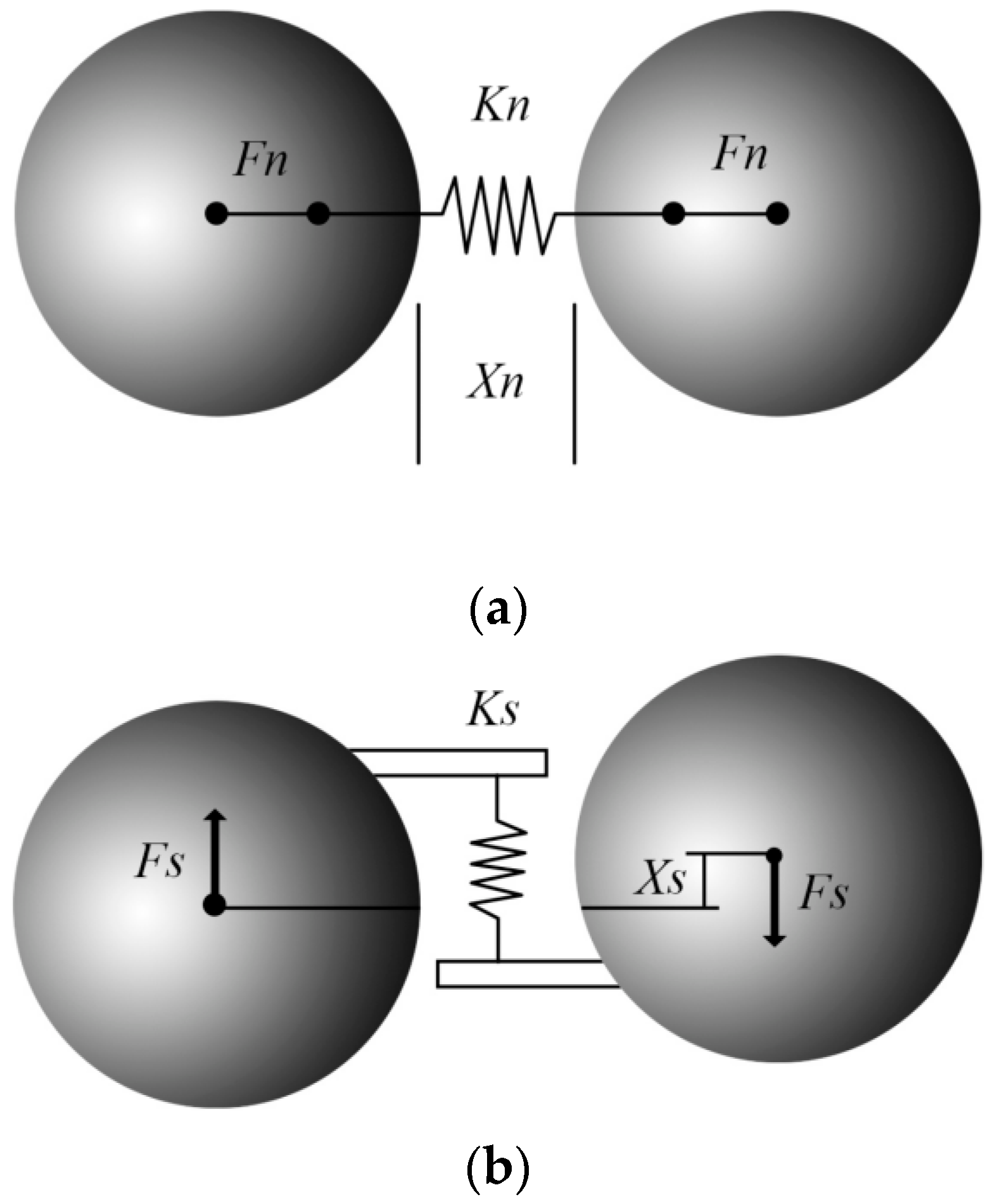
2. Selection of the Grain-Scale Contact Model

During numerical simulations by the discrete element method (DEM), a linear elastic contact model is adopted. In other words, a specimen is composed of a series of elastic elements (i.e., spheres) obeying Newton’s second law. Two elements are connected with each other by a breakable spring, and forces appear at the contact point between adjacent elements. The relationships between forces and displacements of the contact model in the normal and tangential directions are shown in Figure 1.
The normal force between elements, i.e., F n , is defined by
F n = K n X n
where Kn is the spring normal stiffness and Xn is the normal relative displacement. The tensile force exists when elements are connected to each other. When Xn exceeds the fracture displacement Xb, the connection is broken. Therefore, the maximum normal force between elements Fnmax is
F n m a x = K n X b
When the connection is broken, the tensile normal force between elements no longer exists. When the two elements return to the compressive contact state, the compressive normal force is rebuilt:
F n = K n X n ,   X n < 0
Additionally, the shear force Fs is also considered in the linear elastic contact model. When two elements contact and slide against each other, the sliding friction force opposite to the sliding direction is generated. The two elements are connected by a breakable spring in the tangent direction, and the tangential spring force Fs is defined by
F s = K s X s
where Ks is the shear stiffness and Xs is the tangential relative displacement. For a complete element connection, the maximum shear force Fsmax is determined by the Coulomb criterion:
F s m a x = F s 0 μ p F n
where Fs0 is the shear resistance in the tangential direction between elements, μ p is the friction coefficient between elements, and Fn is the normal force (compressive force is negative). When an external force exceeds the maximum shear force Fsmax, the tangent connection between elements is broken, and the shear resistance Fs0 disappears. In this case, the tangential force Fs is less than or equal to the maximum shear force Fsmax, which is defined by
F s m a x = μ p F n ,   when   the   connection   is   broken
In the case of connection fracture, elements slide when the external force exceeds the maximum shear force Fsmax. When the two elements are separated from each other ( X n > 0 ), the normal force and the tangential force between elements are zero.

3. Back Analysis of Grain-Scale Parameters

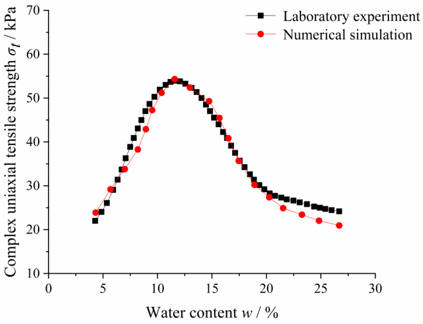
3.1. Determining Grain-Scale Parameters by Complex Uniaxial Tensile Test Simulation

MatDEM is a general discrete element software for geotechnical materials developed by Nanjing University. Based on the MATLAB calculation method, it adopts the innovative GPU matrix algorithm to realize the discrete element simulation of millions of particles. Its calculating number of units and efficiency are more than dozens of times that of other commercial software. On the basis of reaching the standard of hardware, it can complete the large-scale three-dimensional discrete element numerical simulation in a few hours. The software can realize the automatic modeling of discrete element materials and the calculation of energy conservation for discrete element systems. The software integrates pre-processing, calculation, post-processing, and powerful secondary development, provides a perfect function interface and efficient calculation engine, and completes complex multi-field coupling simulation through secondary development. MatDEM 1.32 version is adopted for this research.
For the convenience of discussion, hereafter the laboratory uniaxial tensile test is called a complex uniaxial tensile test. There are two groups of parameters in MatDEM, i.e., material parameters and grain-scale contact parameters. The material parameters include Young’s modulus ( E )/GPa, Poisson’s ratio ( ν ), tensile strength ( T u )/MPa, compressive strength ( C u )/MPa, and internal friction coefficient ( μ i ). The tensile strength T u refers to the tensile force when connections are broken, which is different from the complex uniaxial tensile strength. The grain-scale contact parameters include normal stiffness ( K n )/(MN/m), tangential stiffness ( K s )/(MN/m), failure displacement ( X b ), shear strength ( F s 0 )/N, and the friction coefficient ( μ p ). There is a clear relationship between the two groups of parameters in MatDEM.
The water content is a key influencing factor for the tensile strength of unsaturated soil. During a drying path, both the tensile stress and the tensile strength increase. When the tensile stress exceeds the tensile strength, the soil is damaged and the cracks occur. A relationship between tensile strength and water content could be obtained by comprehensive comparison between the results of complex uniaxial tensile tests and numerical simulation tests. Capillary cementation is a kind of apparent cohesion, which is the same as the cohesion contributing to the tensile strength T u . Therefore, a relationship between water content and microscopic tensile strength should be established according to simulations of triaxial tests for unsaturated soils.

3.2. Impact Analysis of Material Parameters on the Discrete Element Simulation

3.2.1. Creating a MatDEM Model for the Complex Uniaxial Tensile Test

A numerical model was generated according to the complex uniaxial tensile test of clay, and particles were also generated according to the particle size distribution and the maximum dry density of clay used in the laboratory test. It is difficult to generate a sample with a given void ratio due to particle equilibrium iterative cycles and compaction processes by the discrete element software. Only the average radius of particles (BallR) and the radius ratio of the maximum particle to the minimum particle (the distriRate parameter in the software represents the particle diameter dispersion coefficient, and the ratio of the maximum radius to the minimum radius is (1 + rate)2) are controlled. Considering that particle grading and void ratio affect the mechanical behavior of soil, the discrete element particle samples with specified particle grading and void ratio were generated by the Monte Carlo method.
The laboratory complex uniaxial tensile experimental apparatus consists of two symmetrical wedges (80 mm long and 10 mm thick). In order to make the specimen fail in the gap between the wedge-shaped molds, the neck width reduces from 40 to 20 mm in the middle part. One wedge is clamped to the press plate of the testing machine, and the other wedge is connected with the end crossbeam through the load sensor. The numerical wedges are generated by a filter and residual strength function, and the sample is generated inside the wedges. The specific wedges and numerical model are shown in Figure 2.

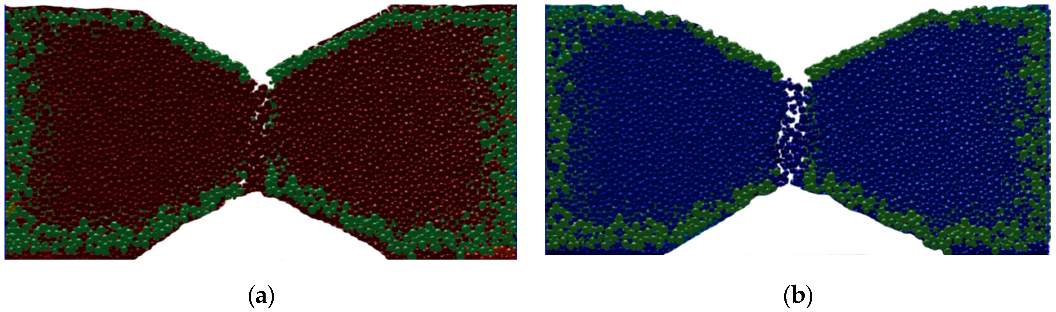
3.2.2. Loading Mode of the Numerical Model and the Calculation Rule of Tensile Strength

For a numerical tensile test, the loading plate moves outward with a constant displacement rate of 0.5 mm/min. During the test, the axial load and displacement are obtained continuously. The tensile stress σ t is
σ t = T / S
where T is the axial tensile load and S is the cross-sectional area (20 × 10 mm2). The peak tensile strength is the maximum tensile stress. The two wedges move in the opposite direction until a continuous failure surface is formed. The average value of contact stress along the tensile direction of two wedges at the failure state is taken as the tensile strength of the specimen. The tensile failure surface is shown in Figure 3.

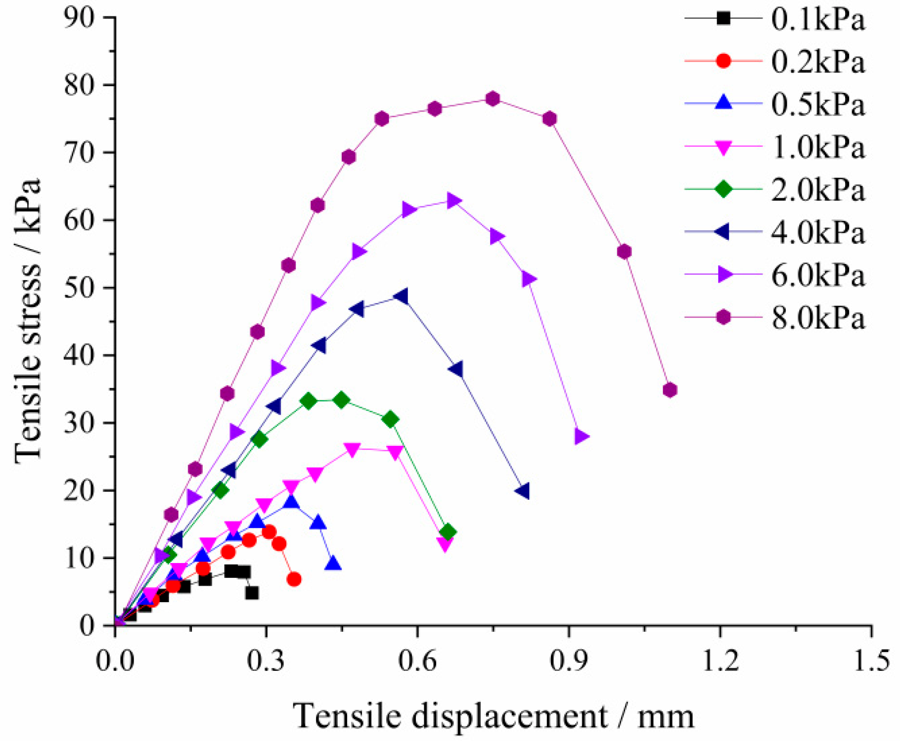
3.2.3. Influences of Material Parameters on the Complex Uniaxial Tensile Strength

Material parameters affect the properties of geotechnical materials by the discrete element method. Back analysis and a calibration method were used to determine the micro material parameters by complex uniaxial tensile strength.
  • Impact analysis of the tensile strength on the complex uniaxial tensile strength
If a tetrahedral element is used to study the mechanical properties of the model, the element is composed of four identical particles. As the force and displacement are very small, the analytical solution of tetrahedron deformation can be obtained. With the increasing of the tensile force (Fz) acting on the element, the relative displacement Xn1 of the top particles increases. When Xn1 > Xb, the connection between particles breaks. If Xn1 = Xb, the element tensile strength (Tu) is obtained:
T u = 6 2 K n K n + K s 3 K n + K s X b d 2
According to the tensile strength expression of the tetrahedral element composed of four elements, the tensile strength Tu is related to the spring normal stiffness K n , tangential stiffness K s , and the critical fracture displacement Xb. The values of the material parameters are shown in Table 1.
Through a large number of numerical tests with different tensile strengths Tu, it was found that the critical fracture displacements Xb obtained by automatic material training are different, and they also have a great influence on the tensile failure displacement of the complex uniaxial tensile simulation. As a result, the complex uniaxial tensile strength of the specimen increases with the increasing of tensile strength Tu. The simulation results are shown in Table 2 and Figure 4.
The mechanical properties of the model were also studied by the tetrahedral elements. The vertical compression and lateral expansion of an element are generated by tensile force Fz. When the relative displacement of the bottom particles exceeds the limit deformation (Xn2 > Xb), the horizontal connection breaks. Cu is the stress value in the vertical direction when the connection is broken horizontally, which is obtained by
C u = 6 2 K n K n + K s K n K s X b d 2
By fixing the tensile strength Tu, it is found that Cu affects the simulation results, and affects the spring normal and tangential stiffnesses.
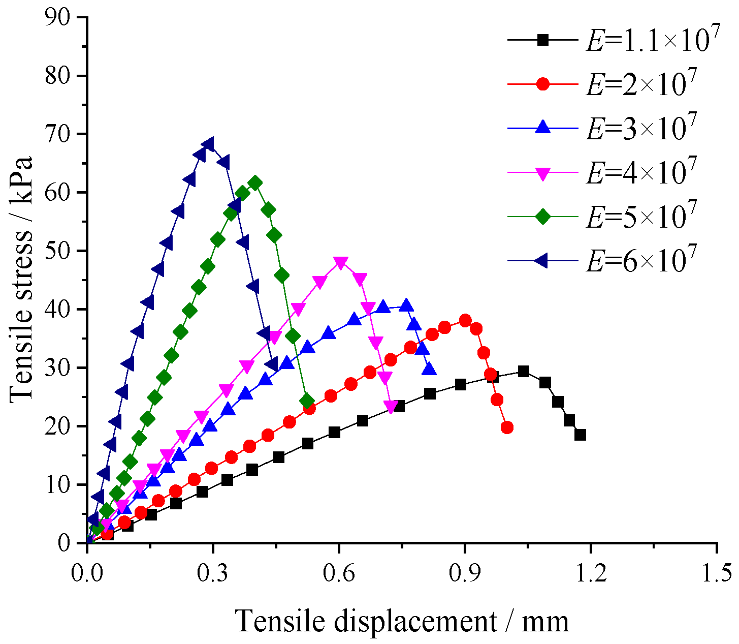
  • Impact analysis of Young’s modulus on the complex uniaxial tensile strength
The numerical simulation results by Boutt and Mcpherson [45] and Ergenzinger et al. [46] showed that the Young’s modulus increases with the increasing of particle stiffness. The complex uniaxial tensile numerical simulation was carried out by changing only the Young’s modulus (i.e., 1.1 × 10⁷, 2 × 10⁷, 3 × 10⁷, 4 × 10⁷, 5 × 10⁷, and 6 × 10⁷ Pa). Figure 5 shows the tensile stress–displacement curve with different Young’s moduli. It is shown that with the increasing of the Young’s modulus, the tensile displacement decreases.
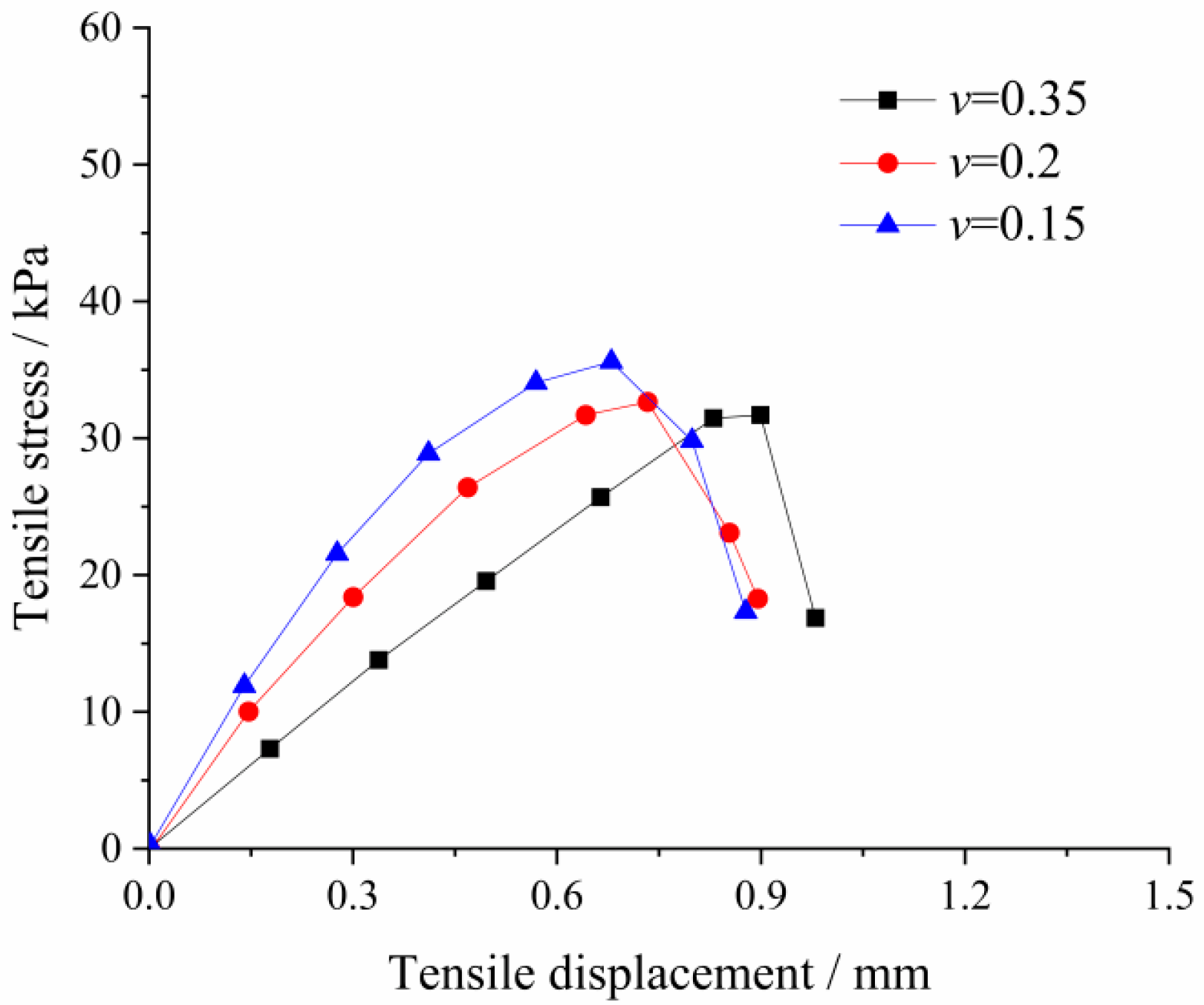
  • Impact analysis of Poisson’s ratio on the complex uniaxial tensile strength
Poisson’s ratio ν increases with the decreasing of the ratio of tangential stiffness to normal stiffness. In the linear elastic model, Poisson’s ratio ν can be calculated by
ν = ε x x ε z z = K n K s 5 K n + K s = 1 γ 5 + γ
where γ is the ratio of shear stiffness to normal stiffness. Equation (10) shows that ν decreases with the increasing of γ . When γ > 1, the negative Poisson’s ratio material can be obtained. The complex uniaxial tensile numerical simulation was carried out by changing only the Poisson’s ratio (i.e., 0.35, 0.2, and 0.15). Figure 6 shows the tensile stress–displacement curve with different Poisson’s ratios. The effect of Poisson’s ratio on the grain-scale parameters of particles is not significant.

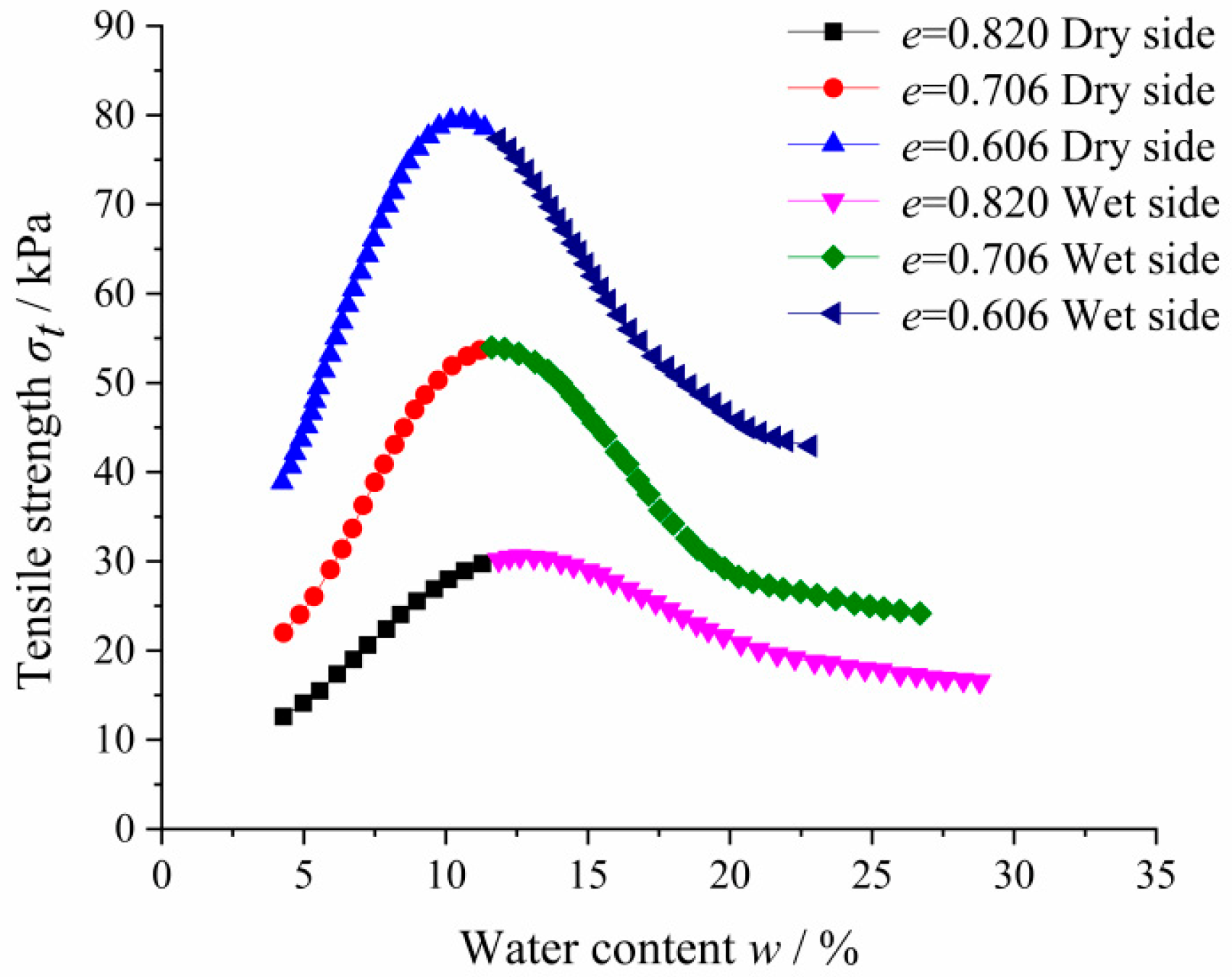
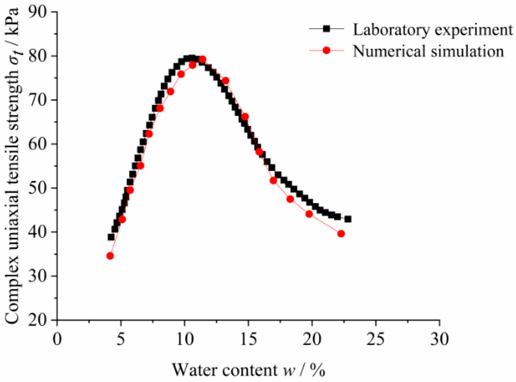
3.3. Relationship between Water Content and the Complex Uniaxial Tensile Strength of Unsaturated Clay

Thirty-two tensile strength tests by Tang et al. [10] were simulated. The clay, which was medium plastic clay, was from Nanjing, and the physical properties are shown in Table 3. The specific gravity was 2.73, the proportion of sand, silt, and clay was 2:76:22, and the elastic modulus was between 4 and 18 MPa. The initial dry densities were 1.5, 1.6, and 1.7 g/cm3, respectively, and the corresponding initial void ratios were 0.820, 0.706, and 0.606, respectively.
The complex uniaxial tensile test results are shown in Figure 7. For a given dry density, the uniaxial tensile strength σt significantly depends on the water content w. With the increasing of w, σt increases rapidly, and reaches the maximum value at the critical water content wc, corresponding to the peak value of uniaxial tensile strength. When the water content exceeds a certain value, the change of σt is very small with the further increasing of water content.
The experimental results with different initial void ratios were fitted by a second-order function.
(1)
Dry side (0 < w < 11.5%)
σ t = A d + B d w + C d w 2
where σ t is the uniaxial tensile strength, w is the water content, and Ad, Bd, and Cd are coefficients related to the initial void ratio under dry side. The values of Ad, Bd, and Cd for specimens with different initial void ratios are shown in Table 4.
(2)
Wet side (11.5% < w < 35%)
σ t = A w + B w w + C w w 2
where Aw, Bw, and Cw are coefficients under wet side. The values of Aw, Bw, and Cw for specimens with different initial void ratios are shown in Table 5.

3.4. Relation between the Tensile Strength Tu and Complex Uniaxial Tensile Strength σt

Based on the analysis results of the complex uniaxial tensile strength, it can be concluded that the influence of tensile strength Tu on the complex tensile strength σt is significant. Therefore, a series of numerical tests with different tensile strengths Tu was carried out. The numerical simulation of complex uniaxial tensile strength can be divided into three steps: (1) creating samples with the same particle size distribution as the laboratory experiment; (2) cutting the model, giving the material parameters, and balancing the model; and (3) applying the strain-controlled load by the user-defined function, and outputting the calculation results.
Based on the Monte Carlo method and the secondary development function of MatDEM, three groups of discrete element particle samples were generated with initial void ratios of 0.820, 0.706, and 0.606, respectively. The percentages of sand, silt, and clay for all of three groups were 2%, 76%, and 22%, respectively. If numerical particle sizes are the same as the real ones, millions of particles will be generated in this model. Therefore, considering the hardware limit, the radiuses of particles were uniformly reduced by a certain multiple. The average radius of the sample particles (BallR) was 5 × 10⁻⁴ m, the particle diameter dispersion coefficient (rate) was between 0 and 0.8, the minimum particle radius was 1.25 × 10⁻⁴ m, the maximum particle radius was 7.31 × 10⁻⁴ m, and the total number of particles was 65,139. The information of discrete element samples with specific initial void ratios is shown in Table 6.
Before numerical simulation, the particles of the model are piled up by gravity twice, so that all the particles are stable, and a pre-equilibrium model is obtained. Then, the model is cut and assigned material parameters. The values of the material parameters except for Tu are listed in Table 1.
After the model is established, the specimen is loaded by uniaxial tension. In order to obtain the completed stress–strain curve of the specimen, the loading speed is as slow as possible, and the change of stress is recorded after each displacement loading. It takes about 400 min for each specimen to complete the simulation. During loading, the sample is locked in the Y and Z directions. The model function d.mo.nfnx is used to monitor the change of contact force in the X direction. The complex uniaxial tensile simulation results of the samples with different tensile strengths Tu are shown in Table 7.
For the sample with an initial void ratio of 0.872, the numerical simulation results are fitted by a polynomial function, and the fitting relationship between the tensile strength Tu and complex uniaxial tensile strength σt is obtained by
σ t = 9.48315 + 1.72723 T u 0.02009 T u 2
The value range of Tu is 0 to 20 kPa, and the correction determination coefficient is 0.98722. Figure 8 is the simulation result with a tensile strength Tu of 4 kPa.

3.5. Relationship between MatDEM Material Parameters and the Water Content w of Unsaturated Clay

The complex uniaxial tensile strength expression of compacted clay with different dry densities and water contents is obtained according to the laboratory test results, and the relationship between the material parameter Tu and the complex uniaxial tensile strength with a given initial void ratio is obtained by numerical simulation. In the following, the relationship between the tensile strength Tu and water content w with a given initial void ratio is obtained through the intermediate value of complex uniaxial tensile strength.
According to the fitting results, when the initial void ratio e is 0.820, the fitting relationship between the material parameter tensile strength Tu and the complex uniaxial tensile strength σt is
σ t = 9.48315 + 1.72723 T u 0.02009 T u 2 ( 0 < T u < 20 kPa )
(1)
For the dry side (0 < w < 11.5%),
σ t = 3.14821 + 3.88897 w 0.08224 w 2
Substituting Equation (15) into Equation (14) obtains
T u = 1.7272 0.0066 w 2 0.3125 w + 3.9980 0.0402
(2)
For the wet side (11.5% < w < 35%),
σ t = 55.8452 2.40208 w + 0.03514 w 2
Substituting Equation (17) into Equation (14) obtains
T u = 1.7272 0.0028 w 2 + 0.1930 w 0.7423 ) 0.0402
Then, the material parameter Tu is obtained with different water contents. In order to verify the applicability of the fitting formula, the complex uniaxial tensile numerical simulation was carried out for unsaturated compacted clay with an initial void ratio of 0.706 and 0.606, respectively. According to the fitting results, numerical simulations for samples with different water contents were carried out, and the simulation results of the relationship between tensile strength and water content for the sample with an initial void ratio of 0.706 are shown in Figure 9. Figure 10 is the simulation result of the sample with an initial void ratio of 0.816 and water content of 20%.
For the sample with an initial void ratio of 0.606, the simulation results of the relationship between tensile strength and water content are shown in Figure 11. Figure 12 is the simulation result of the sample with an initial void ratio of 0.762 and water content of 15%. The fitting results show that the relationship between the material parameter tensile strength Tu and the water content w is suitable for simulating the tensile strength of unsaturated clay. According to this relationship, the discrete element numerical simulation of the triaxial tension–shear test for unsaturated soil will be carried out as the follows.

4. Simulation of Triaxial Tests for Unsaturated Soils under a Tension–Shear State

In this part, a group of triaxial test simulations for unsaturated soils under a tension–shear state is carried out. The stress path of triaxial test simulations is shown as follows: the sample is consolidated by confining pressure, then the axial stress gradually decreases. At the beginning of unloading, the specimen is elongated axially until the axial stress σ3 < 0. Finally, the specimen undergoes tensile failure. According to the results of numerical simulation, the variation of tensile–shear strength for unsaturated soil with confining pressures and water contents is revealed, and the triaxial tensile failure modes of unsaturated soil are analyzed.

4.1. Simulation Steps

The steps of the numerical test are introduced as follows. (1) The Monte Carlo method is used to generate discrete element particle samples close to the specified particle size gradation and void ratio. (2) According to the relationship between the water content w and tensile strength Tu, materials are trained automatically, and the trained materials are given to the model. (3) The stress is applied by the upper and lower pressure plates with the water confining pressure σ1. (4) The upper and lower pressure plates move to the opposite direction with a constant speed until the sample is damaged or a continuous failure surface is formed.

4.2. Simulation Results

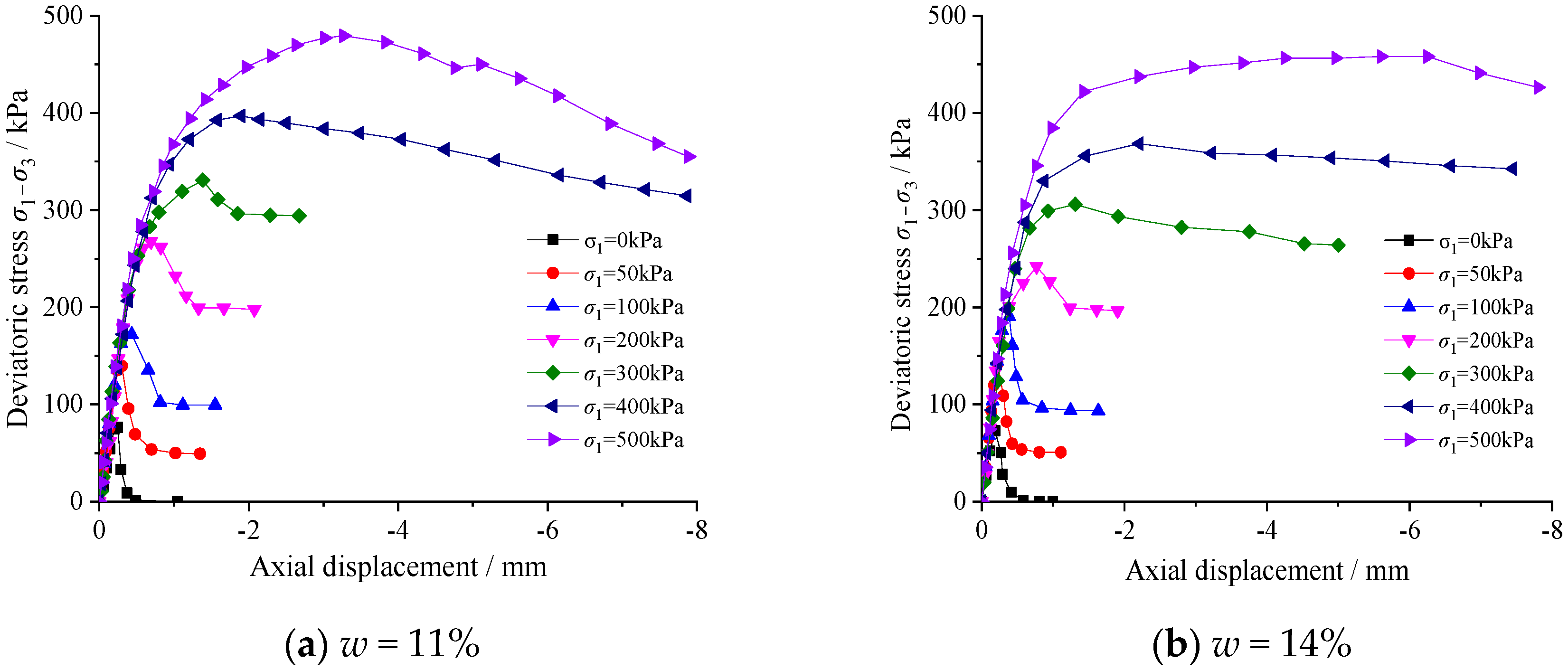
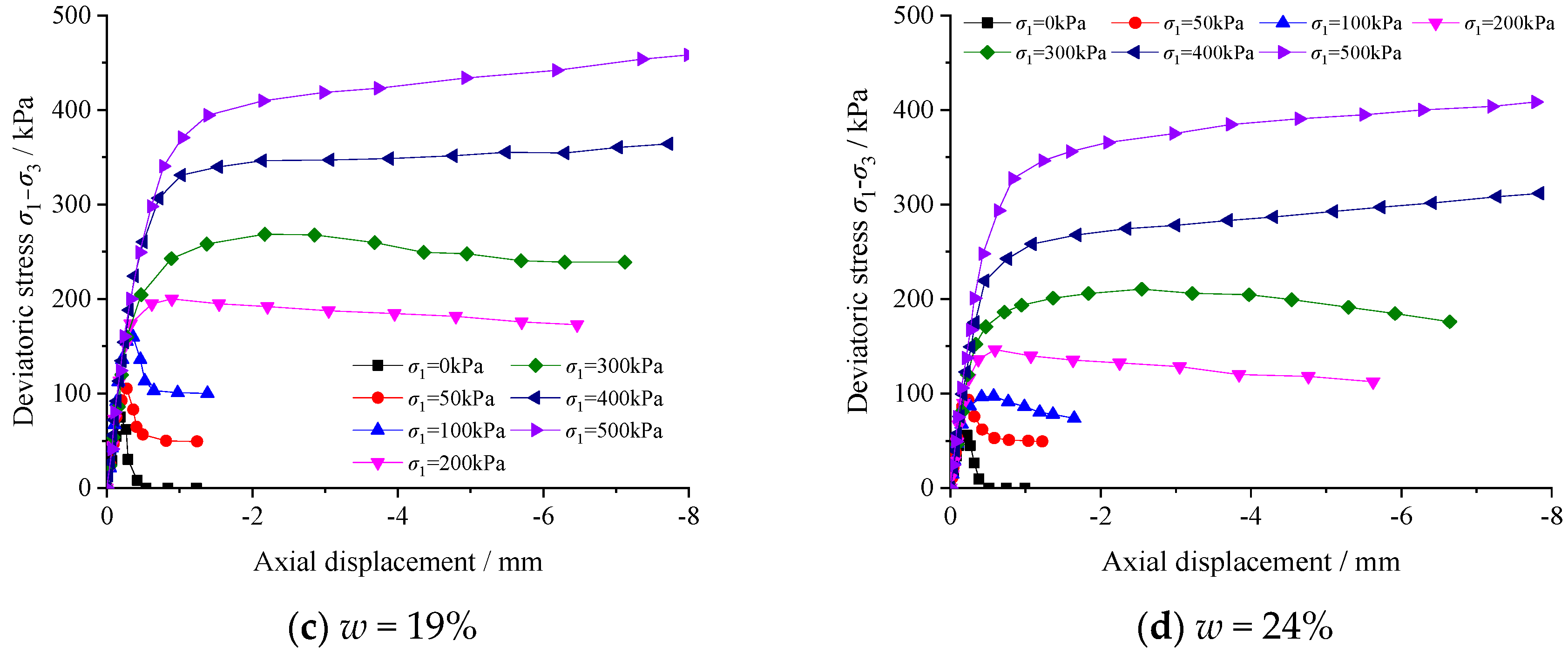
4.2.1. The Relationship between Deviatoric Stress and Axial Displacement

During the triaxial tensile simulation, the confining pressure is the large principal stress σ1, and the axial stress is the small principal stress σ3. The deviatoric stress is defined by σ1σ3. Figure 13 shows the discrete element numerical simulation results of samples with an initial void ratio of 0.872 with different confining pressures and water contents. For a given water content, the initial slopes of the deviatoric stress–axial displacement curve with different confining pressures are basically the same; however, the peak and residual strengths with different confining pressures are different. When the confining pressure is small (0 < σ1 < 200 kPa), the peak strength appears early, and the peak value is larger than the confining pressure σ1, which means that the axial stress σ3 reaches a tensile state. The deviatoric stress drops fast after the peak strength. Finally, the sample undergoes tensile failure, and the axial stress goes to 0. When the confining pressure is large (200 < σ1 < 500 kPa), the peak deviatoric stress increases with the increasing of confining pressure. The peak deviatoric stresses are basically less than or equal to the confining pressure σ1, which indicates that the axial stress σ3 is greater than 0. It should be noted that the water content affects the peak deviatoric stress and the hardening/softening characteristic. The strength increases with the decreasing of water content and the increasing of confining pressure. Moreover, the dilatancy phenomena is obvious for the samples with a low confining pressure and water content.

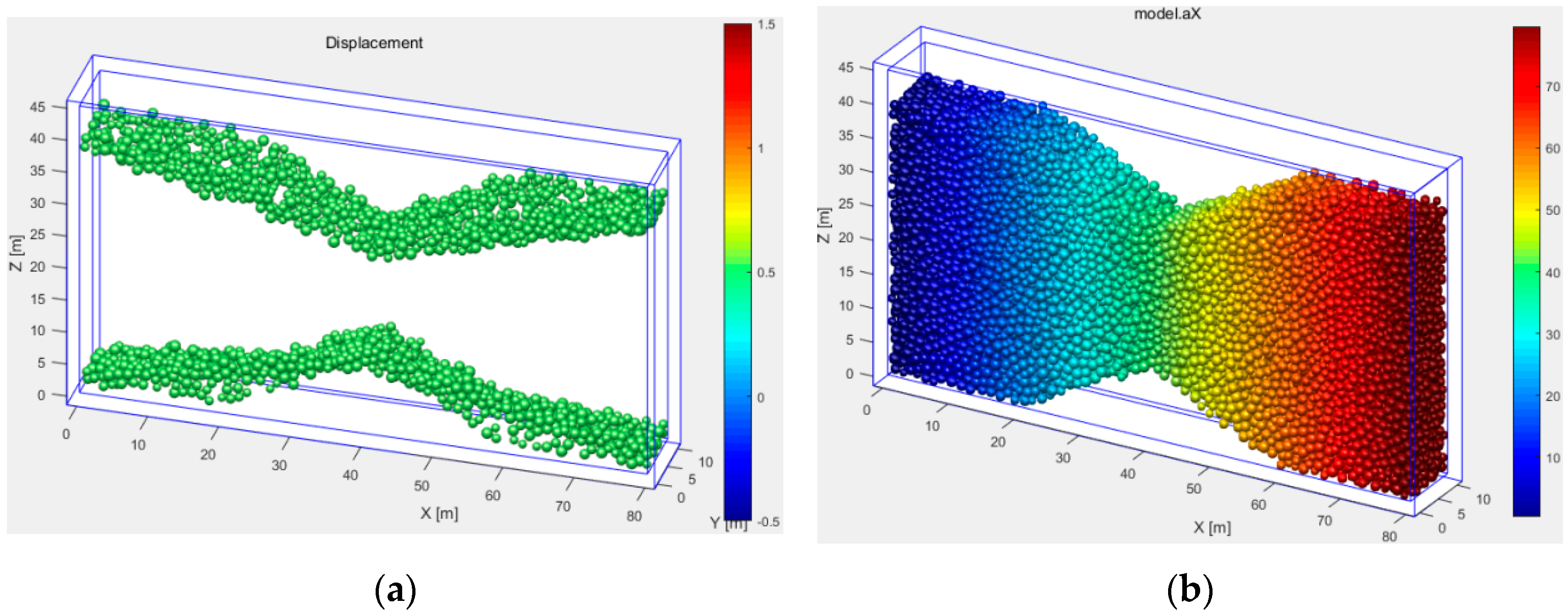
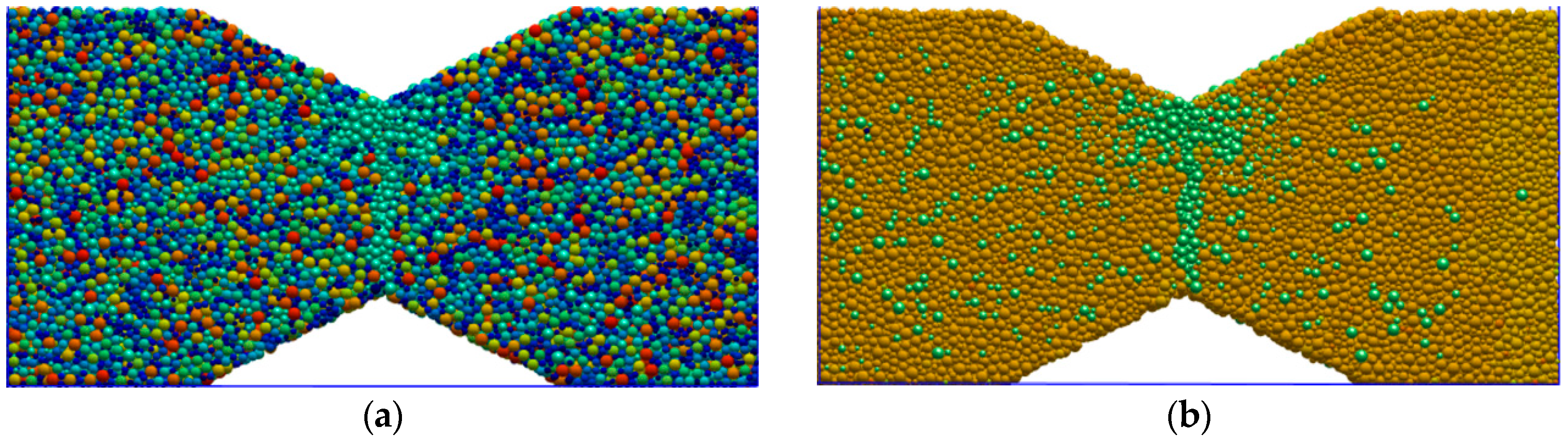
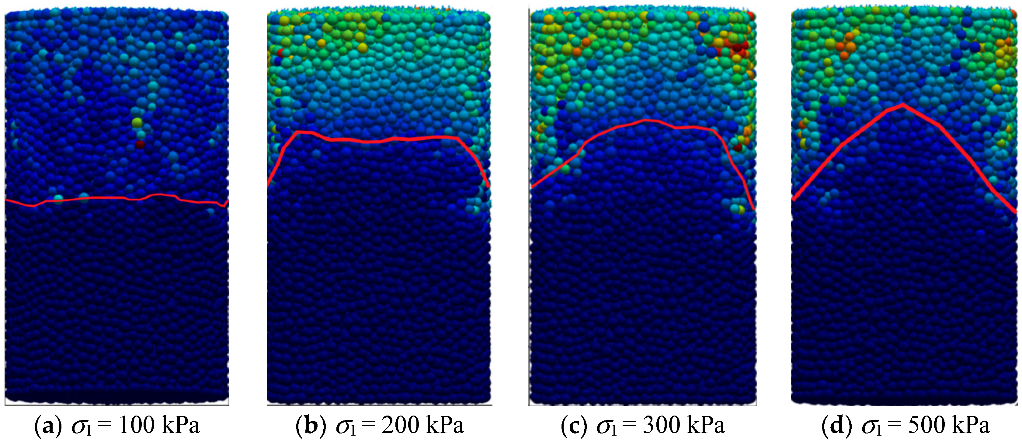
4.2.2. Displacement Field

Figure 14 shows the displacement field of specimens with different confining pressures. The particle color represents the displacement field. A brighter color means a larger displacement. The simulated results illustrate that the confining pressure affects the failure form of a specimen. When the confining pressure is small (σ1 = 100 kPa), the axial stress σ3 gradually changes from a compressive state to a tensile state. The fracture surface for tensile failure is basically horizontal.
When the confining pressure is in the middle range (σ1 = 200, 300 kPa), the failure modes of shear elongation and tensile fracture occur simultaneously. At the initial stage of loading, the four sides of the specimen remain straight. Then, a local inclined shear plane on the surrounding side of specimen appears when a threshold of tensile axial displacement is achieved. However, the shear plane does not develop to the interior of the specimen. Finally, the specimen fractures with the continuous increasing of the tensile axial displacement. According to the displacement field, the middle part of the fracture surface is basically horizontal, and local shear zones generate around the specimen.
When the confining pressure is large (σ1 = 400 kPa), the axial stress σ3 of specimen is always in the compressive state under the tensile loading path. With the increasing of tensile displacement, pure shear failure occurs; however, axial tensile stress does not appear. According to the displacement field, a shear band generates inside the specimen.

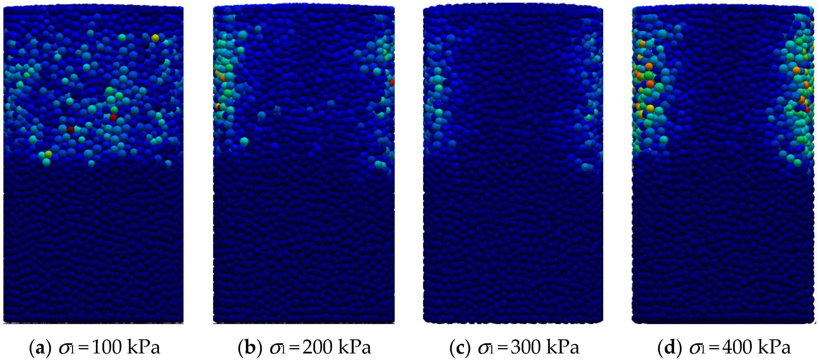
4.2.3. Heat and Energy Field

The simulation results of the heat field for samples with an 11% water content and different confining pressures are shown in Figure 15. The generated heat increases with the increasing of confining pressure. Based on the law of energy conservation, the total energy of the isolation system is constant. When the sample deforms under external forces, the increment of energy must be equal to the work done by the external force. For the same axial displacement, the mechanical energy of a sample with a high confining pressure is larger than that with a low confining pressure. The mechanical energy required for specimen failure increases with the increasing of confining pressure.

5. Conclusions

In this paper, a relationship between tensile strength and water content was obtained by comprehensive comparison between the results of complex uniaxial tensile tests and numerical simulation tests. Moreover, the discrete element simulation of triaxial tension–shear tests for unsaturated soils was carried out. The simulation results demonstrate the following:
  • The water content affects the peak deviatoric stress, dilatancy behavior, and failure mode.
  • The strength increases with the decreasing of water content and the increasing of confining pressure.
  • The dilatancy phenomena is obvious for the specimens with a low confining pressure range and water content.
  • The specimens undergo pure tensile failure under a small confining pressure condition, shear elongation and tensile failure under a middle confining pressure condition, and shear failure under a large confining pressure condition.

Author Contributions

Conceptualization, G.C.; Data curation, B.H., X.H. and C.Z.; Writing—review and editing, J.L. (Jian Li); Writing – original draft, S.L. and J.L. (Jiguang Li). All authors have read and agreed to the published version of the manuscript.

Funding

This research was funded by National Natural Science Foundation of China: (U2034204, 52078031); Beijing Natural Science Foundation: 8202038; Development Fund of Tunnel and Underground Engineering Research Center of Jiangsu Province: 2021-SDJJ-04; Fundamental Research Funds for the Central Universities: 2020JBM048; Fundamental Research Funds for the Central Universities: 2020CZ002; Regional Joint Fund Project of Basic and Applied Basic Research in Guangdong Province: 2019A1515111100; Young Creative Talents Program in Guangdong Province: 2019KQNCX170.

Institutional Review Board Statement

Not applicable.

Informed Consent Statement

Not applicable.

Data Availability Statement

The source of relevant data acquisition has been described in the text.

Conflicts of Interest

The authors declare no conflict of interest.

References

  1. Haefeli, R. Investigation and measurements of shear strength of saturated cohesive soil. Géotechnique 1951, 2, 186–208. [Google Scholar] [CrossRef]
  2. Parry, R.H.G. Triaxial compression and extension tests on remolded saturated clay. Géotechnique 1960, 10, 166–180. [Google Scholar] [CrossRef]
  3. Zhou, H.K. The mechanism of fracture of soil samples in triaxial tensile test. Chin. J. Geotech. Eng. 1984, 6, 12–23. (In Chinese) [Google Scholar]
  4. Yu, X.J.; Jiang, P. Experimental study on shocking crack of impervious soil in earth-rock dams. J. Hohai Univ. 1996, 24, 68–75. (In Chinese) [Google Scholar]
  5. Zhang, S.H.; Guo, M.X.; Xing, Y.C. Test technology on triaxial extension. J. Water Resour. Water Eng. 2001, 12, 24–27. (In Chinese) [Google Scholar] [CrossRef]
  6. Ibarra, S.Y.; McKyes, E.; Broughton, R.S. Measurement of tensile strength of unsaturated sandy loam soil. Soil Till. Res. 2005, 81, 15–23. [Google Scholar] [CrossRef]
  7. Lu, N.; Wu, B.; Tan, C.P. Tensile strength characteristics of unsaturated sands. J. Geotech. Geoenviron. 2007, 133, 144–154. [Google Scholar] [CrossRef]
  8. Zhu, C.H.; Liu, J.M.; Yan, B.W.; Ju, J.L. Experimental study on relationship between tensile and shear strength of unsaturation clay earth material. Chin. J. Rock Mech. Eng. 2008, 27, 3453–3458. (In Chinese) [Google Scholar] [CrossRef]
  9. Ran, L.Z.; Song, X.D.; Tang, C.S. Laboratorial investigation on tensile strength of expansive soil during drying. J. Eng. Geol. 2011, 19, 620–625. (In Chinese) [Google Scholar] [CrossRef]
  10. Tang, C.S.; Pei, X.J.; Wang, D.Y.; Shi, B.; Li, J. Tensile strength of compacted clayey soil. J. Geotech. Geoenviron. 2015, 141, 04014122. [Google Scholar] [CrossRef]
  11. Ji, E.; Chen, S.; Zhu, J.; Fu, Z. Experimental study on the tensile strength of gravelly soil with different gravel content. Geomech. Eng. 2019, 17, 271–278. [Google Scholar] [CrossRef]
  12. Li, H.D.; Tang, C.S.; Cheng, Q.; Li, S.J.; Gong, X.P.; Shi, B. Tensile strength of clayey soil and the strain analysis based on image processing techniques. Eng. Geol. 2019, 253, 137–148. [Google Scholar] [CrossRef]
  13. Alonso, E.E.; Gens, A.; Josa, A. A constitutive model for partially saturated soils. Géotechnique 1990, 40, 405–430. [Google Scholar] [CrossRef] [Green Version]
  14. Wheeler, S.J.; Sharma, R.S.; Buisson, M.S.R. Coupling of hydraulic hysteresis and stress-strain behaviour in unsaturated soils. Géotechnique 2003, 53, 41–54. [Google Scholar] [CrossRef]
  15. Gallipoli, D.; Gens, A.; Sharma, R.; Vaunat, J. An elasto-plastic model for unsaturated soil incorporating the effects of suction and degree of saturation on mechanical behaviour. Géotechnique 2003, 53, 123–135. [Google Scholar] [CrossRef]
  16. Li, X.S. Thermodynamics-based constitutive framework for unsaturated soils 2: A basic triaxial model. Géotechnique 2007, 57, 423–435. [Google Scholar] [CrossRef]
  17. Sun, D.A.; Sheng, D.C.; Xiang, L.; Sloan, S.W. Elastoplastic prediction of hydro-mechanical behaviour of unsaturated soils under undrained conditions. Comput. Geotech. 2008, 35, 845–852. [Google Scholar] [CrossRef]
  18. Charlier, R. Approche Unifiée de Quelques Problèmes non Linéaires de Mécanique des Milieux Continus par la Méthode des Éléments Finis. Ph.D. Thesis, Université de Liège, Liège, Belgium, 1987. [Google Scholar]
  19. Olivella, S.; Carrera, J.; Gens, A.; Alonso, E.E. Nonisothermal multiphase flow of brine and gas through saline media. Transp. Porous Med. 1994, 15, 271–293. [Google Scholar] [CrossRef]
  20. Chen, Y.; Zhou, C.; Jing, L. Modeling coupled THM processes of geological porous media with multiphase flow: Theory and validation against laboratory and field scale experiments. Comput. Geotech. 2009, 36, 1308–1329. [Google Scholar] [CrossRef]
  21. Wei, C.F. Static and Dynamic Behavior of Multiphase Porous Media: Governing Equations and Finite Element Implementation. Ph.D. Thesis, University of Oklahoma, Norman, OK, USA, 2001. [Google Scholar]
  22. Cundall, P.A. The Measurement and Analysis of Acceleration in Rock Slopes. Ph.D. Thesis, University of London, London, UK, 1971. [Google Scholar]
  23. Cundall, P.A.; Strack, O.D.L. A discrete numerical model for granular assemblies. Géotechnique 1979, 29, 47–65. [Google Scholar] [CrossRef]
  24. Fakhimi, A.; Carvalho, F.; Ishida, T.; Labuz, J.F. Simulation of failure around a circular opening in rock. Int. J. Rock Mech. Min. 2002, 39, 507–515. [Google Scholar] [CrossRef]
  25. Potyondy, D.O. A bonded-disk model for rock: Relating microproperties and macroproperties. In Proceedings of the Third International Conference on Discrete Element Methods, Santa Fe, NM, USA, 23–25 September 2002; pp. 340–345. [Google Scholar] [CrossRef]
  26. Potyondy, D.O.; Cundall, P.A. A bonded-particle model for rock. Int. J. Rock Mech. Min. 2004, 41, 1329–1364. [Google Scholar] [CrossRef]
  27. Backstrom, A.; Antikainen, J.; Backers, T.; Feng, X.T.; Jing, L.R.; Kobayashi, A.; Koyama, T.; Pan, P.Z.; Rinne, M.; Shen, B.T.; et al. Numerical modelling of uniaxial compressive failure of granite with and without saline porewater. Int. J. Rock Mech. Min. 2008, 45, 1126–1142. [Google Scholar] [CrossRef]
  28. Hsieh, Y.M.; Li, H.H.; Huang, T.H.; Jeng, F.S. Interpretations on how the macroscopic mechanical behavior of sandstone affected by microscopic properties—Revealed by bonded-particle model. Eng. Geol. 2008, 99, 1–10. [Google Scholar] [CrossRef]
  29. Sitharam, T.G.; Vinod, J.S.; Ravishankar, B.V. Post-liquefaction undrained monotonic behavior of sands: Experiments and DEM simulations. Géotechnique 2009, 59, 739–749. [Google Scholar] [CrossRef]
  30. Sadek, M.A.; Chen, Y. Simulating shear behavior of a sandy soil under different soil conditions. J. Terramechanics 2011, 48, 451–458. [Google Scholar] [CrossRef]
  31. Obermayr, M.; Dressler, K.; Vrettos, C.; Eberhard, P. A bonded-particle model for cemented sand. Comput. Geotech. 2013, 49, 299–313. [Google Scholar] [CrossRef]
  32. Xu, W.J.; Li, C.Q.; Zhang, H.Y. DEM analyses of the mechanical behavior of soil and soil-rock mixture via the 3D direct shear test. Geomech. Eng. 2015, 9, 815–827. [Google Scholar] [CrossRef]
  33. Jian, G.; Jun, L. Analysis of the thresholds of granular mixtures using the discrete element method. Geomech. Eng. 2017, 12, 639–655. [Google Scholar] [CrossRef]
  34. Zhu, X.; Liu, W.; Lv, Y. The investigation of rock cutting simulation based on discrete element method. Geomech. Eng. 2017, 13, 977–995. [Google Scholar] [CrossRef]
  35. Li, T.; Xiao, J. Discrete element simulation analysis of biaxial mechanical properties of concrete with large-size recycled aggregate. Sustainability 2021, 13, 7498. [Google Scholar] [CrossRef]
  36. Qi, Y.; Indraratna, B.; Ngo, T.; Ferreira, F.B. Advancements in geo-inclusions for ballasted track: Constitutive modelling and numerical analysis. Sustainability 2021, 13, 9048. [Google Scholar] [CrossRef]
  37. An, H.; Wu, S.; Liu, H.; Wang, X. Hybrid finite-discrete element modelling of various rock fracture modes during three conventional bending tests. Sustainability 2022, 14, 592. [Google Scholar] [CrossRef]
  38. Wang, Y.; Li, X.; Li, J.; Xu, J. Numerical simulation of impact rockburst of elliptical caverns with different axial ratios. Sustainability 2022, 14, 241. [Google Scholar] [CrossRef]
  39. Jiang, M.J.; Leroueil, S.; Konrad, J.M. Insight into shear strength functions of unsaturated granulates by DEM analyses. Comput. Geotech. 2004, 31, 473–489. [Google Scholar] [CrossRef]
  40. Trabelsi, H.; Jamei, M.; Zenzri, H.; Olivella, S. Crack patterns in clayey soils: Experiments and modeling. Int. J. Numer. Anal. Met. 2012, 36, 1410–1433. [Google Scholar] [CrossRef]
  41. Konrad, J.M.; Ayad, R. An idealized framework for the analysis of cohesive soils undergoing desiccation. Can. Geotech. J. 1997, 34, 477–488. [Google Scholar] [CrossRef]
  42. El Youssoufi, M.S.; Delenne, J.Y.; Radjai, F. Self-stresses and crack formation by particle swelling in cohesive granular media. Phys. Rev. E 2005, 71, 513–519. [Google Scholar] [CrossRef] [Green Version]
  43. Peron, H.; Delenne, J.Y.; Lalouia, L.; El Youssoufi, M.S. Discrete element modelling of drying shrinkage and cracking of soils. Comput. Geotech. 2009, 36, 61–69. [Google Scholar] [CrossRef]
  44. Sima, J.; Jiang, M.J.; Zhou, C.B. Modelling desiccation cracking in thin clay layer using three-dimensional discrete element method. In Proceedings of the 7th International Conference on the Micromechanics of Granular Media (Powders and Grains 2013), Sydney, Australia, 8–12 July 2013; pp. 245–248. [Google Scholar] [CrossRef] [Green Version]
  45. Boutt, D.F.; Mcpherson, B.J.O.L. Simulation of sedimentary rock deformation: Lab-scale model calibration and parameterization. Geophys. Res. Lett. 2002, 29, 13-1–13-4. [Google Scholar] [CrossRef] [Green Version]
  46. Ergenzinger, C.; Seifried, R.; Eberhard, P. A discrete element model to describe failure of strong rock in uniaxial compression. Granul. Matter. 2011, 13, 341–364. [Google Scholar] [CrossRef]
Figure 1. Force–displacement relationships of contact model: (a) normal direction and (b) tangential direction.
Sustainability 14 09122 g001
Figure 2. Schematic diagram of simulation model: (a) numerical wedges and (b) complex uniaxial tensile numerical model.
Sustainability 14 09122 g002
Figure 3. The simulation results of complex uniaxial tensile test at failure state: (a) stress field and (b) interparticle contact force chain.
Sustainability 14 09122 g003
Figure 4. Impact analysis of tensile strength on complex uniaxial tensile strength.
Sustainability 14 09122 g004
Figure 5. Impact analysis of Young’s modulus on complex uniaxial tensile strength.
Sustainability 14 09122 g005
Figure 6. Impact analysis of Poisson’s ratio on complex uniaxial tensile strength.
Sustainability 14 09122 g006
Figure 7. Tensile strength characteristic curves.
Sustainability 14 09122 g007
Figure 8. Simulated result (Tu = 4 kPa): (a) force field and (b) X-displacement field.
Sustainability 14 09122 g008
Figure 9. Relationship between tensile strength and water content for the sample with initial void ratio of 0.706.
Sustainability 14 09122 g009
Figure 10. Simulated result of sample with initial void ratio of 0.816 and water content of 20%: (a) stress field and (b) displacement field.
Sustainability 14 09122 g010
Figure 11. Relationship between tensile strength and water content for the sample with initial void ratio of 0.606.
Sustainability 14 09122 g011
Figure 12. Simulated result of “X-displacement” for sample with initial void ratio of 0.762 and water content of 15%.
Sustainability 14 09122 g012
Figure 13. Simulation results with different confining pressures and water contents.
Sustainability 14 09122 g013aSustainability 14 09122 g013b
Figure 14. Simulation results of displacement field with different confining pressures.
Sustainability 14 09122 g014
Figure 15. Simulation results of heat field with different confining pressures.
Sustainability 14 09122 g015
Table 1. Material parameters.
Average Particle Radius
rave/m
Particle Diameter Dispersion Coefficient RateSpecific Gravity
Gs
Young’s Modulus
E/MPa
Poisson’s Ratio
ν
Compressive Strength
Cu/kPa
Internal Friction Coefficient of Material
μi
0.0020.62.73200.3200.4
Table 2. Complex uniaxial tensile strength with different tensile strengths Tu.
VariableValue
Tensile strength Tu/kPa0.10.20.512468
Tensile failure displacement /mm0.2300.3060.3490.4700.4490.5700.6690.749
Complex uniaxial tensile strength /kPa8.08113.87218.18226.26333.40148.75462.89677.979
Table 3. Physical properties of clay.
Soil PropertiesSpecific GravityConsistency LimitUSCS ClassificationCompaction CharacteristicsParticle Size Analysis
Liquid Limit (%)Plastic Limit (%)Plasticity Index
(%)
Optimum Water Content (%)Maximum Dry Density (g/cm3)Sand (%)Silt (%)Clay (%)
Value2.73372017CL16.51.727622
Table 4. Fitting parameters for dry side.
Initial Void Ratio eAdBdCdDetermination Factor
0.820−3.148213.88897−0.082240.99546
0.706−12.373978.52281−0.222180.98924
0.606−29.4086118.88517−0.810920.99389
Table 5. Fitting parameters for wet side.
Initial Void Ratio eAwBwCwDetermination Factor
0.82055.8452−2.402080.035140.9753
0.706132.56575−8.207540.155160.9791
0.606184.43806−11.74870.242320.99729
Table 6. Numerical samples with specific initial void ratios.
Initial Dry Density g/cm3Particle Size Analysis
%
Initial Void Ratio eTotal Number of Particles
1.5Laboratory testSand/Silt/Clay2/76/220.82065,139
Numerical testSand/Silt/Clay1.3/74/24.70.872
1.6Laboratory testSand/Silt/Clay2/76/220.70665,338
Numerical testSand/Silt/Clay1.8/78/20.20.816
1.7Laboratory testSand/Silt/Clay2/76/220.60666,327
Numerical testSand/Silt/Clay2.2/76/21.80.762
Table 7. Complex uniaxial tensile simulation results.
Initial Void Ratio for Laboratory Test
e0
Initial Void Ratio for Numerical Test
e0
Total Number of ParticlesTensile Strength Tu/kPaComplex Uniaxial Tensile Strength
/kPa
Complex Uniaxial Tensile Failure Displacement /mm
0.8200.87265,1390.510.120.12
112.230.15
213.450.25
314.110.34
415.450.38
516.890.40
617.980.42
719.560.45
822.460.48
924.560.51
1025.790.58
1126.890.67
1227.360.75
1328.450.80
1429.350.86
1530.150.89
1632.120.95
Publisher’s Note: MDPI stays neutral with regard to jurisdictional claims in published maps and institutional affiliations.

