Abstract
Energy efficiency and energy intensity are gradually gaining attention, and it is now an important proposition to reconcile financial development, green finance, and regional energy intensity. Using Chinese mainland provincial panel data (except Tibet) from 2007 to 2019, this paper applied the spatial econometric model and the panel threshold model to investigate the effects of financial development and green finance on regional energy intensity. The paper discovered that financial development raises regional energy intensity, while green finance reduces it. Based on the panel threshold perspective, in different stages of green finance development, the effect of financial development on regional energy intensity presents an inverted U-shaped effect that first promotes and then inhibits. Meanwhile, green finance has a significant positive spatial transmission effect on regional energy intensity. Based on the spatial weight matrix reflecting regional economic relations, the increase in energy intensity has a significant negative spatial autoregressive effect on itself, and the spatial spillover effect of financial development is negligible.
1. Introduction
Energy and climate challenges have garnered consistent attention in recent years [1], and how to achieve high-quality economic development has become a key concept [2]. China is the world’s largest consumer of energy, and the Chinese government has set the goal of “carbon peaking” by 2030 and achieving “carbon neutrality” by 2060 in response to the deterioration of China’s climate and energy security issues [3]. The accomplishment of this target is dependent on China’s ability to enhance energy use efficiency. However, due to China’s inherent scarcity of energy and the deterioration of its environmental carrying capacity, the model of high economic growth exchanged for high energy consumption after the reform and opening up can no longer be sustained, and various measures must be implemented to improve the efficiency of energy use in the development process [4]. Throughout this process, the regional energy intensity might be an essential metric used by energy economists to quantify regional energy usage efficiency (that is, the ratio of energy consumption to output in a country or region). This is because lowering energy intensity implies not only a rise in the provision of public goods but also an improvement in regional productivity levels, which may create more output while using less energy [5,6,7].
With the rapid development of finance, in addition to its direct effect on economic development, its role in China’s environmental benefits and energy-saving development has also attracted wide public attention in China. Financial development can promote regional and corporate technological innovation [8,9] and increase the output value per unit of energy consumption, which in turn has a suppressive effect on regional energy intensity. Further, financial development creates some problems: it can provide more investment and financing channels for society, thus creating an aggregate investment effect. However, as traditional high energy-consuming industries are obtaining more funds for expansion through financial instruments, the energy use efficiency would be inhibited [10]. In addition, compared to the technically complex, long-cycle, low short-term return high-tech, and clean-tech industries, the financial market players are more willing to invest financial resources into traditional industries with relatively mature technologies. Furthermore, in the current Chinese context, the financial market is monopolized by commercial banks and is subject to excessive government intervention [11,12]. Thus, it is difficult to achieve efficient resource allocation. More seriously, local governments and officials are more willing to engage in short-term economic behavior due to the regional GDP (Gross Domestic Product) competition tournaments. Therefore, they are more likely to tilt policies toward traditional high-consuming industries and not favor high-tech industries with low reliance on energy. The monopolization of financial markets and excessive government intervention in financial markets would unavoidably result in a decrease in regional energy usage efficiency and an increase in regional energy intensity.
As China’s economic development enters a new normal, green finance gradually shows a trend of dominating the financial market and gradually has an important impact on the external effects of the development of the financial market on regional energy intensity [13]. As an economic activity to deal with climate change and prevent further deterioration of the environment, green finance has become the main support for the development of the green economy and a new engine for adjusting the industrial structure and promoting high-quality economic development. In 2016, the People’s Bank of China, together with seven ministries and commissions, issued the “Guiding Opinions on Building a Green Financial System”, which defined green finance as an economic activity that supports environmental improvement, addressing climate change and resource conservation and efficient use, that is, environmental protection, energy conservation, clean energy, green transportation, green building and other fields of project financing, project operation, risk management, and other financial services provided. In order to encourage banking financial institutions to expand their green finance business, in May 2021, the People’s Bank of China issued the “Green Finance Evaluation Plan for Banking Financial Institutions” to provide normative guidelines for coordinating the green finance evaluation of banking financial institutions. It is generally believed that green finance can optimize resource allocation, promote ecological and resource protection, promote industrial structure adjustment and economic transformation and upgrading, and then improve the level of energy utilization in the region. However, at the same time, China’s green finance development process is still in its infancy. There are problems such as an imbalance of incentive and restraint mechanisms for investment and financing entities, a lack of mature institutional investors, and difficulty in the operation and supervision of green projects. There are also ethical issues such as “dyeing green” and “washing green” in the market. There is risky behavior, and investors are mainly concerned about the economic benefits of investment, but not enough attention has been paid to the disclosure of important information such as social benefits, end use of raised funds, and the degree of greening of the project, which will result in poor financial entities after “greening” to drive out benign financial entities, resulting in a negative impact on regional energy utilization.
In conclusion, financial development and green finance have a huge impact on regional energy intensity, and the advantages and shortcomings themselves will also have completely different effects on regional energy intensity. Since the three economic variables have not yet been placed in a unified research framework for analysis, a complete theoretical mechanism has not yet been formed. To this end, this paper will focus on the three economic variables of financial development, green finance, and regional energy intensity, using the panel data of 30 provinces in mainland China (excluding Tibet) from 2007 to 2019. First, this paper investigates the separate effects of green finance, financial development, and their spatial effects on regional energy intensity by constructing a spatial econometric model. Then, this paper investigates the joint influence mechanism of financial development and green finance on regional energy intensity by constructing a panel threshold model.
2. Literature Review
2.1. Literature Review of Studies Related to Financial Development and Regional Energy Intensity
There is a dearth of international studies on how finance affects energy intensity and energy efficiency, and the majority of current research focuses on how the financial sector affects regional energy use. Islam et al. [14] included financial development with the GDP and population in a unified research framework to explore the interaction between the three and regional energy consumption; Mahalik et al. [15] demonstrated the importance of financial development in boosting national demand for energy through a study of panel data in Saudi Arabia. At the same time, two perspectives on the relationship between regional energy use and financial development have steadily arisen in academia. Starting from the “environment–economy–energy” analytical paradigm, some academics contend that financial development has increased society’s energy consumption while fostering economic expansion and, in general, decreased the efficiency of energy usage [16,17]. Another group of academics states that financial development can help to advance social and technological advancement, environmental awareness, and industrial structure optimization and upgrading, all of which can help to lower energy use and boost energy efficiency [18,19].
In the Chinese context, Sun Puyang et al. [20] verified that financial development can promote the upgrading of the energy structure by changing the demand for and consumption of energy through cross-country empirical analysis. However, the majority of scholars pointed out that the impact of financial development on regional energy consumption in China shows an inverted U-shape, i.e., it can promote energy consumption in the short term, but based on the long term, financial development can significantly inhibit regional energy consumption [21,22].
Based on the aforementioned review of the literature, it can be concluded that current research focuses on the effect of financial development on energy consumption. However, there are few studies on the relationship between financial development and energy intensity, and therefore more research is necessary in this area.
2.2. Literature Review of Studies Related to Green Finance and Regional Energy Intensity
The academics have not yet developed a consensus definition of green finance. According to the more common perspective, green finance can encourage societal environmental protection and direct participants in the financial markets to make investments that are environmentally friendly [23]. However, Chinese scholars, who tend to focus on the domestic situation and the development of China’s ecological civilization, emphasize the impacts that environmentally friendly credit, insurance, and other financial derivatives have on local energy use efficiency and eco-efficiency [24].
International research on the interaction between green finance and regional energy intensity is scarce and tends to focus on the micro (firms, individuals) and meso (industries) levels. Most scholars outside China have tested the Porter hypothesis to show that the development of green finance can indirectly improve energy use and curb energy intensity by increasing the level of technological innovation in firms and industries [25]. In the Chinese context, the impact of green finance on energy intensity is controversial. Some scholars believe that green finance can promote the technological progress of enterprises by regulating innovation awareness, innovation structure, and innovation mechanisms, thus enhancing the development of regional green industries and indirectly reducing energy intensity [26], while green finance can prompt enterprises’ technological innovation to favor environmentally friendly technologies such as high-tech, environmental protection, and clean technologies, further reducing energy intensity [27]. Another group of academics contends that because China’s green finance industry was slow to emerge and has grown significantly, costs for businesses have gone up, reducing their liquidity and stifling technological innovation. Furthermore, the current green finance system lacks a legally binding incentive mechanism, and green financial instruments frequently do not adequately support industrial technological innovation, leading to a misallocation of resources. Additionally, there is widespread “greenwashing” on the market, which has a detrimental effect on energy efficiency [28].
According to the aforementioned literature, there are not many studies on green finance and regional energy intensity. Additionally, research on the macro level (national and regional) is lacking, with the majority of current studies concentrating on the micro and meso levels. Meanwhile, the current research mainly discusses the relationship between green finance and energy intensity indirectly through the influence mechanism of green finance with respect to industrial structure and technological innovation, with a lack of research on the direct relationship between the two. Furthermore, there is still debate on the ways that green finance affects energy intensity in the Chinese context, and this paper tends to fill in those research gaps.
Considering that there is a direct or indirect relationship between financial sector development and industrial layout as well as economic orientation, it is necessary to include green finance, financial development, and regional energy intensity in the same research framework. Analysis of the effects of financial development and green finance on regional energy intensity and a discussion of the combined effects of these two factors on regional energy intensity are both indispensable. In addition, given that this paper attempts to study the mechanism in a macro-regional context, it is also necessary to consider the spatial spillover effects of individual economic variables to improve the accuracy of the analysis on the one hand and to seek the spatial transmission mechanism of economic variables on the other.
3. Theoretical Mechanism
3.1. Financial Development and Energy Intensity: “Preference Mismatches” and “Capital Market Distortions”
Although financial development can assist firms in mitigating information asymmetries and restructuring industries [29,30,31], such technological progress is biased toward shorter-cycle and less risky traditional energy-intensive industries rather than high-tech and clean production technologies [32,33,34]. The misallocation of financial resources caused by this preference also causes financial resources and funds to be more inclined to support traditional enterprises with high short-term returns and high energy waste, which increases the energy consumption per unit of output. Furthermore, under the current situation of China’s financial development, state-owned commercial banks have an oligopolistic tendency and form collusion among industries [35,36], which hinders the improvement of the utilization efficiency of financial resources and causes capital mismatch to a certain extent. In addition, the long-term absolute high market share of state-owned commercial banks in the financial market does not come from market choice but depends more on the will of the government [37]. The government’s distortion of the financial market is behind this oligopoly. Under the current tournament-style official promotion system in China, local governments and officials in charge, out of their own promotion needs, will tend to focus more on mature technologies and short cycles in terms of policies and resources, forming a “government–enterprise conspiracy” [38] with such enterprises to obtain maximum economic growth benefits. Relying on path dependence, traditional industries occupy the market share and squeeze out the living space of high-tech industries and green technology enterprises, resulting in capital market distortion and resource misallocation, reducing energy utilization efficiency.
The following hypothesis is derived from the analysis of the above mechanism:
Hypothesis 1 (H1).
Regional energy intensity increases considerably as a result of financial development.
3.2. Green Finance and Regional Energy Intensity: Mitigation Effects
Green finance is emerging as a critical strategy for reducing regional energy intensity in the context of “peak carbon” and “carbon neutral” ambitions. Green finance has the potential to both promote and inhibit regional energy efficiency at multiple levels.
At the micro-level, green finance can provide exogenous financial capital assistance for environmentally friendly firms such as high-tech enterprises and green technology enterprises. At the same time, as the green finance industry continues to grow, green finance provides investors with more investment options and investment tools for environmentally friendly investments, and the green competition signal conveyed by China’s green finance industry motivates companies to launch a new round of green competition. This is also conducive to improving regional environmental efficiency and energy use [39].
Based on the mesoscopic level, in the long run, the development of green finance and system construction can significantly promote the upgrading of the industrial structure and can promote industry innovation. The mechanism is that the capital allocation function of green finance can allocate more to environmentally friendly and energy-saving industries’ financial resources and then guide the optimization and upgrading of the industrial structure, comprehensively restraining the regional energy intensity [40,41].
On a macro level, green financing can also provide positive externalities regarding regional environmental benefits and energy use levels. Firstly, green finance can guide policies to accurately predict regional technological gains and ensure the effectiveness of environmental policies [42]. Secondly, green finance can force the government to improve the intensity of environmental regulations and develop environmentally friendly policies to implement supply-side structural reform in China. At the same time, the development of green finance implies financial innovation that seeks the path of environmental protection, and the development of green finance has become an unavoidable demand for the financial industry’s innovation and sustainable development [43,44]. This innovation is conducive to alleviating the oligopoly of the financial market, breaking the trap of path dependence, and leading the industrial structure and corporate investment and financing behavioral decisions to an environmentally friendly direction, which in turn curbs regional energy intensity across the board.
The following hypothesis is derived from the analysis of the above mechanism:
Hypothesis 2 (H2).
Green finance development has considerable potential to reduce regional energy intensity.
3.3. Financial Development, Green Finance, and Regional Energy Intensity: “Moderating Effects” and “Inverted U-Shaped Effects”
Green finance not only has positive externalities on regional energy consumption, it also functions as a positive factor in the financial industry and can achieve the regulation of negative externalities generated throughout the financial development process. Green finance tools and product innovation can change the way people think about financial market investment and financing, particularly in light of the capital market distortion caused by capital subjects’ preference to invest in traditional high-energy-consuming industries in pursuit of short-term capital returns. Green finance, through new financial innovation tools and investment and financing channels, can also effectively break this “preference mismatch,” and steer financial development in an environmentally friendly direction [45,46,47] so that it inhibits energy intensity in reverse.
Due to the late start, small scale, and low level of development of green finance in developing countries represented by China, there are problems such as single financial instruments and lagging financial innovation at the early stage of development [48,49]. In addition, the green finance market and some enterprises in the Chinese context still have phenomena such as “greenwashing” and “green bleaching” [50]. Therefore, in the early stage of green finance development, it is not yet possible to effectively regulate the negative impacts of the financial development process. As the scale of green finance expands and the green finance market regulation system and regulatory measures improve, the financial industry’s negative influence on regional environmental benefits and energy use efficiency is reduced. When green finance develops to a certain scale, the green finance industry will occupy a dominant position in the financial industry, continue to exert the “driver effect” of high-quality financial resources formed by the scale effect, and drive financial resources to agglomerate in a large number of environmentally friendly and energy-saving industries, so that the financial development reversely restrains the regional energy intensity. Accordingly, under green finance regulation, financial development has a non-linear “inverted U-shaped” impact on regional energy intensity, which is first boosted and subsequently inhibited.
The following hypothesis is derived from the analysis of the above mechanism:
Hypothesis 3 (H3).
When the level of green finance is low, the financial development will increase the regional energy intensity, and when green financial development reaches a certain level, the negative effect of financial development will be corrected.
3.4. Spatial Effect: “Polarization Effect” and “Bottom-To-Bottom Extrusion”
Economic and financial interactions between regions have become more frequent as China’s market economy has been developing, particularly in recent years with the gradual formation of a unified cross-regional financial market. This has allowed financial resources and other economic factors to circulate between regions, which has inevitably led to economic benefit spillover. According to the research framework, green finance can help enterprises and regions achieve the upgrading of green technologies through R&D subsidies, environmental regulation, and risk reduction in innovation [51]. However, because the development of high-tech and green technologies is characterized by their long cycle time and technical complexity while traditional finance has obvious path preference, the development of high-tech and green technologies can rely strongly only on the support of green finance [52]. Owing to the relative scarcity of green financial resources, it is easy for regions to compete for green financial resources, forming a spatial “siphon effect” and “polarization effect”. [53,54,55]. Meanwhile, due to the late start and low overall development level and efficiency of green finance in China, there is often a shortage of financial resources [56]. Moreover, at this stage, green finance might inhibit itself from forming a scale effect due to technical complexity, inadequate information disclosure, and “floating green” [57,58]; then, the positive externalities generated by green finance in the region’s energy intensity will not be large enough for it to spread to other regions, and it will not be able to form a significant “diffusion effect” and “trickle-down effect” that will benefit other regions’ environmental benefits and energy use efficiency. In addition, in the context of the Chinese competition of regional governments, local governments compete around economic growth. Usually, this competition is characterized by a “zero-sum game” situation, not by Pareto improvements.
In terms of regional economic and social development levels, regions with low energy intensity are economically developed, possess better technical conditions, and have higher green production efficiency. These conditions enables those regions to have a siphoning and magnetizing effect on other regions’ talents, capital, and technology, which are conducive to improving energy efficiency and mitigating energy intensity. Similarly, the business environment, technical levels, and policy conditions of regions with higher energy intensity are not conducive to the activities of green industries and their related factors, forming a siphoning and agglomeration effect on ecologically destructive and energy-wasting industries [59]. At the same time, as a developing country with relatively scarce resources for development and innovation, the “zero-sum game” and disorderly competition between regions in China have exacerbated the widening gap in energy intensity levels between regions [60]. Therefore, as the competition for green financial resources and innovation resources gradually heats up, this competition has a negative impact on regional innovation, environmental efficiency, and the industrial structure [61]. Based on the above analysis, the spatial effect of green finance in one region will hinder the process of reducing energy intensity in other regions. That is, while the development of green finance in a province can effectively suppress regional energy intensity, it also has significant negative spatial externalities. Further, the increase in regional energy intensity is frequently accompanied by ineffective resource allocation, unreasonable industrial structure, and declining regional innovation level in that region. Therefore, by squeezing out the environmentally friendly industries within the region and making them agglomerate to other regions, the energy intensity improvement of one province can significantly suppress the energy intensity of other provinces. In other words, the energy intensity improvement has a significant negative spatial spillover effect [62,63,64].
The following hypothesis is derived from the analysis of the above mechanism:
Hypothesis 4 (H4).
Because of the “zero-sum game” between provinces, the trickle-down effect of green financial development in one province has a significant positive spatial transmission effect on the level of energy intensity in other provinces.
Hypothesis 5 (H5).
The improvement of energy intensity in a province produces a spatial effect that can suppress regional energy intensity by squeezing out energy-saving industries in the province.
4. Variable Selection, Data Sources, and Empirical Models
4.1. Variable Descriptions and Data Sources
4.1.1. Descriptions and Source of Explained Variables
- (1)
- Energy intensity (EI).
Energy intensity may be used to assess a region’s energy usage status and energy utilization efficiency, and regions with better energy utilization efficiency have lower energy intensity. This paper refers to the research of Tajudeen et al. [65] and uses the ratio of energy consumption to real GDP of the region to represent regional energy intensity levels. The unit for this indicator is “ton standard coal/10,000 yuan,” and the “China Energy Statistical Yearbook” provides the data needed. The logarithmic value of this data is used as the explanatory variable to assist the examination of the changing rate of regional energy intensity (lnEI). Figure 1 depicts the average energy intensity in China from 2007 to 2019. The figure shows that the energy intensity of China’s provinces decreased overall over the reporting period.
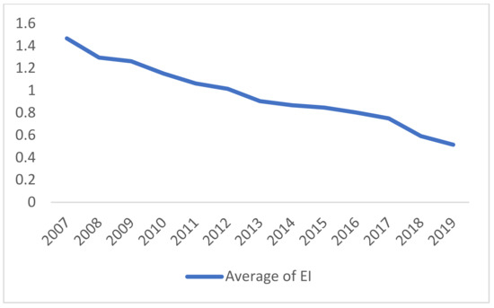
Figure 1.
Average provincial energy intensity in China, 2007–2019.
4.1.2. Descriptions and Source of Explanatory Variables
- (1)
- Financial Development Index (FD)
The financial-related ratio represents the level of regional financial development (FD). The formula for calculating the financial development index is (deposit balance of financial institutions + loan balance of financial institutions)/GDP. The statistics for the measure are derived from the China Statistical Yearbook, the China Financial Statistical Yearbook, and the provincial statistical yearbooks.
Figure 2 reports the average value of China’s provincial financial development index during the reporting period, demonstrating that the extent of provincial financial development in China increased overall during the reporting period.
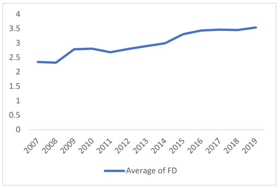
Figure 2.
Average of China’s Provincial Financial Development Index, 2007–2019.
- (2)
- Green Financial Index (GF)
The green financial system consists of four modules: green credit, green investment, green insurance, and government support. Based on the composition of the financial system, the indicator system in Table 1 is developed, which in turn forms a comprehensive measurement system for the level of green financial growth. To overcome the subjectivity of typical expert weight scoring, this paper uses the entropy value approach to give indicator weights objectively. For the variables of the positive influence index system, this paper adopts Equation (1) to standardize them; for the variables of the negative influence index system, this paper adopts Equation (2) to standardize them.

Table 1.
Green financial indicator system for 30 provinces in mainland China.
The term represents the value after regularization of the indicator data, represents the maximum value of the jth indicator data, and represents the minimum value in the jth indicator data.
represents the weight of the jth indicator in the ith year, the is calculated as in Equation (3). The information entropy is calculated as in Equation (4).
The formula for calculating the indicator weights is presented as Equation (5).
By constructing the above index system and using the entropy method, the digital financial index of 30 provinces in mainland China of 13 years is measured. Figure 3 reports the average value of China’s provincial green financial index from 2007 to 2019.
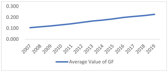
Figure 3.
Annual Average of China’s Provincial Green Financial Index, 2007–2019.
4.1.3. Descriptions and Source of Control Variable
Factors such as human capital investment, fiscal policy, government intervention scale, and industrial scale may have a corresponding impact on the regional energy consumption and total output level; human capital investment (HC), fiscal transparency (FT), industrial SO2 emissions (SDE), and fiscal decentralization (FDA) were selected as control variables in this paper for 30 provinces in mainland China from 2007 to 2019.
- (1)
- Investment in Human Capital (HC)
Using data from the provinces’ statistical yearbooks, the degree of investment in human capital was calculated as the ratio of students enrolled in general secondary schools in the region to the total population of the region.
- (2)
- Fiscal Transparency (FT)
Every year, the Shanghai University of Finance and Economics publishes the “Fiscal Transparency Report.” The report’s “Fiscal Transparency Index” is the most authoritative statistic for gauging fiscal transparency in China at the moment. It is used as a control variable in this paper.
- (3)
- Industrial SO2 emissions (SDE)
The “China Statistical Yearbook” and local statistical yearbooks report the data of this variable in each province in each year. The unit of this data is million tonnes.
- (4)
- Fiscal Decentralization (FDA)
The ratio of a region’s budgetary fiscal revenue to budgetary fiscal spending is employed in this research to measure regional fiscal decentralization [66]. The “China Statistical Yearbook” is used to provide relevant fiscal data.
The descriptive statistics for the explained variables, core explanatory factors, and control variables are shown in Table 2.
Table 2.
Descriptive statistics of the variables.
4.1.4. Spatial Weight Matrix
The spatial weight matrix is a method for quantifying the interrelationships between spatial locations, spatial structural features, and spatial units. Specifically, the spatial weight matrix is a way to quantify the relative spatial location and spatial interaction effects of spatial unit i on spatial unit j in geographic space. In the spatial autoregressive model (SAR), the explained variables generate spatial effects through the spatial weight matrix, thus forming the spatial lag term of the explained variables. In the spatial error model (SEM), the error terms generate spatial effects through the spatial weight matrix, and in the spatial Durbin model (SDM), both the explained and explanatory variables can form spatial lag terms based on the spatial weight matrix.
From the way in which the spatial weight matrix is set up, it can be divided into three main categories: (1) spatial weight matrix based on geographical contiguity; (2) spatial weight matrix based on spatial distance; and (3) spatial weight matrix based on the socio-economic structure. In this paper, we believe that the third setting method is the most scientific one. For example, Shanghai and Beijing Province in China are neither adjacent to nor spatially distant than Shanghai and Anhui Province. However, in terms of economic factors such as population activities and economic exchanges, the economic and social exchanges between Shanghai and Beijing Province are closer than those between Shanghai and Anhui Province. Therefore, the economic spatial weight matrix is constructed as the spatial weight matrix in this paper.
The economic spatial weight matrix can indicate the proximity of economic links across areas and is a useful tool for examining the “spatial impacts” of economic variables between regions with regular economic exchanges. As a result, an economic spatial weight matrix is built in this paper. The matrix is shown in Formula (6).
and represent the average per capita actual outputs of region and region , respectively, from 2007 to 2019.
4.1.5. The Spatial Distribution of Core Variables
Since spatial econometrics is the improvement of traditional econometrics, which neglects spatial autocorrelation and spatial heterogeneity, it is necessary to discuss the spatial autocorrelation and spatial heterogeneity embodied in the panel data of the core variables of this paper. To achieve this, the regional distribution maps of economic variables can visualize the spatial clustering and spatial heterogeneity characteristics of the data. Thus, this paper makes a preliminary judgment on the spatial dependence of economic variables by drawing the regional distribution map of the core variables. Due to space limitations, this paper only reports the regional distribution map of spatially explained variables and spatially explanatory variables in 2007 and 2019. Figure 4 below shows that the core variables all have significant spatial agglomeration.
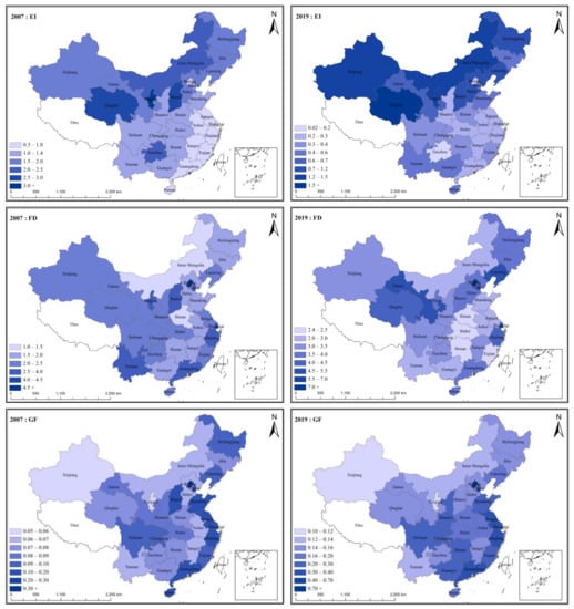
Figure 4.
The spatial and temporal distribution of the core variables for 2007 and 2019.
4.2. Empirical Models
4.2.1. Spatial Econometric Model Construction
In general, the inclusion of typical geospatial features in the data leads to spatial autocorrelation between different observations and spatial heterogeneity in the model, which are generally ignored by traditional econometric methods, violating the classical Gauss Markov assumption. In the econometric approach, since observations are spatially correlated with each other, they are not guaranteed to be independent of each other. The classical Gauss Markov assumption requires that the explanatory variables must be independent of each other during repeated sampling of the sample. Similarly, the presence of spatial heterogeneity makes the homoskedasticity requirement of the error term of the classical assumption impossible to be satisfied. Anselin [67] provided a series of different estimation methods for spatial econometric models to circumvent the spatial autocorrelation problem and the spatial heterogeneity problem that arise in traditional econometrics.
Anselin [68] classified spatial econometric models into spatial autoregressive models (SAR), spatial error models (SEM), and spatial Durbin models (SDM). Among them, the spatial autoregressive model (SAR) considers the interaction of dependent variables between neighboring regions. The spatial error model (SEM) considers the existence of spatial correlation in omitted variables or unobservable random shocks. The economic significance of SEM lies in the fact that shocks occurring in one region are transmitted to neighboring regions with a spatial weight matrix, and this form of transmission has long-term continuity. The spatial Durbin model (SDM) is a general form of the spatial autoregressive model (SEM) and spatial error model, which takes into account the joint effect of spatially lagged explanatory and explained variables on the explained variables.
To verify Hypothesis 1, Hypothesis 2, Hypothesis 4, and Hypothesis 5 in this paper and to study the spatial effects of green finance and financial development on regional energy intensity, this paper constructs a spatial autoregressive model (model 1), spatial error model (model 2), and spatial Durbin model (model 3) based on the study of Le Sage et al. [69] in order to choose a suitable spatial econometric model for the analysis of this paper.
The core variables in the equation are explained in the following section: and are the coefficients of the core explanatory variables. and are the time fixed effect and space fixed effect, respectively. is the spatial weight matrix based on the spatial econometric model of this paper. and are the lagged regression coefficients of the explained variable and explanatory variable. is the set of control variables and their coefficients. Additionally, as the model may have problems such as omitted variables or observation errors, the random error term is set in the model.
4.2.2. Panel Threshold Model Construction
Given the possibility of endogeneity, it is necessary to further investigate the non-linear impact of financial development on regional energy intensity under green finance regulation for Hypothesis 3. The following model 4 was constructed using Hansen’s non-linear static panel threshold model [70], with the green financial index (GF) as the threshold variable and the financial development index (FD) as the core explanatory variable:
In the equation, is the intercept, is the coefficient when the threshold variable is less than the threshold value (), and is the coefficient when the threshold variable is greater than the threshold value (). Additionally, as the model may have problems such as omitted variables or observation errors, the random error term is set in the model.
5. Empirical Results and Analysis
5.1. Spatial Econometric Model Analysis
5.1.1. Spatial Global Moran Index Test
Before analyzing the spatial econometric model, it is necessary to test the spatial applicability of the explained variables and core explanatory variables in this paper. This paper refers to the research of Long, X. et al. [71] and uses global Moran’s I index proposed by Moran to verify the applicability of the model [72]. The expression of the global Moran exponent is shown in Equation (11).
Equation (11) represents the measurement method of the global Moran index (Moran’s I) based on the spatial weight matrix , where if the boundary between the i-th and j-th region exists; if there is no boundary. represents the number of individuals, and represent the variable values in regions and , respectively, and is the mean of the variables.
After the test, based on the economic space weight matrix, the test results of the regional energy intensity (lnEI), the global Moran index of the financial development index (FD), and the green financial index (GF) all rejected the original hypothesis at the 1% level of significance. This shows that the spatial agglomeration of explanatory variables and explained variables in this paper is significant, and it is suitable to use the spatial econometric model. Figure 5 and Figure 6 report the global Moran index status of the explained variables from 2007 to 2019 and Moran scatter plots for the years 2007 and 2019, respectively, proving that the spatial econometric model set in this paper is reasonable.
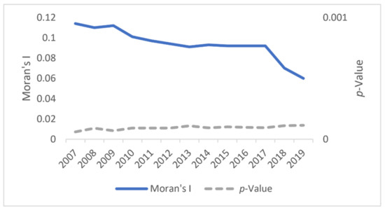
Figure 5.
Global Moran index and significance of provincial energy intensity (lnEI) in China.
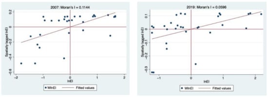
Figure 6.
Moran scatter plot of provincial energy intensity (lnEI) in China in 2007 and 2019.
In Figure 5, the p-value is the result of the statistical test of global Moran’s I, i.e., to determine whether global Moran’s I is significant in a statistical sense, by transforming global Moran’s I into a z-statistic and testing whether it is greater or less than the critical value. The steps are as follows.
First, consider the original hypothesis “” (there is no spatial autocorrelation). Under this original assumption, the expected value of global Moran’s I () is proved to be
Next, the Z-statistic following the asymptotic standard normal distribution is constructed as
As Figure 5 shows, the absolute value of global Moran’s I transformed into the z-statistic value of the explanatory variable lnEI for each year is greater than 2.56, and its corresponding p-value is less than 0.01, indicating that global Moran’s I is significant at the 1% level of significance.
5.1.2. Model Selection and Testing
In order to select the appropriate spatial econometric model from model 3–model 5 and to verify its suitability, this paper refers to the studies of Le Sage et al. [69] and Elhorst [73] and constructs three types of statistics, LR, Wald, and LM, in order to select the model. The effects of the model were evaluated using the LR test and the Hausman test. The results are shown in Table 3.
Table 3.
Model selection and testing.
- (1)
- LM test
For large samples, the Lagrange multiplier test (LM), Wald test, and LR test were equivalent in discriminating the applicability of the spatial econometric models (SAR, SEM, and SDM) and OLS regression models. As for the LM test, Burridge [74] and Anselin [68] proposed the LM-Error test and LM-Lag test, which are alternative tests for spatial error models (SEMs) and spatial autoregressive models (SARs), respectively. Bera and Yoon [75] and Anselin [76,77] then improved on this by proposing the robust LM-Error test (Robust LM-Error) and the robust LM-Lag test (Robust LM-Lag):
In the above equations:
In the equation above, W is the spatial weight matrix, X is the set of variables, m represents the number of explanatory variables, and is the estimated value of the parameter set.
Based on the above discussion and equations, the LM test can be used to assess whether to apply the spatial econometric model. If the spatial econometric model is employed, the next step is to assess the choice between the SEM and SLM. If both LM-Lag and LM-Error are not significant, the traditional OLS regression model is selected; if both are significant, Robust LM-Lag and Robust LM-Error shall be further compared. Based on the test, LM-Lag, LM-Error, Robust LM-Lag, and Robust LM-Error were 168.459, 171.632, 37.250, and 40.423, respectively. The corresponding p-values were less than 0.01. Therefore, the original hypothesis of choosing a non-spatial effect model cannot be accepted, which again proves the choice of the general form of the spatial Durbin model (SDM) that combines both the spatial error model (SEM) and spatial lag model (SLM).
- (2)
- LR test
In the application of spatial econometric models, the likelihood ratio (LR) test can be used to determine whether the corresponding constrained models (SAR and SEM) are approximately equal to the value of the strong likelihood function of the unconstrained model (SDM). Specifically, the first step is to construct the unconstrained model and the constrained model to obtain the maximum likelihood function.
In the equation above, and are the maximum likelihood estimates of the set of parameters and the sum of the variance of the error term for the unconstrained model, respectively. and are the maximum likelihood estimates of the set of parameters and the variance of the error term for the constrained model, respectively. Thus, the LR statistic can be constructed as follows:
For the spatial econometric model, this paper sets two original hypothesis: “” and “”. The first hypothesis states that the meaning of the spatial Durbin model (SDM) can be simplified to the spatial autoregressive model (SAR), and the second hypothesis states that the meaning of the spatial Durbin model (SDM) can be simplified to the spatial error model (SEM).
When , the two original hypotheses are rejected. The alternative test values of 28.79 and 29.90 for SAR and SEM, respectively, both passed the 1% significance level test, indicating that the general form of SDM for SAR and SEM should be used.
In addition, according to the results of LR tests that were carried out once again for individual effects (Ind) and time effects (Time), with coefficients of 566.15 and 48.76, respectively, and both with p-values less than 0.01, the paper should employ the temporal dual fixed effects to estimate the model.
- (3)
- Wald test
The Wald test was described by Agresti [78] and Polit [79] as a method mainly used to test whether the parameters associated with a set of explanatory variables are zero. If the Wald test indicates that these explanatory variables are not significant, they can be omitted from the model.
Elhors [73] suggested the use of the Wald test for spatial econometric models, discriminating whether the spatial Durbin model (SDM) can degenerate into the spatial autoregressive model (SAR) and the spatial error model (SEM) in the spatial econometric model. The Wald test is quite consistent with the likelihood ratio (LR) test—both have the same original hypotheses of “” and “”.
The tested Wald statistics for SAR and SEM were 8.67 and 8.91, respectively, both rejecting the original hypothesis that SDM is not optimal at the 5% significance level. Thus, the spatial Durbin model was once again chosen as the analytical model.
- (4)
- Hausman test
The Hausman test was proposed by Hausman [80]. It is used to determine whether the random effect is correlated with the explanatory variables; if not, then a random effect is used, otherwise it is a fixed effect. The procedure of the Hausman test is shown below:
In the equation above, and are the parameter estimates of fixed effects and random effects, respectively. and are the estimates of the error term variance of the parameter estimates of the fixed effects and random effects, respectively. The original hypothesis of the Hausman test is “”. If the original hypothesis is rejected, the fixed-effects model should be chosen.
In addition, it should be noted that the Hausman test-statistic under the traditional econometric model obeys a distribution with m degrees of freedom, where m is the number of explanatory variables. However, the classical Hausman test does not apply under the perspective of spatial econometrics considering spatial dependence and correlation, because the right-hand side of the spatial econometric model contains spatial lagged terms of the explanatory and explanatory variables. Therefore, it is necessary to consider these spatial lagged terms as explanatory variables and to increase the degrees of freedom, which in turn adjusts the Hausman test to obtain the Hausman test for spatial panels.
However, given geographical dependency and correlation, the traditional Hausman test is not relevant from the perspective of spatial econometrics. In order to test the model r based on the spatial Durbin model, this paper refers to the study of Pace and Le Sage [81] and employs the spatial panel Hausman test. The test results reject the original hypothesis of not using fixed effects (FE), so the fixed effects model is used.
In summary, the spatial Durbin model with spatio–temporal dual fixed effects and fixed effects is used as the regression model for parameter estimation in this paper.
5.1.3. Analysis of the Spatial Econometric Estimation Results
Based on the above test conclusions, this paper constructs a spatial Doberman model for analysis, and the parameter estimation results are shown in Table 4.
Table 4.
Results of parameter estimation for model 1 (spatial Durbin model).
As shown in Table 4, the spatial auto-regressive coefficients of the model all pass the 10% or 5% significance test with values of −0.694, −0.700, −0.706, −0.724, and −0.739, respectively. The results indicate that in the Chinese context, energy intensity has a significant negative spatial spillover effect on itself. In other words, an increase in energy intensity in one province can significantly suppress the province’s economic ties with another. The energy intensity of a province can dramatically suppress the energy intensity of provinces with close economic linkages to that province, indicating that energy intensity has a crowding-out effect on environmentally friendly industries across provinces. The increase in energy intensity is inevitably accompanied by a series of situations that are not conducive to the improvement of environmental and energy efficiency, such as technological progress favoring traditional high energy-consuming industries, industrial structure deviation, and resource mismatch, all of which will inevitably lead to the extrusion of high-tech industries and green technology industries within the region and their concentration in other provinces to suppress the energy intensity of other provinces. Additionally, the estimation results of the spatial autoregressive coefficients can sufficiently prove that Hypothesis 5 is a true statement.
The results of the main effects parameter estimation from the spatial Durbin model show that the coefficients of the financial development index are 0.114, 0.101, 0.101, 0.103, and 0.0985, all of which are significant at the 1 percent level, which is basically consistent with the parameter estimation results of the fixed-effects model. The results indicate that the spatial effect of regional financial development, due to “preference” and “capital market distortions”, has a significant negative effect on regional energy intensity. This result adequately verifies the correctness of Hypothesis 1. The coefficients of the green financial index were significant at the 5% or 1% level of significance, with values of −1.115, −0.832, −0.844, 0.824, and −0.962, respectively, which are basically consistent with the parameter estimation results of the fixed-effect model. This result adequately verifies the correctness of Hypothesis 2. Thus, green finance plays an important role in correcting the negative externalities of financial development as a grip. Moreover, green finance also helps to guide the financial and capital markets to change their capital investment logic, leveraging financial resources to concentrate more on high-tech and green technology industries with long cycles and complex technologies, but supported by national policies. This will therefore create a significant disincentive for regional energy intensity.
The coefficients before W × GF were 3.411, 2.784, 3.557, 3.425, and 7.425, all of which passed the significance test of 5% or 1%. The results indicate that the theoretical mechanism indicated by Hypothesis 5 actually exists in the Chinese context. Based on the economic spatial weight matrix, although the development of green finance has a significant inhibitory effect on the province’s energy intensity, due to the small scale of green finance in China and the existence of phenomena such as “greenwashing” in the financial market, the positive regional externalities of green finance can still not be translated into significant positive spatial externalities through the “diffusion effect” channel. On the other hand, China’s current disorderly competition among regions has resulted in white-hot competition for financial and innovation resources among regions. The competition has gradually evolved into a “zero-sum game” type of regional competition, even though the scale of green finance remains small and the volume is limited, forcing regions to compete for limited green financial resources. This has exacerbated the anarchic competition among areas. As a result, an increase in green finance in one province contributes significantly to the energy intensity of other provinces, diminishing their energy usage efficiency.
The coefficient of W × FD was not significant and had a different sign for a different number of control variables. The result indicates that the mechanism of financial development’s geographical spillover impact was not significant and its externality was not significant while its direction was ambiguous. This is due to two mutually impeding paths of action, the “escapist competition effect” and the “Schumpeterian effect”, that the spatial orientation of financial development has on regional energy intensity, according to the perspective of the spatial spillover and regional competition [82]. Regarding the two actions, the escapist competition follows the logic of “financial development—intensification of regional competition—reduction of innovation rent—an increase in high-tech level—a decrease in energy intensity”. In other words, competition between regions for the financial industry reduces the region’s industrial profit and forces the region to invest financial resources in innovative industries to win in long-term regional competition. The Schumpeter effect follows the logic of “financial development—intensification of regional competition financial development—increased regional competition—inhibition effect of high-tech industries—increased energy intensity”. In other words, financial development intensifies inter-regional financial competition and the innovators are discouraged from entering due to the low profits of regional industries, which is a result of this competition. In addition, the R&D costs and riskiness of high-tech industries are generally high, so the competition suppresses the growth of high-tech industries and green technology industries, resulting in the improvement of regional energy. As a result, the spatial spillover effect of the financial development level on energy intensity was not significant, as both the escapist competition effect and the Schumpeter effect exist locally in the Chinese model under current financial development and regional competition conditions.
5.1.4. Extended Analysis
Since the reform and opening up, China’s regional economic development has always maintained an unbalanced model. That is, there are large differences in the development of China’s mideastern regions and western regions. This difference has produced a great deal of analysis and verification of economic phenomena’ impact. In order to study the regional heterogeneity of the interaction between economic variables, this paper splits the whole sample into mideastern and western regions and estimates the spatial Durbin model once again. The results are shown in Table 5 below.
Table 5.
Spatial Durbin model sub-region parameter estimation results.
- (1)
- The parameter estimation of the spatial Durbin model in the mideastern provinces was basically the same as the estimation results under the full sample, but the spatial spillover effect coefficient of the financial development index of the mideastern provinces was significant at the level of 1%, and the value was −0.786. This result indicates that in the mideastern regions of China, based on the economic space weight matrix, the financial development of a province has a significant negative spatial conduction effect on the energy intensity of other provinces. The reason is the relatively high level of financial development in the mideastern regions, which has formed a clear spatial conduction path and mechanism. From the perspective of the direction of the coefficient, financial development mainly produces evasive competition effects from the perspective of regional competition in the mideastern regions. That is, through regional competition, the regional innovation level is improved and energy utilization efficiency is improved. The negative externalities generated by energy efficiency have a spatial effect consistent with the full sample on local high-tech industries and green technology industries.
- (2)
- The direction of the main effect coefficients in the western region was basically the same as the estimated results under the full sample, but the spatial autoregression of the explained variables in the western region was not significant, indicating that there was no significant spatial spillover effect in the western region. This is because, due to historical reasons and the limited level of economic development, the financial development level of the western region is lagging, financial transactions and factor flows are not active, and the economic exchanges between regions are not as active as those in the mideastern regions, so there is no intra-regional economic exchange, forming a spatial effect.
5.1.5. Robustness Test
- (1)
- Eliminate years that would cause interference
The parameter estimation of the spatial Durbin model in this paper is based on the panel data from 2007 to 2019. During the reporting period, the financial crisis in 2008 forced China to adjust the measures and intensity of financial market supervision, especially China’s macro-prudential supervision of the financial market, which had a profound impact on China’s financial industry and the development of green finance, so the data before 2008 may be different. The sample data of 2007 interfered with the research in this paper to a certain extent, so the sample data of 2007 were excluded in this paper, and the re-estimated results prove the robustness of the research in this paper. Table 6 reports the test results.
Table 6.
Robustness test I: Eliminate years that would cause interference.
- (2)
- Exclude samples from special areas
The research area of this paper includes 30 provinces in mainland China (excluding Tibet), including four municipalities directly under the Central Government, namely, Beijing, Shanghai, Tianjin, and Chongqing. According to the size of the city and its relatively small geographical area compared to other provinces, the flow of financial capital in these regions is smoother than that in other provinces. In addition, Shanghai is the financial center of China, with the most complete financial system and the most active financial market in China, and Beijing also exerts the “headquarter effect” of the financial market, which might interfere with the research. Therefore, this paper excludes samples from these regions, and the estimated results are basically consistent with the above conclusions. Table 7 reports the results.
Table 7.
Robustness test II: exclude samples from special areas.
- (3)
- Addition of possible left out variables
Considering that factors such as industrial scale, government fiscal policy, and human capital may have an impact on regional energy intensity, this paper uses industrial sulfur dioxide emissions (SDE), human capital (HC), fiscal transparency (FT), and fiscal decentralization (FDA) as control variables in its model. In addition, considering factors such as the level of labor input, government intervention, population, and the scale of regional greenery also have an impact on regional energy intensity, the labor force (10,000 people) (Label), government size (GS), population density (km2/person) (PD) and forest cover (Forest) are added to the original model as control variables. Among them, the labor force uses the number of people employed in the three industries at the end of the year as its proxy. The government size is calculated as the local general budget expenditure ratio to regional GDP. The above data were obtained from the China Statistical Yearbook and the statistical yearbooks of each province. After adding these variables, the parameter estimation (reported in Table 8) is consistent with the original, which can prove the robustness of this paper.
Table 8.
Robustness test III: Addition of possible left out variables.
5.2. Panel Threshold Model Analysis
5.2.1. Threshold Effects Test and Determination of Thresholds
In order to verify Hypothesis 3, this paper constructs the threshold effect model (Model 6) and conducts 300 bootstrap self-sampling events under the condition of a triple threshold effect using stata15.1 and determines the threshold degree of the freedom significance test for the threshold variable Green Financial Index (GF). As shown in Table 9, the p-values of the single-threshold effect and the double-threshold effect tests of Model 6 are 0.0033 and 0.0000, respectively, which are both significant. However, the triple-threshold effect fails the significance test, so this paper sets the double-threshold model.
Table 9.
Self-sampling tests for threshold effects.
5.2.2. Analysis of Panel Threshold Regression Results
After the threshold effect test, this paper determines the double threshold values as 0.0910 and 0.1340, respectively, and conducts parameter estimation under the panel threshold effect of the threshold variable Green Financial Index (GF). The results are shown in Table 10.
Table 10.
Analysis of regression results for threshold effects.
Based on Table 10, the paper draws the following conclusions:
It can be seen from the regression results that under the regulation of green finance, financial development has a significant nonlinear effect on regional energy intensity, and the direction of its coefficient changes from positive to negative with the improvement of green finance development level. The effect of regional energy intensity presents an inverted U shape. With the development of green finance, the negative externalities generated by financial development on the level of regional energy utilization and energy efficiency are gradually regulated by green finance and finally reverse the level of regional energy intensity. Green finance is conducive to transforming the investment logic of the financial market, innovating investment, and financing channels, and quickly clearing out the “zombie enterprises” and high-pollution and high-energy-consuming industries that exist in the market due to path dependence and financial oligopoly. This ensures a considerable scale of financial resources and funds to flow into environmentally friendly and energy-saving industries, corrects the misallocation of financial resources caused by traditional financial investment preferences, and alleviates the problem of excessive energy intensity in the region. In terms of the regression coefficients of the financial development index (FD) under different thresholds, the mechanism described by Hypothesis 3 significantly exists.
When the green financial index (GF) is lower than the first threshold value (0.0910), the coefficient of the financial development index (FD) is 0.121, and it is significant at the 5% significance level; at this time, the development level of green finance is low, and the scale is small and cannot have a significant adjustment effect on regional energy intensity. Because the development of green finance has just started, there are more common “greenwashing” and “green bleaching” phenomena, which in turn contribute to the negative externalities of financial development. Therefore, financial development still has a significant positive impact on regional energy intensity at this stage.
When the green financial index (GF) is in the second stage (0.0910 < GF ≤ 0.1340), the coefficient of the financial development index is an insignificant positive number, and its absolute value is smaller than that of the first stage. The development of finance and green finance restrains the negative externalities of financial development. At this point, green finance partially circumvents the capital mismatch caused by financial market investment and financing preferences by amending the financial investment logic and path, making the negative externalities of financial development disappear significantly.
When the green financial index (GF) is above the second threshold (0.1340), the coefficient of financial development is −0.0847 and significant at the 10% level. It means that as the level of green finance continues to rise, it not only corrects the resource mismatch caused by investment preferences but also creates a significant “aggregate investment effect”. A larger green finance industry in the financial market fully mobilizes the positive factors in the financial development process, and the negative externalities of financial development disappear and reverse the regional energy intensity.
6. Conclusions and Policy Recommendations
6.1. Conclusions
Based on the above analysis, this paper draws the following conclusions:
First, financial development has significantly promoted regional energy intensity. Financial development has had a negative impact on regional energy efficiency through capital mismatches caused by investment preferences in non-environmentally friendly industries, as well as oligopoly and capital market distortions in the financial market itself. At the same time, green finance has significantly suppressed regional energy intensity, indicating that green finance has become an important starting point for improving regional energy efficiency by improving regional innovation efficiency, promoting technological progress, leveraging scarce financial resources to agglomerate in green industries and high-tech industries, and comprehensively curbing regional energy intensity.
Secondly, financial development and green finance have a significant joint negative impact on regional energy intensity. Green finance, as a positive factor in the process of financial development, can effectively adjust the negative externalities generated by financial development so that it can reversely inhibit regional energy.
In addition, the spatial effects of regional green financial development are manifested as a “siphon effect” and a “polarization effect”, thereby exacerbating the energy intensity of other provinces through spatial economic activities, while financial development is due to evasive competition effects and Schumpeter’s effects. The two mutually resisting effects of the special effect and the fact that the cross-regional unified financial market in the Chinese context have not yet developed and have not yet formed a significant spatial spillover effect between provinces.
Furthermore, green finance has a significant regulatory effect on the development of negative externalities in finance. At the same time, this regulatory effect is non-linear and will gradually increase with the development of green finance, making financial development subject to the adjustment of green finance. Regional energy intensity has the effect of promoting first and then inhibiting.
Finally, with respect to different geographical divisions, the research in this paper shows a certain range of heterogeneity. In mainland China, the spatial effect of financial development in the mideastern and central regions will significantly inhibit the regional energy intensity. A series of problems have resulted in insignificant spatial effects in the central and western regions.
6.2. Policy Recommendations
Considering the conclusions, the study recommends the following policy suggestions.
The government should continue to promote financial development and sustain the marketization of finance and reduce government intervention. Promoting green finance in the process of financial growth entails breaking the oligopoly of current state-owned commercial banks in the market. Furthermore, the path dependence of traditional high energy-consuming industries caused by excessive government intervention and oligopoly must be broken to quickly clear out the backward production capacity and “zombie enterprises” that have existed for a long time due to this path dependence. Finally, the transformation and upgrading of the regional industrial structure should be fully realized to circumvent the negative externalities of capital market distortions and suppress regional energy intensity entirely.
The government should vigorously support the green finance industry and help green finance to play a leading role in the financial sector. Given the grasping effect of green finance itself on curbing regional energy intensity and the regulatory effect on the negative externalities of financial development, it is necessary to expand the scale of the green finance industry so that it can positively guide the financial sector towards environmentally friendly development to curb regional energy intensity. To meet this requirement, on the one hand, the government should expand the scale of green finance and increase the share of green finance in the capital market through policy tilts. Next, a portion of financial activities that are not conducive to high-quality regional economic development should be regulated or banned. On the other hand, it is also necessary to establish a scientific green finance assessment system, improve and unify the certification standards of the green finance industry represented by green bonds as soon as possible, alert and punish the actions of “greenwashing” and “green bleaching” in the capital market, and maintain the orderly expansion of capital. At the same time, because of the problems including technical complexity, long cycle time, low profitability, high policy risk, and information asymmetry in green finance at this stage, which is potentially contradictory to the inertia of finance in pursuing short-term profits, governments at all levels should also set long-term goals and timetables and vigorously support the green finance industry in terms of funding and policies to avoid short-sightedness.
Given the existing “ polarization effect “ and “ crowding out effect “ between regions, there is a need to construct a mechanism for coordinated and unified development between regions. First, knowledge and technology spillover between regions should be realized, as should the sharing of quality resources; second, inter-regional cooperation and orderly competition should be formed to avoid disorderly competition between regions; and finally, a cross-regional unified financial market should be established, so that green finance and other quality financial resources can spread rapidly through the system, turning the “polarization effect” into a “trickle-down effect”, ultimately curbing energy intensity across China.
The mideastern region should give full play to its technological, financial, and first-mover advantages. First, it should vigorously support the development of green financial industries and green technology industries, strive to avoid the negative externalities of financial development, and introduce policies to guide it to develop in the direction of alleviating energy intensity. The western region should respond positively to the western Development Strategy proposed by the Chinese government. First, it should vigorously develop the financial sector and expand the scale of finance; second, it should support and develop the green financial industry by attracting capital and technology, accepting the capital, knowledge, and technology spillovers from the mideastern region, as well as payment transfers from the central government; finally, it should also strengthen inter-regional exchanges and cooperation to achieve synergistic and integrated regional development.
7. Possible Research Contributions and Shortcomings
7.1. Possible Research Contributions
Using spatial econometric and panel threshold models, this paper provides an in-depth study of the relationship between financial development, green finance, and regional energy intensity in China.
Although many studies have specifically analyzed the dilemma between financial growth and ecology, this paper argues that there are still some gaps in the existing research:
- (1)
- Most of the existing studies argue that financial development can bring abundant funds for the R&D of enterprises. Thus, financial development can improve regional energy efficiently as a whole. This kind of view ignores the “preference mismatch” behavior of financial subjects caused by the oligopoly of Chinese state-owned commercial banks in the financial market and thus underestimates the distortion of financial development in regional energy efficiency.
- (2)
- Most of the existing studies state that green finance can improve the environment and promote economic development in the direction of high quality, which has a positive effect on regional ecological environment improvement and energy intensity mitigation. This view ignores the fact that green finance does not adequately correct the distortion of regional energy efficiency at the early stage of development due to the existing problems and thus ignores the fact that the impact of green finance on energy intensity is actually non-linear.
- (3)
- The two economic factors of financial development and green finance can actually be regarded as “growth and ecology” issues in the financial field. However, few studies have included financial development, green finance, and regional energy intensity in a unified research framework for analysis, and there are gaps in the study of their underlying mechanisms and related findings.
In comparison to existing studies, the paper may have the following marginal contributions:
- (1)
- Reviewing the relationship between regional financial development and regional energy intensity from the perspectives of “preference mismatch” and “capital market distortion,” it is concluded through empirical analysis that under the Chinese system, financial development reinforces regional energy intensity.
- (2)
- The spatial effect of green finance formation has been analyzed and verified through the spatial Durbin model. Existing studies have proved that green finance has mechanisms to mitigate regional energy intensity. On this basis, this paper further proves that green finance in China has a significant spatially reinforcing effect on energy intensity under the distortion of “zero-sum games” and disorderly competition between provinces and regions.
- (3)
- For the first time, financial development, green finance, and regional energy intensity are analyzed in a unified research framework. Through a panel threshold model, this paper investigates the joint mechanism of green finance and financial development with respect to regional energy intensity. It is found that the effect of financial development on regional energy intensity shows an inverted U-shape under the threshold effect of green finance. In addition, this paper also finds that the phenomena of “green washing” and “green bleaching” exist in the early development of green finance, which cannot correct the distortion factors in the process of regional financial development, breaking through the existing research.
- (4)
- Through sub-sample regression and sub-region parameter estimation, it was determined that there are significant differences in financial and green financial development processes between the mideastern regions and the western regions of China. The research provides a reference for policy recommendations for each region, tailored to the local context.
- (5)
- On the basis of mechanism analysis and empirical analysis, policy recommendations are proposed for properly guiding financial development and green finance to jointly promote regional energy efficiency improvement and effectively mitigate regional energy intensity. These recommendations provide relevant references for the government to make decisions at the levels of the marketization process, industrial policy guidance, regional coordination, and localized development.
7.2. Possible Research Shortcomings
The research in this paper has the following shortcomings, which can possibly be improved and addressed by further research:
- (1)
- In terms of regional panel data selection, this paper uses panel data at the provincial level for macro-regional analysis but not at the level of smaller administrative divisions. Since there are a lot of missing data at the prefecture and district levels in China, this data selection is based on data availability. However, this is at fault since it does not provide a thorough examination of the mechanisms relating to financial development, green financing, and energy intensity in China at the prefecture and district levels. On this issue, we consider the use of substitution proxy variables, text analysis, and data mining to address the missing data issue and obtain more detailed analysis results.
- (2)
- In this paper, the relationship between financial development, green finance, and regional energy intensity is examined at a macro level, but in reality, corporations are the primary consumers of energy, and changes in business groups’ energy consumption patterns are directly related to variations in regional energy intensity. We therefore consider obtaining and measuring relevant data from enterprises to fully investigate the mechanisms of financial development, green finance, and energy intensity at the micro level.
- (3)
- Through the use of some findings from related studies, this paper’s mechanism and hypothesis are inferred, which has some persuasive power. In the future, we plan to use rigorous mathematical logic and combine game theory, complex network theory, and other theories to analyze the specific mechanism of the research object in this paper, so as to strengthen mechanism analysis in mathematical language, making mechanism analysis more convincing.
Author Contributions
Conceptualization, K.L. and J.P.; methodology, software, validation, formal analysis, and writing—original draft preparation, K.L. and S.Y.; investigation, and resources, D.F. and J.W.; writing—review and editing, and supervision, J.P. and C.W. All authors have read and agreed to the published version of the manuscript.
Funding
This research was supported by the General Scientific Research Project of Zhejiang Provincial Department of Education (Y202044040), the Academy of Longyuan Construction Financial Research in Ningbo University (LYZDB2005), the Advanced Humanities and Social Sciences Cultivation Program of Ningbo University (XPYQ21005), the Zhejiang Provincial Philosophy and Social Science Planning Project (19XXJC02ZD-2), and the Research Project of Ningbo Cross-Strait Integration Development Institute (2021NBTY06).
Institutional Review Board Statement
Not applicable.
Informed Consent Statement
Not applicable.
Data Availability Statement
The authors would like to thank the editors and anonymous reviewers for their thoughtful and constructive comments.
Conflicts of Interest
The authors declare no conflict of interest.
References
- Mardani, A.; Streimikiene, D.; Cavallaro, F. Carbon dioxide (CO2) emissions and economic growth: A systematic review of two decades of research from 1995 to 2017. Sci. Total. Environ. 2019, 649, 31–49. [Google Scholar] [CrossRef] [PubMed]
- Ren, S.; Hao, Y.; Wu, H. The role of outward foreign direct investment (OFDI) on green total factor energy efficiency: Does institutional quality matters? Evidence from China. Resour. Policy 2022, 76, 102–114. [Google Scholar] [CrossRef]
- Yang, S.; Su, X.; Ran, Q. Assessing the impact of energy internet and energy misallocation on carbon emissions: New insights from China. Environ. Sci. Pollut. Res. 2021, 29, 23436–23460. [Google Scholar] [CrossRef] [PubMed]
- Li, B.; Wu, J.; Chen, S. Urbanization, industrialization, informatization, and energy intensity in China. Chin. Popul. Resour. Environ. 2015, 25, 69–76. [Google Scholar]
- Chang, M. Energy intensity, target level of energy intensity, and room for improvement in energy intensity: An application to the study of regions in the EU. Energ. Policy 2014, 67, 648–655. [Google Scholar] [CrossRef]
- Jiang, X.; Duan, Y.; Green, C. Regional disparity in energy intensity of China and the role of industrial and export structure. Resour. Conserv. Recycl. 2017, 120, 209–218. [Google Scholar] [CrossRef]
- Ana, F.; Manuel, D.; Jorge De, B.; Ricardo, M. Relating carbon and energy intensity of best-performing retailers with policy, strategy, and building practice. Energy Effic. 2020, 13, 597–619. [Google Scholar]
- Hamidi, S.; Benabdeljlil, N. Managerial and technological innovations: Any relationship? Procedia-Soc. Behav. Sci. 2015, 181, 286–292. [Google Scholar] [CrossRef][Green Version]
- Yang, X. Spatial effects of financial scale and financial structure on technological innovation of enterprises. In Proceedings of the 2019 4th International Conference on Financial Innovation and Economic Development, Sanya, China, 4 February 2019. [Google Scholar]
- Ren, S.; Hao, Y.; Wu, H. How does green investment affect environmental pollution? Evidence from China. Environ. Resour. Econ. 2022, 81, 25–51. [Google Scholar] [CrossRef]
- Park, K. Testing for competition in the South Korean and Chinese commercial banking markets. Asia-Pac. J. Financ. Stud. 2013, 42, 56–75. [Google Scholar] [CrossRef]
- Zhou, X.; Pei, Z.; Qin, B. Assessing market competition in the Chinese banking industry based on a conjectural variation model. China World Econ. 2021, 29, 73–98. [Google Scholar] [CrossRef]
- Treado, C. Pittsburgh’s evolving steel legacy and the steel technology cluster. Camb. J. Reg. Econ. Soc. 2010, 3, 105–120. [Google Scholar] [CrossRef]
- Islam, F.; Shahbaz, M.; Ahmed, A. Financial development and energy consumption nexus in Malaysia: A multivariate time series analysis. Econ. Model. 2013, 30, 435–441. [Google Scholar] [CrossRef]
- Mahalik, M.; Babu, M.; Loganathan, N. Does financial development intensify energy consumption in Saudi Arabia? Renew. Sustain. Energy Rev. 2017, 75, 1022–1034. [Google Scholar] [CrossRef]
- Salahuddin, M.; Gow, J.; Ozturk, I. Is the long-run relationship between economic growth, electricity consumption, carbon dioxide emissions and financial development in Gulf Cooperation Council Countries robust? Renew. Sustain. Energy Rev. 2015, 51, 317–326. [Google Scholar] [CrossRef]
- Dogan, E.; Seker, F. The influence of real output, renewable and non-renewable energy, trade and financial development on carbon emissions in the top renewable energy countries. Renew. Sustain. Energy Rev. 2016, 60, 1074–1085. [Google Scholar] [CrossRef]
- Shahbazet, M.; Solarin, S.; Mahmood, H.; Arouri, M. Does financial development reduce CO2 emissions in the Malaysian economy? A Time Series Analysis. Econ. Model. 2013, 35, 145–152. [Google Scholar] [CrossRef]
- Tamazian, A.; Chousa, J.; Vadlamannati, K. Does higher economic and financial development lead to environmental degradation? Evidence from BRIC countries. Energy Policy 2009, 37, 246–253. [Google Scholar] [CrossRef]
- Sun, P.; Wang, Y.; Cen, Y. Does financial development affect the structure of energy consumption? A cross-country empirical analysis. Nankai Econ. Res. 2011, 2, 28–41. [Google Scholar]
- Kong, Y.; Wei, F. Financial development, financial structure and carbon emission. Environ. Eng. Manag. J. 2017, 16, 1609–1622. [Google Scholar]
- Xiang, X.; Yang, G.; Sun, H. The impact of the digital economy on low-carbon, inclusive growth: Promoting or restraining. Sustainability 2022, 14, 7187. [Google Scholar] [CrossRef]
- Lagoardesegot, T. Sustainable finance. A critical realist perspective. Res. Int. Bus. Financ. 2019, 47, 1–9. [Google Scholar] [CrossRef]
- Wang, C.; Dong, G. Research on green financial ecology construction based on low carbon economy. Ekoloji 2019, 28, 3635–3641. [Google Scholar]
- Weber, W.; Domazlicky, B. Does environmental protection lead to slower productivity growth in the chemical industry. Environ. Resour. Econ. 2004, 28, 301–324. [Google Scholar]
- Zhang, K.; Chen, H.; Tang, L. Green finance, innovation and the energy-environment-climate nexus. Front. Environ. Sci. 2022, 10, 87–99. [Google Scholar] [CrossRef]
- Yu, C.; Wu, X.; Zhang, D. Demand for green finance: Resolving financing constraints on green innovation in China. Energy Policy 2021, 153, 112–125. [Google Scholar] [CrossRef]
- He, L.; Gan, S.; Zhong, T. The impact of green credit policy on firms’ green strategy choices: Green innovation or green-washing? Environ. Sci. Pollut. Res. 2022, 10, 107–116. [Google Scholar] [CrossRef]
- Yu, J.; Fu, J. Credit rationing, innovation, and productivity: Evidence from small and medium-sized enterprises in China. Econ. Model. 2021, 97, 220–230. [Google Scholar] [CrossRef]
- Parekh, N.; Attuel, L. Social entrepreneurship finance: The gaps in an innovative discipline. Int. J. Entrep. Behav. Res. 2021, 28, 135–155. [Google Scholar] [CrossRef]
- Chava, S.; Nanda, V.; Xiao, S. Lending to innovative firms. Rev. Corp. Financ. Stud. 2017, 6, 234–289. [Google Scholar] [CrossRef]
- Feng, G.; Serletis, A. Undesirable outputs and a primal Divisia productivity index based on the directional output distance function. J. Econom. 2014, 183, 135–146. [Google Scholar] [CrossRef]
- Tone, K. A slacks-based measure of efficiency in data envelopment analysis. Eur. J. Oper. Res. 2001, 130, 498–509. [Google Scholar] [CrossRef]
- Fatih, K.; Yasser, Y. Is technological change biased toward energy? A multi-sectoral analysis for the French economy. Energy Policy 2009, 38, 1842–1850. [Google Scholar]
- Stigler, G. Monopoly and oligopoly by merger. Am. Econ. Rev. 2009, 5, 23–34. [Google Scholar]
- Haltiwanger, J.; Harrington, J. The impact of cyclical demand movements on collusive behaviour. Rand. J. Econ. 2010, 22, 89–106. [Google Scholar] [CrossRef]
- Dong, M.; Stella, H.; Sun, H.; Zhou, C. A macroeconomic theory of banking oligopoly. Eur. Econ. Rev. 2020, 138, 103–126. [Google Scholar] [CrossRef]
- Hu, K.; Shi, D. The impact of government-enterprise collusion on environmental pollution in China. J. Environ. Manag. 2021, 292, 112–119. [Google Scholar] [CrossRef]
- Lee, J. Green finance and sustainable development goals: The case of China. J. Asian Financ. Econ. 2020, 7, 577–586. [Google Scholar] [CrossRef]
- Palencia, J.; Furubayashi, T.; Toshihiko, N. Analysis of CO2 emissions reduction potential in secondary production and semi fabrication of non-ferrous metals. Energy Policy 2013, 52, 328–341. [Google Scholar] [CrossRef]
- Sheinbaum, C.; Ruiz, B.; Ozawa, L. Energy consumption and related CO2 emissions in five Latin American countries: Changes from 1990 to 2006 and perspectives. Energy Policy 2011, 36, 3629–3638. [Google Scholar] [CrossRef]
- Steckel, J.; Jakob, M. The role of financing cost and de-risking strategies for clean energy investment. Int. Econ. 2018, 155, 19–28. [Google Scholar] [CrossRef]
- Tao, H.; Zhuang, S.; Xue, R.; Cao, W.; Tian, J.; Shan, Y. Environmental finance: An interdisciplinary review. Technol. Forecast. Soc. 2022, 179, 121–149. [Google Scholar] [CrossRef]
- Climent, F.; Soriano, P. Green and good? The investment performance of US environmental mutual funds. J. Bus. Ethics. 2011, 103, 275–287. [Google Scholar] [CrossRef]
- Sinha, A.; Mishra, S.; Sharif, A.; Yarovaya, L. Does green financing help to improve environmental & social responsibility? Designing SDG framework through advanced quantile modeling. J. Environ. Manag. 2021, 292, 112–123. [Google Scholar]
- Tu, Q.; Mo, J.; Liu, Z.; Gong, C.; Fan, Y. Using green finance to counteract the adverse effects of COVID-19 pandemic on renewable energy investment-The case of offshore wind power in China. Energy Policy 2021, 158, 123–136. [Google Scholar] [CrossRef]
- Zheng, G.; Siddik, A.; Masukujjaman, M.; Fatema, N. Factors affecting the sustainability performance of financial institutions in Bangladesh: The role of green finance. Sustainability 2021, 13, 10165. [Google Scholar] [CrossRef]
- Arif, A.; Hieu, V.; Ma, C.; Leow, W.; Md, I.; Gniewko, N. Natural resources commodity prices volatility and economic performance: Evaluating the role of green finance. Resour. Policy 2022, 76, 102–143. [Google Scholar] [CrossRef]
- Leiter, M.; Parolini, A.; Winner, H. Environmental regulation and investment: Evidence from European industry data. Ecol. Econ. 2011, 70, 759–770. [Google Scholar] [CrossRef]
- Sun, Z.; Zhang, W. Do government regulations prevent greenwashing? An evolutionary game analysis of heterogeneous enterprises. J. Clean. Prod. 2019, 231, 1489–1502. [Google Scholar] [CrossRef]
- Orman, C. Organization of innovation and capital markets. N. Am. J. Econ. Financ. 2015, 33, 94–114. [Google Scholar] [CrossRef][Green Version]
- Zhu, N.; Bu, Y.; Jin, M.; Mbroh, N. Green financial behavior and green development strategy of Chinese power companies in the context of carbon tax. J. Clean. Prod. 2020, 245, 118–127. [Google Scholar] [CrossRef]
- Campbell, J. A note on the notion of growth pole. Growth. Chang. 2006, 5, 43–45. [Google Scholar] [CrossRef]
- Ozkaya, A. R&D team’s competencies, innovation, and growth with knowledge information flow. IEEE Trans. Eng. Manag. 2010, 57, 416–429. [Google Scholar]
- Theophile, T.; Dienei, M. Polarization patterns in economic development and innovation. Struct. Chang. Econ. Dyn. 2012, 23, 421–436. [Google Scholar]
- Hu, D.; Qiu, L.; She, M.; Wang, Y. Sustaining the Sustainable Development: How do Firms Turn Government Green Subsidies into Financial Performance Through Green Innovation? Bus. Strategy Environ. 2021, 30, 2271–2292. [Google Scholar] [CrossRef]
- Jayaram, R.; Singh, S. Sustainable finance: A systematic review. Int. J. Indian Cult. Bus. Manag. 2020, 1, 317–399. [Google Scholar] [CrossRef]
- Falcone, P. Environmental regulation and green investments: The role of green finance. Int. J. Green Econ. 2020, 14, 159–173. [Google Scholar] [CrossRef]
- Han, C.; Gu, Z.; Yang, H. Investigate the effects of industrial agglomeration on nitrogen dioxide pollution using spatial panel Durbin and panel threshold models. Front. Environ. Sci. 2022, 10, 338–347. [Google Scholar] [CrossRef]
- Yue, Y.; Tian, L.; Yue, Q. Spatiotemporal variations in energy consumption and their influencing factors in China based on the integration of the DMSP-OLS and NPP-VIIRS nighttime light datasets. Remote Sens. 2020, 12, 1151. [Google Scholar] [CrossRef]
- Zhang, J.; Wang, J.; Yang, X.; Ren, S.; Ran, Q.; Hao, Y. Does local government competition aggravate haze pollution? A new perspective of factor market distortion. Socio-Econ. Plan. Sci. 2021, 76, 119–126. [Google Scholar] [CrossRef]
- Liu, H.; Song, Y. Financial development and carbon emissions in China since the recent world financial crisis: Evidence from a spatial-temporal analysis and a spatial Durbin model. Sci. Total Environ. 2020, 715, 136–145. [Google Scholar] [CrossRef]
- Zhang, H.; Ke, H. Spatial spillover effects of directed technical change on urban carbon intensity, based on 283 cities in China from 2008 to 2019. Int. J. Environ. Res. Public Health 2022, 19, 1679. [Google Scholar] [CrossRef]
- Liu, J.; Li, X.; Zhong, S. Does innovation efficiency promote energy consumption intensity? New evidence from China. Energy Rep. 2022, 8, 426–436. [Google Scholar] [CrossRef]
- Tajudeen, I.; Wossink, A. The underlying trend of OPEC energy intensity and the environmental implications. OPEC Eng. Rev. 2020, 44, 63–65. [Google Scholar] [CrossRef]
- Bai, J.; Lu, J. Research on the mechanism of fiscal decentralization’s impact on environmental pollution. J. Polit. Econ. 2017, 10, 37–56. [Google Scholar]
- Anselin, L.; Rey, S. Properties of tests for spatial dependence in linear regression. Geogr. Anal. 1991, 23, 112–131. [Google Scholar] [CrossRef]
- Anselin, L. Lagrange multiplier test diagnostics for spatial dependence and spatial heterogeneity. Geogr. Anal. 1988, 20, 1–17. [Google Scholar] [CrossRef]
- Le, S.; Pace, R. Introduction to spatial econometrics. J. Reg. Sci. 2010, 5, 1014–1015. [Google Scholar]
- Hansen, B. Threshold effects in non-dynamic panels: Estimation, testing, and inference. J. Econom. 1999, 10, 101–117. [Google Scholar] [CrossRef]
- Long, X.; Zhu, Y.; Cai, W.; Li, S. An empirical analysis of tax competition among county governments in China based on the spatial econometric model. Econ. Res. 2014, 49, 41–53. [Google Scholar]
- Moran, P. Notes on continuous stochastic phenomena. Biometrika 1950, 37, 17–23. [Google Scholar] [CrossRef]
- Elhorst, J. Matlab software for spatial panels. Int. Regional Sci. Rev. 2014, 37, 389–405. [Google Scholar] [CrossRef]
- Burridge, P. On the Cliff-Ord test for spatial autocorrelation. J. R. Stat. Soc. B 1980, 42, 107–108. [Google Scholar]
- Bera, A.; Yoon, M. Specification testing with locally misspecified alternatives. Econ. Theory 1993, 9, 649–658. [Google Scholar] [CrossRef]
- Anselin, L.; Bera, A.K.; Florax, R.; Mann, J.Y. Simple diagnostic tests for spatial dependence. Reg. Sci. Urban Econom. 1996, 26, 77–104. [Google Scholar] [CrossRef]
- Anselin, L. A Companion to Theoretical Econometrics; Blackwell Publishing Ltd: Malden, MA, USA, 2001; pp. 310–330. [Google Scholar]
- Agresti, A. Categorical Data Analysis; John Wiley and Son: New York, NY, USA, 1990. [Google Scholar]
- Polit, D. Data Analysis and Statistics for Nursing Research; Appleton & Lange: Stamford, CT, USA, 1996. [Google Scholar]
- Hausman, J. Specification tests in econometrics. Econometrica 1978, 46, 1251–1271. [Google Scholar] [CrossRef]
- Pace, R.; Le, S. A spatial Hausman test. Econ. Lett. 2008, 101, 282–284. [Google Scholar] [CrossRef]
- Li, Q. The view of technological innovation in coal industry under the vision of carbon neutralization. Int. J. Coal Sci. Technol. 2021, 8, 1197–1207. [Google Scholar] [CrossRef]


Publisher’s Note: MDPI stays neutral with regard to jurisdictional claims in published maps and institutional affiliations. |
© 2022 by the authors. Licensee MDPI, Basel, Switzerland. This article is an open access article distributed under the terms and conditions of the Creative Commons Attribution (CC BY) license (https://creativecommons.org/licenses/by/4.0/).