
Optimization of Ground Control Point Distribution for Unmanned Aerial Vehicle Photogrammetry for Inaccessible Fields

 , , ,
, , ,
Abstract
:1. Introduction
2. Materials and Methods
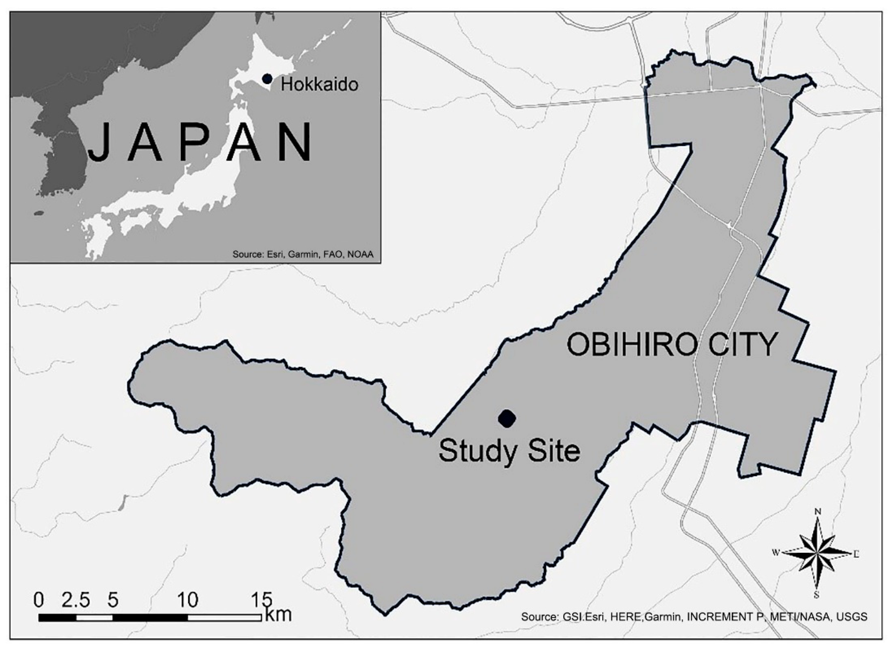
2.1. Study Area
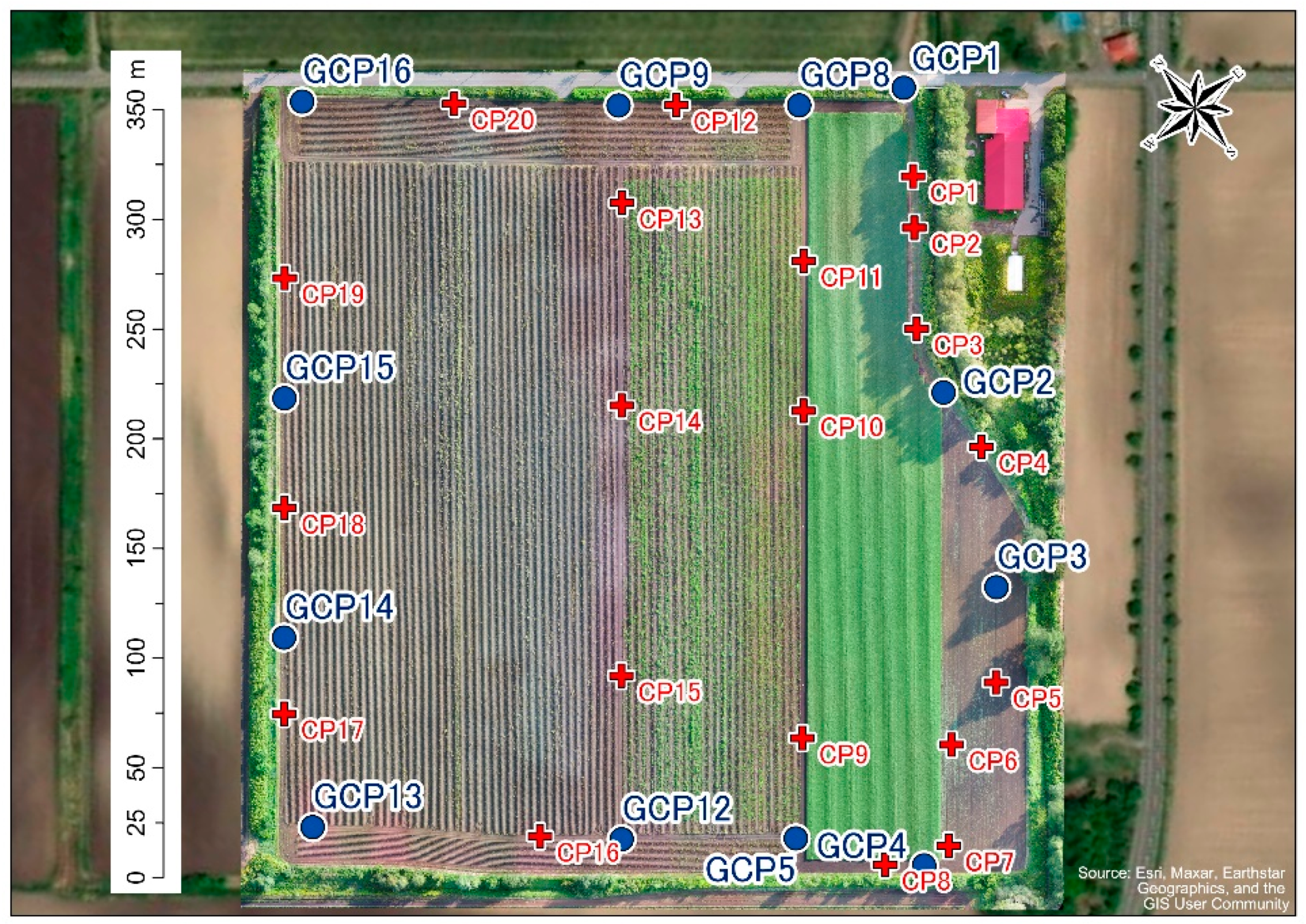
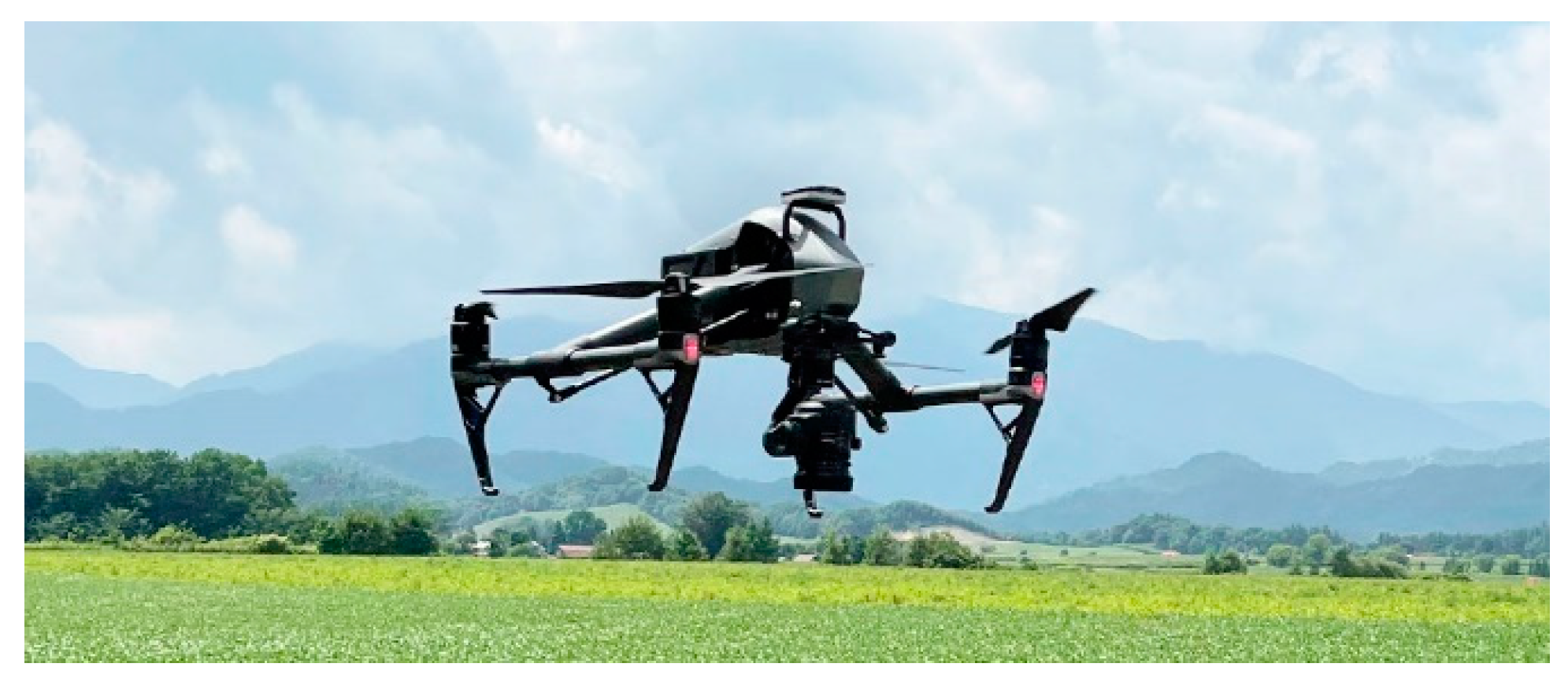
2.2. Data Collection
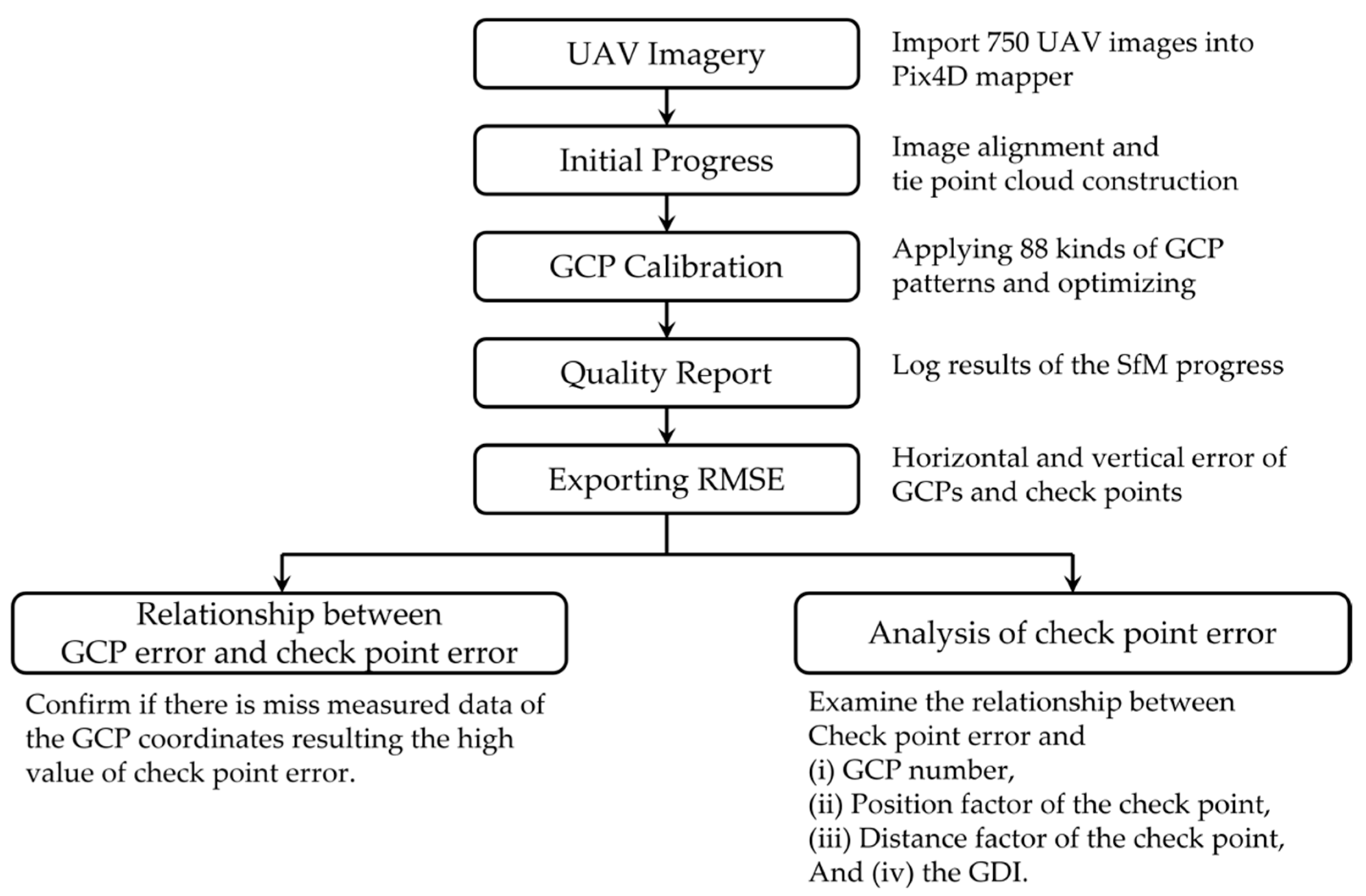
2.3. Data Processing
2.3.1. Workflow
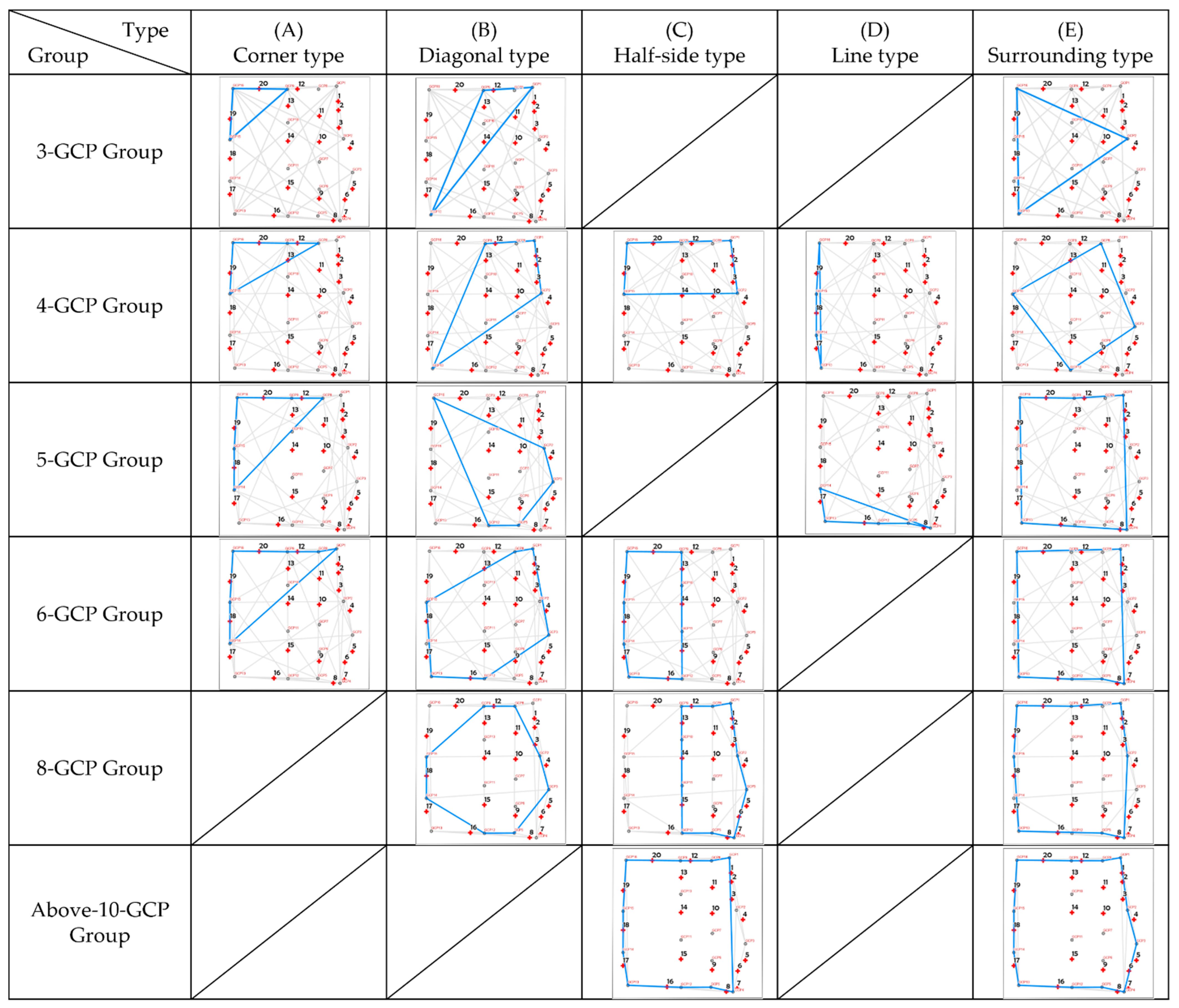
2.3.2. GCP Patterns
2.3.3. GCP Distribution Index Calculation
3. Results
3.1. Relationship between GCP Error and Check Point Error
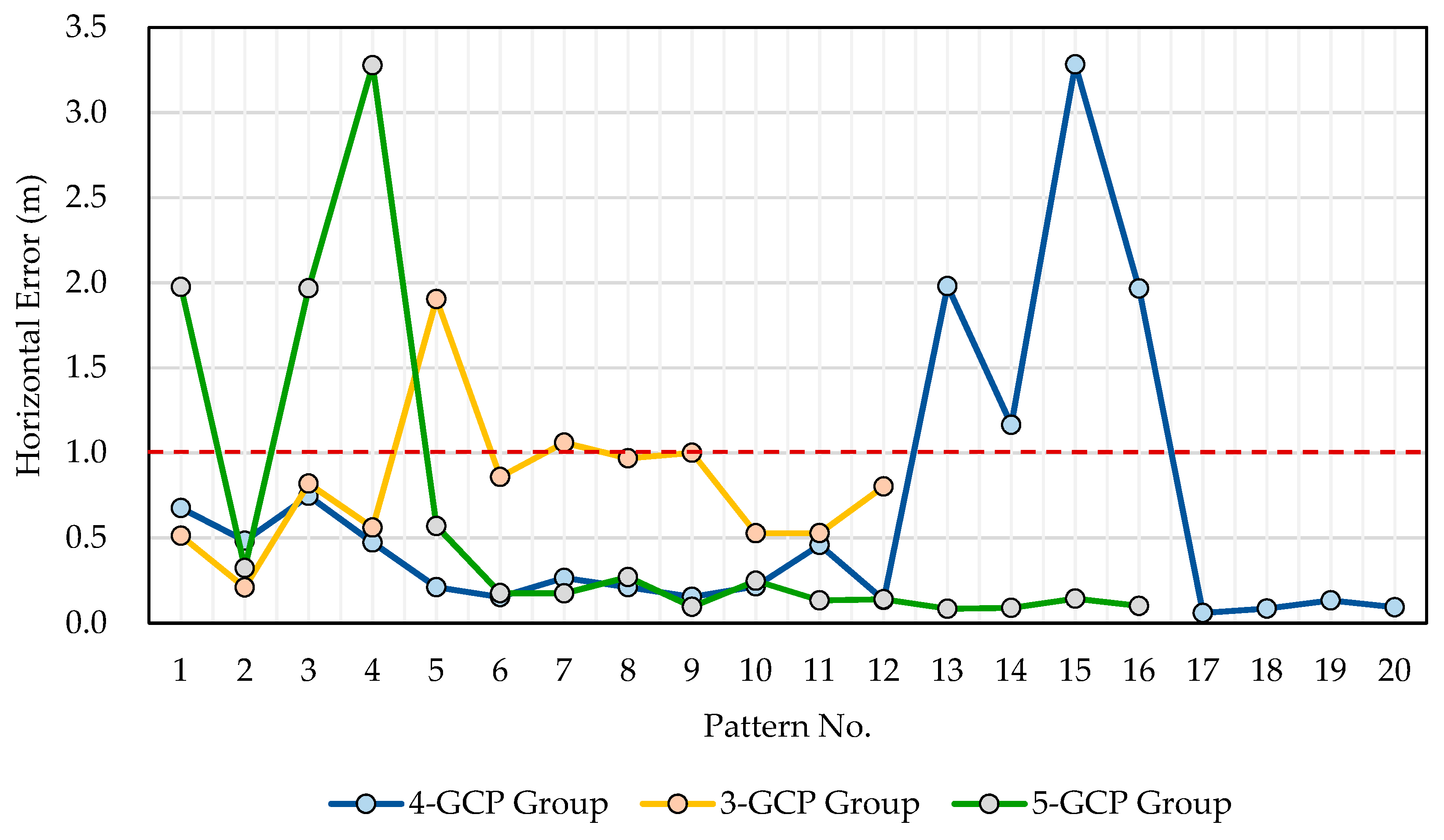
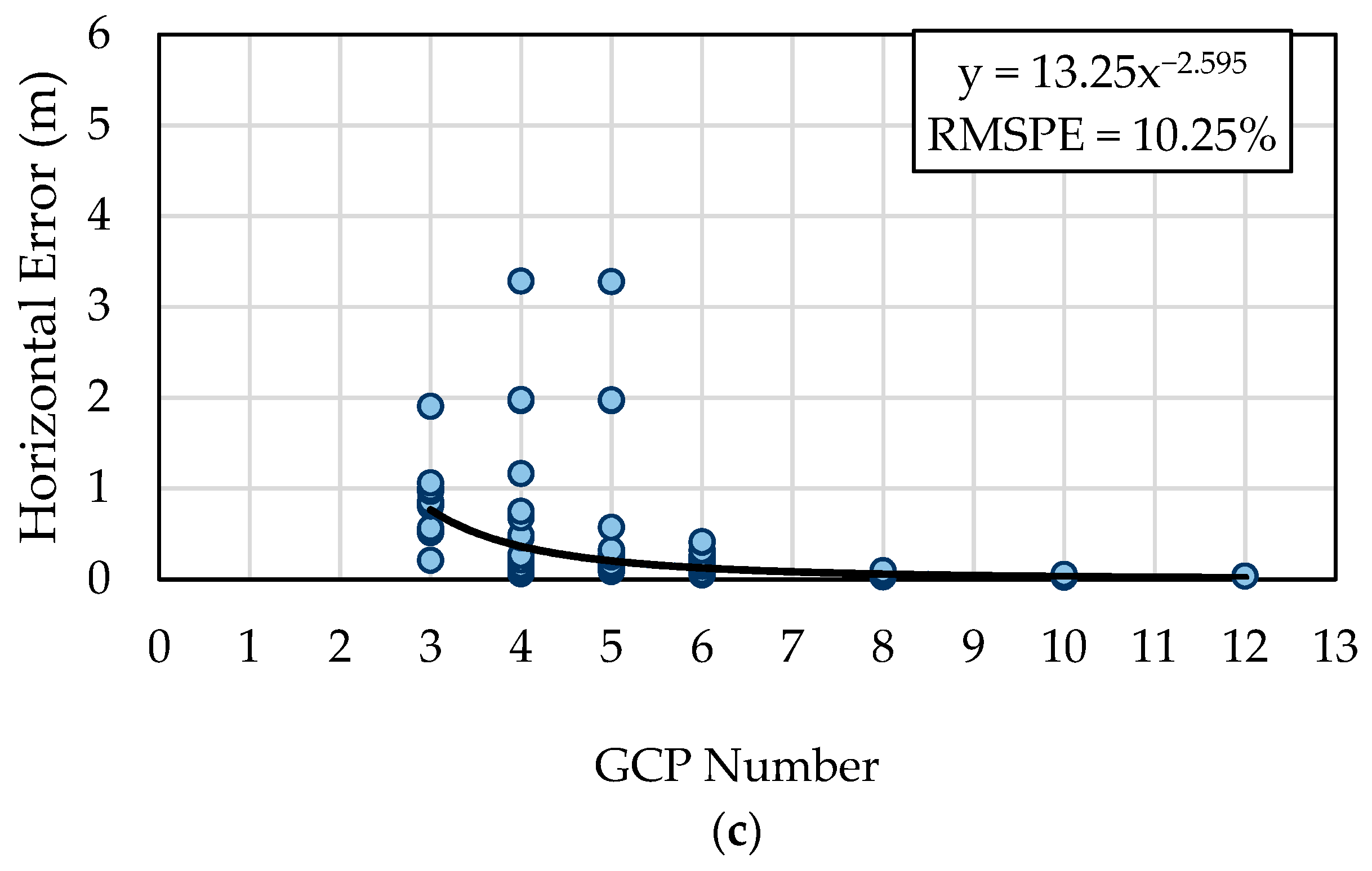
3.2. Relationship between GCP Number and Check Point Error
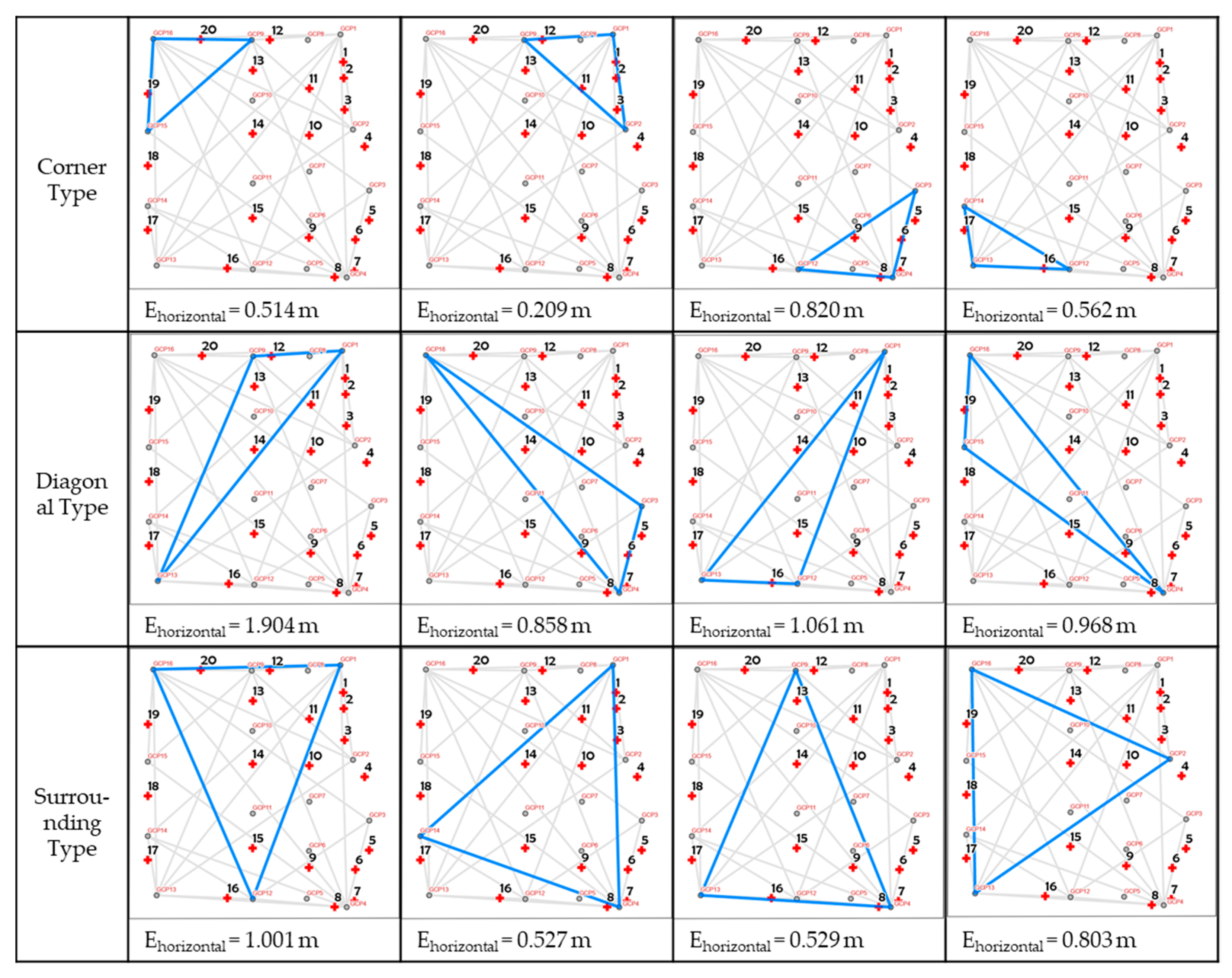
3.3. Relationship between GCP Configuration Type and Check Point Error
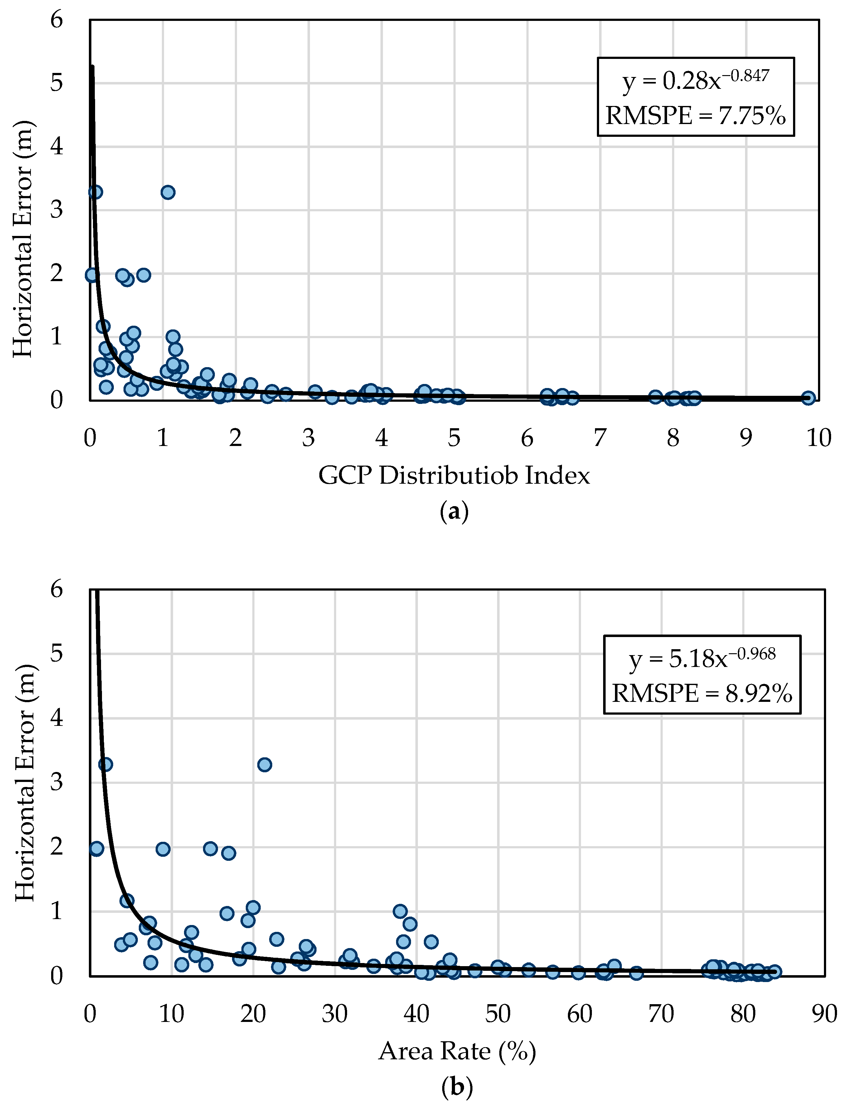
3.4. Describing the Calibration Ability of GCPs by GDI
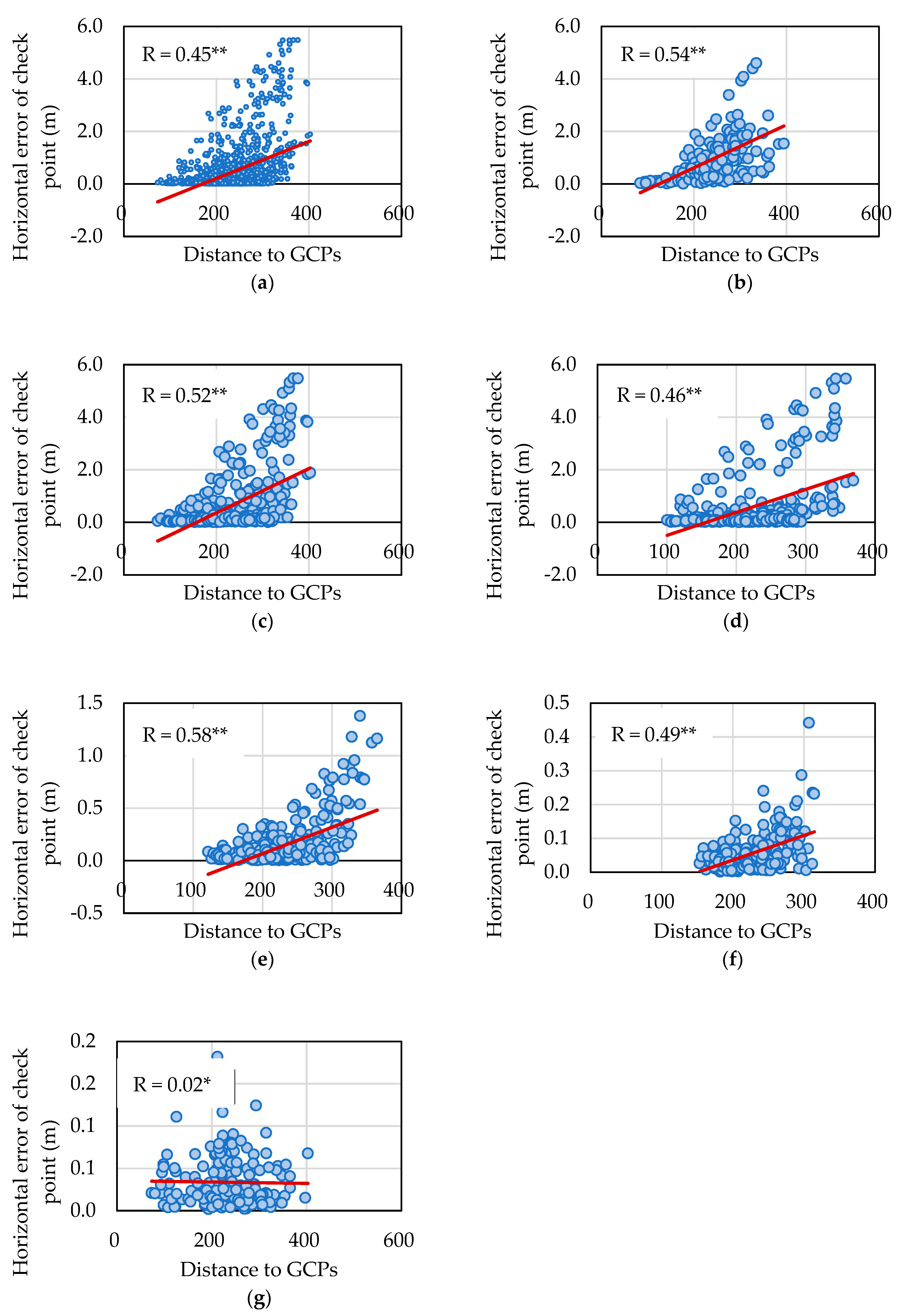
3.5. Relationship between the Position of Check Point Distance and Check Point Error
4. Discussion
5. Conclusions
Author Contributions
Funding
Institutional Review Board Statement
Informed Consent Statement
Data Availability Statement
Acknowledgments
Conflicts of Interest
Abbreviations
| Acronyms | Complete Expression |
| UAV | Unmanned Aerial Vehicle |
| GPS | Global Positioning System |
| GCP | Ground Control Point |
| SfM | Structure from Motion |
| PPK | Post Processing Kinematic |
| RTK | Real Time Kinematic |
| GNSS | Global Navigation Satellite System |
| NRTK | Network Real Time Kinematic |
| GAM | Generalized Additive Model |
| RMSE | Root Mean Square Error |
| MAE | Mean Absolute Error |
| DEM | Digital Elevation Model |
| DSM | Digital Surface Model |
| GDI | GCP Distribution Index |
| STDEV | Standard Deviation |
| RMSPE | Root Mean Squared Percentage Error |
References
- Piras, M.; Taddia, G.; Forno, M.G.; Gattiglio, M.; Aicardi, I.; Dabove, P.; Lo Russo, S.; Lingua, A. Detailed geological mapping in mountain areas using an unmanned aerial vehicle: Application to the Rodoretto Valley, NW Italian Alps. Geomat. Nat. Hazards Risk 2017, 8, 137–149. [Google Scholar] [CrossRef]
- Manfreda, S.; McCabe, M.F.; Miller, P.E.; Lucas, R.; Pajuelo Madrigal, V.; Mallinis, G.; Dor, E.B.; Helman, D.; Estes, L.; Ciraolo, G.; et al. On the use of unmanned aerial systems for environmental monitoring. Remote Sens. 2018, 10, 641. [Google Scholar] [CrossRef] [Green Version]
- Bendig, J.; Yu, K.; Aasen, H.; Bolten, A.; Bennertz, S.; Broscheit, J.; Gnyp, M.L.; Bareth, G. Combining UAV-based plant height from crop surface models, visible, and near infrared vegetation indices for biomass monitoring in barley. Int. J. Appl. Earth Obs. Geoinf. 2015, 39, 79–87. [Google Scholar] [CrossRef]
- Bareth, G.; Bendig, J.; Tilly, N.; Hoffmeister, D.; Aasen, H.; Bolten, A. A comparison of UAV-and TLS-derived plant height for crop monitoring: Using polygon grids for the analysis of crop surface models (CSMs). Photogramm. Fernerkund. Geoinf. 2016, 2016, 85–94. [Google Scholar] [CrossRef] [Green Version]
- Zhang, K.; Tsuji, O.; Kimura, M.; Muneoka, T.; Hoshiyama, K. Monitoring of Crop Plant Height Based on DSM Data Obtained by Small Unmanned Vehicle Considering the Difference of Plant Shapes. Int. J. Environ. Rural. Dev. 2020, 11, 131–136. [Google Scholar]
- Zhang, Y.; Wu, H.; Yang, W. Forests growth monitoring based on tree canopy 3D reconstruction using UAV aerial photogrammetry. Forests 2019, 10, 1052. [Google Scholar] [CrossRef] [Green Version]
- Zhang, Y.; Yang, W.; Zhang, W.; Yu, J.; Zhang, J.; Yang, Y.; Lu, Y.; Tang, W. Two-step ResUp&Down generative adversarial network to reconstruct multispectral image from aerial RGB image. Comput. Electron. Agric. 2022, 192, 106617. [Google Scholar]
- Zhang, Y.; Yang, W.; Sun, Y.; Chang, C.; Yu, J.; Zhang, W. Fusion of multispectral aerial imagery and vegetation indices for machine learning-based ground classification. Remote Sens. 2021, 13, 1411. [Google Scholar] [CrossRef]
- Zhang, W.; Gao, F.; Jiang, N.; Zhang, C.; Zhang, Y. High-Temporal-Resolution Forest Growth Monitoring Based on Segmented 3D Canopy Surface from UAV Aerial Photogrammetry. Drones 2022, 6, 158. [Google Scholar] [CrossRef]
- Sankey, T.; Donager, J.; McVay, J.; Sankey, J.B. UAV lidar and hyperspectral fusion for forest monitoring in the southwestern USA. Remote Sens. Environ. 2017, 195, 30–43. [Google Scholar] [CrossRef]
- Martinez, J.G.; Gheisari, M.; Alarcón, L.F. UAV integration in current construction safety planning and monitoring processes: Case study of a high-rise building construction project in Chile. J. Manag. Eng. 2020, 36, 05020005. [Google Scholar] [CrossRef]
- Zheng, H.; Cheng, T.; Zhou, M.; Li, D.; Yao, X.; Tian, Y.; Cao, W.; Zhu, Y. Improved estimation of rice aboveground biomass combining textural and spectral analysis of UAV imagery. Precis. Agric. 2019, 20, 611–629. [Google Scholar] [CrossRef]
- Guan, S.; Fukami, K.; Matsunaka, H.; Okami, M.; Tanaka, R.; Nakano, H.; Sakai, T.; Nakano, K.; Ohdan, H.; Takahashi, K. Assessing Correlation of High-Resolution NDVI with Fertilizer Application Level and Yield of Rice and Wheat Crops Using Small UAVs. Remote Sens. 2019, 11, 112. [Google Scholar] [CrossRef] [Green Version]
- Hildmann, H.; Kovacs, E. Using unmanned aerial vehicles (UAVs) as mobile sensing platforms (MSPs) for disaster response, civil security and public safety. Drones 2019, 3, 59. [Google Scholar] [CrossRef] [Green Version]
- James, M.R.; Robson, S.; d’Oleire-Oltmanns, S.; Niethammer, U. Optimising UAV topographic surveys processed with structure-from-motion: Ground control quality, quantity and bundle adjustment. Geomorphology 2017, 280, 51–66. [Google Scholar] [CrossRef] [Green Version]
- Bendig, J.; Bolten, A.; Bareth, G. 4 UAV-based Imaging for Multi-Temporal, very high Resolution Crop Surface Models to monitor Crop Growth Variability. Unmanned Aer. Veh. (UAVs) Multi-Temporal Crop Surf. Model. 2013, 44, 53–69. [Google Scholar]
- Yang, J.; Li, X.; Luo, L.; Zhao, L.; Wei, J.; Ma, T. New Supplementary Photography Methods after the Anomalous of Ground Control Points in UAV Structure-from-Motion Photogrammetry. Drones 2022, 6, 105. [Google Scholar] [CrossRef]
- Taddia, Y.; Stecchi, F.; Pellegrinelli, A. Coastal mapping using DJI Phantom 4 RTK in post-processing kinematic mode. Drones 2020, 4, 9. [Google Scholar] [CrossRef] [Green Version]
- Žabota, B.; Kobal, M. Accuracy assessment of uav-photogrammetric-derived products using PPK and GCPs in challenging terrains: In search of optimized rockfall mapping. Remote Sens. 2021, 13, 3812. [Google Scholar] [CrossRef]
- Hugenholtz, C.; Brown, O.; Walker, J.; Barchyn, T.; Nesbit, P.; Kucharczyk, M.; Myshak, S. Spatial accuracy of UAV-derived orthoimagery and topography: Comparing photogrammetric models processed with direct geo-referencing and ground control points. Geomatica 2016, 70, 21–30. [Google Scholar] [CrossRef]
- Fazeli, H.; Samadzadegan, F.; Dadrasjavan, F. Evaluating the Potential of RTK-UAV for Automatic Point Cloud Generation in 3D Rapid Mapping. Int. Arch. Photogramm. Remote Sens. Spat. Inf. Sci. 2016, 41, 221–226. [Google Scholar] [CrossRef] [Green Version]
- Štroner, M.; Urban, R.; Reindl, T.; Seidl, J.; Brouček, J. Evaluation of the georeferencing accuracy of a photogrammetric model using a quadrocopter with onboard GNSS RTK. Sensors 2020, 20, 2318. [Google Scholar] [CrossRef] [PubMed] [Green Version]
- Taddia, Y.; González-García, L.; Zambello, E.; Pellegrinelli, A. Quality assessment of photogrammetric models for façade and building reconstruction using DJI Phantom 4 RTK. Remote Sens. 2020, 12, 3144. [Google Scholar] [CrossRef]
- Teppati Losè, L.; Chiabrando, F.; Giulio Tonolo, F. Boosting the timeliness of UAV large scale mapping. Direct georeferencing approaches: Operational strategies and best practices. ISPRS Int. J. Geo-Inf. 2020, 9, 578. [Google Scholar] [CrossRef]
- James, M.R.; Robson, S. Mitigating systematic error in topographic models derived from UAV and ground—Based image networks. Earth Surf. Processes Landf. 2014, 39, 1413–1420. [Google Scholar] [CrossRef] [Green Version]
- Nikolakopoulos, K.G.; Kyriou, A.; Koukouvelas, I.K. Developing a Guideline of Unmanned Aerial Vehicle’s Acquisition Geometry for Landslide Mapping and Monitoring. Appl. Sci. 2022, 12, 4598. [Google Scholar] [CrossRef]
- Meinen, B.U.; Robinson, D.T. Mapping erosion and deposition in an agricultural landscape: Optimization of UAV image acquisition schemes for SfM-MVS. Remote Sens. Environ. 2020, 239, 111666. [Google Scholar] [CrossRef]
- Tonkin, T.N.; Midgley, N.G. Ground-control networks for image based surface reconstruction: An investigation of optimum survey designs using UAV derived imagery and structure-from-motion photogrammetry. Remote Sens. 2016, 8, 786. [Google Scholar] [CrossRef] [Green Version]
- Bolkas, D. Assessment of GCP number and separation distance for small UAS surveys with and without GNSS-PPK positioning. J. Surv. Eng. 2019, 145, 04019007. [Google Scholar] [CrossRef]
- Mesas-Carrascosa, F.J.; Rumbao, I.C.; Berrocal, J.A.B.; Porras, A.G.F. Positional quality assessment of orthophotos obtained from sensors onboard multi-rotor UAV platforms. Sensors 2014, 14, 22394–22407. [Google Scholar] [CrossRef]
- Ulvi, A. The effect of the distribution and numbers of ground control points on the precision of producing orthophoto maps with an unmanned aerial vehicle. J. Asian Archit. Build. Eng. 2021, 20, 806–817. [Google Scholar] [CrossRef]
- Liu, X.; Lian, X.; Yang, W.; Wang, F.; Han, Y.; Zhang, Y. Accuracy assessment of a UAV direct georeferencing method and impact of the configuration of ground control points. Drones 2022, 6, 30. [Google Scholar] [CrossRef]
- Sanz-Ablanedo, E.; Chandler, J.H.; Rodríguez-Pérez, J.R.; Ordóñez, C. Accuracy of unmanned aerial vehicle (UAV) and SfM photogrammetry survey as a function of the number and location of ground control points used. Remote Sens. 2018, 10, 1606. [Google Scholar] [CrossRef] [Green Version]
- Nagendran, S.K.; Tung, W.Y.; Ismail, M.A.M. Accuracy assessment on low altitude UAV-borne photogrammetry outputs influenced by ground control point at different altitude. In IOP Conference Series: Earth and Environmental Science, Proceedings of the 9th IGRSM International Conference and Exhibition on Geospatial & Remote Sensing (IGRSM 2018), Kuala Lumpur, Malaysia, 24–25 April 2018; IOP Publishing: Bristol, UK; Volume 169, p. 012031.
- Park, J.W.; Yeom, D.J. Method for establishing ground control points to realize UAV-based precision digital maps of earthwork sites. J. Asian Archit. Build. Eng. 2022, 21, 110–119. [Google Scholar] [CrossRef]
- Awasthi, B.; Karki, S.; Regmi, P.; Dhami, D.S.; Thapa, S.; Panday, U.S. Analyzing the Effect of Distribution Pattern and Number of GCPs on Overall Accuracy of UAV Photogrammetric Results. In Lecture Notes in Civil Engineering, Proceedings of the International Conference on Unmanned Aerial System in Geomatics, Roorkee, India, 6–7 Apil 2019; Jain, K., Khoshelham, K., Zhu, X., Tiwari, A., Eds.; Springer: Cham, Switzerland; pp. 339–354.
- Mirko, S.; Eufemia, T.; Alessandro, R.; Giuseppe, F.; Umberto, F. Assessing the Impact of the Number of GCPS on the Accuracy of Photogrammetric Mapping from UAV Imagery. Balt. Surv. 2019, 10, 43–51. [Google Scholar]
- Cabo, C.; Sanz-Ablanedo, E.; Roca-Pardiñas, J.; Ordóñez, C. Influence of the number and spatial distribution of ground control points in the accuracy of uav-sfm dems: An approach based on generalized additive models. IEEE Trans. Geosci. Remote Sens. 2021, 59, 10618–10627. [Google Scholar] [CrossRef]
- Villanueva, J.K.S.; Blanco, A.C. Optimization of ground control point (GCP) configuration for unmanned aerial vehicle (UAV) survey using structure from motion (SFM). Int. Arch. Photogramm. Remote Sens. Spat. Inf. Sci. 2019, 42, 167–174. [Google Scholar] [CrossRef] [Green Version]
- Geographical Survey Institute. Manual of Public Surveying with UAV; Ministry of Land, Infrastructure, Transport and Tourism of Japan: Tokyo, Japan, 2017; pp. 23–24.
- Gindraux, S.; Boesch, R.; Farinotti, D. Accuracy assessment of digital surface models from unmanned aerial vehicles’ imagery on glaciers. Remote Sens. 2017, 9, 186. [Google Scholar] [CrossRef] [Green Version]
- Yang, H.; Li, H.; Gong, Z.; Dai, W.; Lu, S. Relations between the Number of GCPs and Accuracy of UAV Photogrammetry in the Foreshore of the Sandy Beach. J. Coast. Res. 2020, 95, 1372–1376. [Google Scholar] [CrossRef]


| X (m) | Y (m) | Z (m) | |
|---|---|---|---|
| GCP 01 | −139,952.522 | −102,272.435 | 256.863 |
| GCP 02 | −140,070.595 | −102,347.832 | 256.432 |
| GCP 03 | −140,154.070 | −102,386.420 | 258.195 |
| GCP 04 | −140,230.000 | −102,493.170 | 261.535 |
| GCP 05 | −140,182.974 | −102,530.043 | 262.111 |
| GCP 06 | −140,131.528 | −102,482.524 | 260.648 |
| GCP 07 | −140,076.385 | −102,436.148 | 259.196 |
| GCP 08 | −139,928.018 | −102,314.091 | 256.773 |
| GCP 09 | −139,875.156 | −102,377.220 | 257.424 |
| GCP 14 | −139,962.953 | −102,649.875 | 260.426 |
| GCP 15 | −139,879.514 | −102,579.624 | 260.368 |
| GCP 16 | −139,781.105 | −102,486.545 | 258.573 |
| Check Point 01 | −139,986.148 | −102,295.145 | 255.291 |
| Check Point 02 | −140,004.484 | −102,309.756 | 255.227 |
| Check Point 03 | −140,040.503 | −102,338.486 | 255.722 |
| Check Point 04 | −140,100.647 | −102,350.477 | 256.539 |
| Check Point 05 | −140,187.101 | −102,414.480 | 259.264 |
| Check Point 06 | −140,195.925 | −102,448.142 | 260.514 |
| Check Point 07 | −140,230.253 | −102,478.878 | 261.134 |
| Check Point 08 | −140,218.267 | −102,506.576 | 261.775 |
| Check Point 09 | −140,149.903 | −102,498.298 | 261.168 |
| Check Point 10 | −140,035.921 | −102,402.136 | 258.011 |
| Check Point 11 | −139,983.693 | −102,358.083 | 257.232 |
| Check Point 12 | −139,892.041 | −102,356.891 | 257.200 |
| Check Point 13 | −139,910.263 | −102,404.505 | 258.142 |
| Check Point 14 | −139,980.764 | −102,464.030 | 259.577 |
| Check Point 15 | −140,075.091 | −102,543.271 | 261.686 |
| Check Point 16 | −140,107.254 | −102,618.705 | 263.118 |
| Check Point 17 | −139,989.584 | −102,672.110 | 260.428 |
| Check Point 18 | −139,917.891 | −102,611.724 | 260.960 |
| Check Point 19 | −139,837.641 | −102,544.269 | 259.622 |
| Check Point 20 | −139,826.454 | −102,434.035 | 257.530 |
| Rank No. | Horizontal Error (m) | GDI | Area Percentage | GCP Number |
|---|---|---|---|---|
| 10-cm-Rank | 0.060 | 5.360 | 71% | 7 |
| 20-cm-Rank | 0.148 | 2.330 | 47% | 5 |
| 30-cm-Rank | 0.313 | 1.220 | 25% | 5 |
| 40-cm-Rank | 0.689 | 0.654 | 20% | 3 |
| 50-cm-Rank | 1.958 | 0.483 | 13% | 4 |
| 3-GCP Group | 4-GCP Group | 5-GCP Group | 6-GCP Group | 8-GCP Group | Above-10-GCP Group | |
|---|---|---|---|---|---|---|
| Outside | 0.873 | 0.769 | 0.449 | 0.218 | 0.074 | 0.035 |
| Inside | 0.728 | 0.125 | 0.128 | 0.083 | 0.054 | 0.031 |
| Between | 0.247 | 0.118 | 0.06 | 0.062 | 0.037 | 0.027 |
Publisher’s Note: MDPI stays neutral with regard to jurisdictional claims in published maps and institutional affiliations. |
© 2022 by the authors. Licensee MDPI, Basel, Switzerland. This article is an open access article distributed under the terms and conditions of the Creative Commons Attribution (CC BY) license (https://creativecommons.org/licenses/by/4.0/).
Share and Cite
Zhang, K.; Okazawa, H.; Hayashi, K.; Hayashi, T.; Fiwa, L.; Maskey, S. Optimization of Ground Control Point Distribution for Unmanned Aerial Vehicle Photogrammetry for Inaccessible Fields. Sustainability 2022, 14, 9505. https://doi.org/10.3390/su14159505
Zhang K, Okazawa H, Hayashi K, Hayashi T, Fiwa L, Maskey S. Optimization of Ground Control Point Distribution for Unmanned Aerial Vehicle Photogrammetry for Inaccessible Fields. Sustainability. 2022; 14(15):9505. https://doi.org/10.3390/su14159505
Chicago/Turabian StyleZhang, Ke, Hiromu Okazawa, Kiichiro Hayashi, Tamano Hayashi, Lameck Fiwa, and Sarvesh Maskey. 2022. "Optimization of Ground Control Point Distribution for Unmanned Aerial Vehicle Photogrammetry for Inaccessible Fields" Sustainability 14, no. 15: 9505. https://doi.org/10.3390/su14159505