Article

Optimal Scheduling of Thermoelectric Coupling Energy System Considering Thermal Characteristics of DHN

1
College of Information Science and Engineering, Northeastern University, Wenhua Road, NO. 3-11, Shenyang 110819, China
2
Key Laboratory of Integrated Energy Optimization and Secure Operation of Liaoning Province, Northeastern University, Shenyang 110819, China
3
State Grid Jibei Electric Power Co. Ltd., Tangshan Power Supply Company, Jianshe Road, NO. 7, Tangshan 063000, China
4
State Grid Liaoning Electric Power Co. Ltd., Shenyang 110006, China
*
Author to whom correspondence should be addressed.
Sustainability 2022, 14(15), 9764; https://doi.org/10.3390/su14159764
Submission received: 29 May 2022 / Revised: 17 July 2022 / Accepted: 4 August 2022 / Published: 8 August 2022

Abstract

:
In a thermoelectric coupling energy system, renewable energy is often curtailed by the uncertainty of the power generation. Besides, the integration of renewable energy is restricted by the inflexible operation of combined heat and power units due to the strong coupling relationship between power generation and heating supply, especially in winter. Utilization of the district heating network, a heat storage feature, is a cost-effective measure to improve the overall system operational flexibility. In this paper, a new heat characteristic index is proposed in a district heating system, which is applied to measure the impact of the flexibility of combined heat and power units’ output. Furthermore, in order to increase the reliability of an electric power system, a probabilistic model of combined heat and power units’ spinning reserves capacity related to confidence level K is established. What is more, the two indexes K and thermal characteristic index have a coupled relationship. In addition, for model solving methodology, the discretized step transformation and constant mass flow and variables temperature method is adopted to transform the non-linear system model into linear programming form. Case studies are carried out to show the linkage between system costs, K and thermal characteristic index. The optimal result can achieve balance among the system reliability, flexibility and economy.

1. Introduction

With the increase in renewable energy penetration rate, the reliability of a district energy system cannot be guaranteed because the output power of renewable energy, such as solar energy and wind energy, is uncertain and intermittent [1,2,3]. In the northeastern part of China, wind farms produced almost 20% less electricity on account of wind power curtailment, and the uncertainty of the wind energy results in low reliability in an electric power system (EPS). Besides, the proportion of heat supply units in combined heat and power (CHP) units is high due to the long winter heating period [4]. Therefore, to satisfy the high heat load level, coal-fired CHP plants are the main sources for providing load demands of district heating in winter, which still occupies an irreplaceable position in generator units. However, the poor inflexibility of CHP units increases the difficulty of regulating power and heat output. Therefore, to increase the flexibility of CHP units, the district heating system (DHN) participates in the heat regulation of DHS, which plays the role of a heat storage device [5]. Therefore, how to balance the system reliability and unit flexibility scale in a thermoelectric coupling energy system (TCES) has become an important research topic.
A significant number of methods have been presented to improve the system reliability and cope with the renewable energy system (RES) intermittent output [6,7,8]. In [6], a four-level multiagent system is used to implement hierarchical management and hybrid control in a top-down sequence. In [7], the design of robust H∞ controllers for uncertain networked control systems (NCSs) with the effects of both the network-induced delay and data dropout taken into consideration is presented. In [8], a distributed cooperative control for frequency and voltage stability and power sharing in microgrid considering the limitation of communication network. In [9], by modeling the uncertainty of spinning reserves provided by energy storage and traditional power plant with chance-constrained, the fluctuation of RES output and load demand is offset by the rotation reserve capacity. However, how to improve the reliability of TCES has not been mentioned. Wen S. et al. proposed a hybrid multi-objective particle swarm optimization method to minimize the cost of the power system and improve the system voltage stability with consideration of uncertainties in wind power production in [10]. In addition, this paper proposed a probabilistic cost analysis method aiming at EPS optimization. In [11,12], a multi-objective performance index including voltage profile and energy losses indices is utilized in objective function as the standard to measure the system stability and reliability. Therefore, how to build a probabilistic model to measure the reliability of TCES is a matter to be solved.
In recent years, extensive work has been conducted on the coordinated optimization of integrated electrical and heating systems [13,14,15,16,17]. Due to the close linkage between electricity and heating in winter, the inflexible operation of CHP units may limit wind power integration. Using the heat storage capacity of DHN is a cost-efficient measure that can improve the operational flexibility of the energy system to accommodate a large amount of variable wind energy [18,19]. A dynamic state-estimate model for a combined heat and power system is formulated considering the energy storage of both pipelines in the DHN and heat storage tanks; this is formulated as a convex quadratic program in [20], which is solved in a decentralized manner using optimality condition decomposition. In addition, the time delay of DHN and indoor temperature usually affects the operation plan of the DHS heavily. Therefore, a practical CHP-DHS model and multiregional coordinated operation strategy based on model predictive control are developed for planning and operating this CHP system in [21]. It can be seen from the above-mentioned studies that taking full advantage of the heat storage features of DHN to assist CHP units has become an important direction for the district energy systems. However, the above-mentioned studies have not considered to give a specific quantitative value of DHN’s heat release or absorption, nor provide an index to measure the impact of the heat storage characteristics of DHN on the flexibility of the heat regulation capacity of CHP units.
In order to relieve the above-mentioned constraints, an optimal scheduling model which focuses on considering the influence of the quantified heat absorption or release capacity of DHN on the heat regulation flexibility of DHS and the probabilistic constraint of CHP’s spinning reserve capacity is used to improve the reliability of system. The aim is to develop a method that can convert a non-linear model into a linear form with the purpose of minimizing the costs and improving the system’s reliability and flexibility. The main contributions of this paper are described as follows.
(1)
In TCES, a new thermal characteristic index (TCI) based on quantized heat storage capacity of DHN is proposed to measure the DHN’s heat endothermic and exothermic ability to improve the heat regulation flexibility of DHS.
(2)
By controlling confidence level K in the proposed probabilistic constraint of CHP’s spinning reserve capacity, the reliability of the TCES is improved.
(3)
This is the first time the wind power generation uncertainty and DHN’s heat storage capability have been addressed simultaneously in the TCES dispatching problem. Furthermore, this involved converting a non-linear model into a linear form by discretized step transformation and the CF-VT method for the overall problem-solving process.
The remainder of this paper is organized as follows. Section 2 describes the TCES model consisting of EPS and DHS. In Section 3, a coordinated operation approach is proposed and the optimization model is described in detail, with its solution methodology. In Section 4, comparative case studies are carried out to find the optimal operation result. Conclusions are drawn in Section 5.

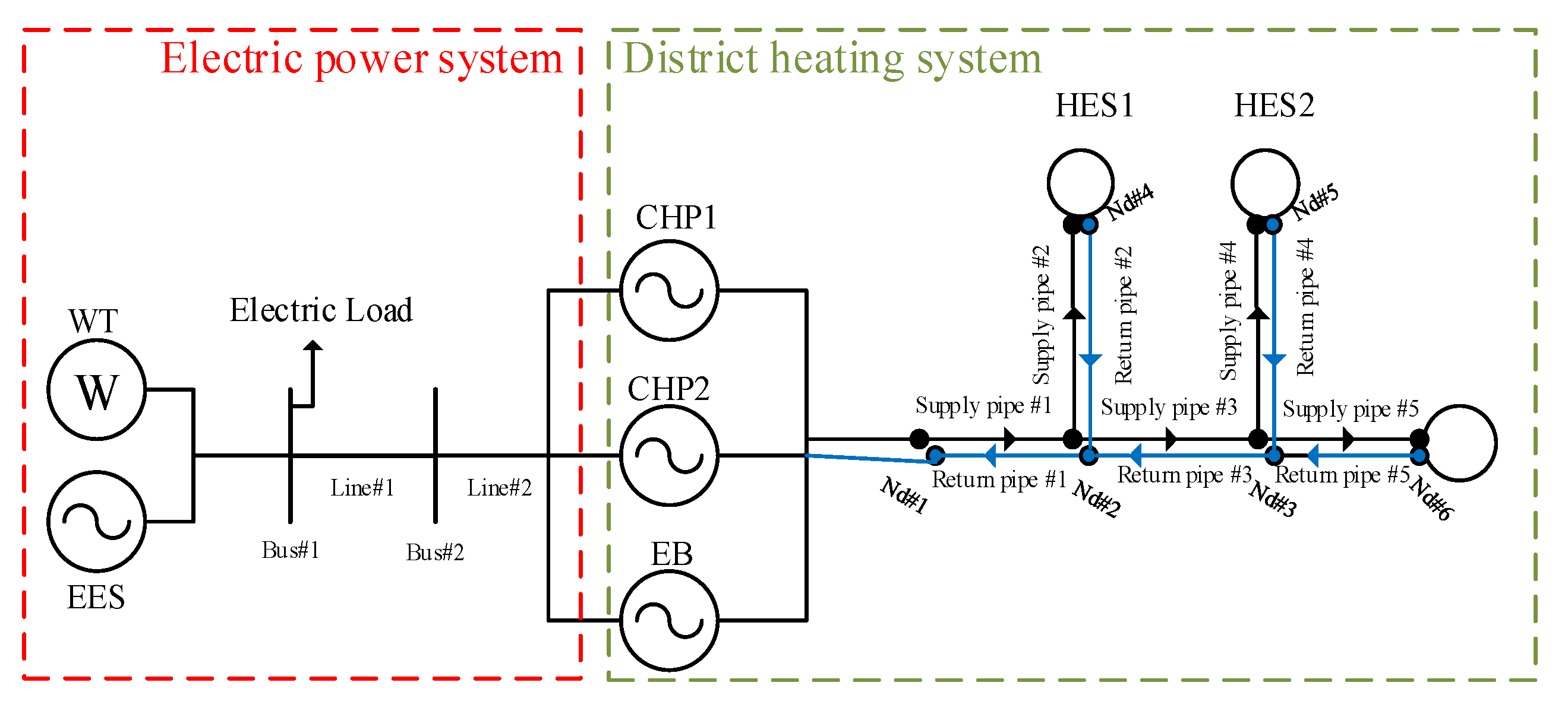
2. Modeling of Thermoelectric Coupling Energy System

In this paper, the TCES model is composed of EPS and DHS. The EPS consists of wind turbines (WT), CHP units, electric energy storage (EES) and electric boiler (EB) devices. The DHS is composed of pipeline networks, heat loads and heat sources (HS) including CHP and EB.

2.1. Probabilistic Model of EPS Considering Confidence Level K

To achieve thermoelectric decoupling and improve the flexibility of the power supply, EB and EES are essential in district energy systems [22]. However, due to the inherently intermittent nature of WT, the operation of EPS is vulnerable to uncertain power exchange between the generation and the load, and hence the operation reliability and supply security are difficult to be guaranteed [23]. Therefore, it is essential to deal with the problem of power generation uncertainties in EPS optimal dispatch to improve the reliability of EPS. In this paper, a probabilistic model of EPS with a reliability constraint is built as follows.
Previous research has shown that wind speeds follow Weibull distribution. The probabilistic density function (PDF) of the wind turbine power output fw(Pw) and the charging or discharging power P t E E S of EES at time t can be found in [24]. Moreover, the changing load injection PL is an important source of uncertainty in the actual power system. A widely used normal distribution model proposed in [9] is used to simulate load fluctuations in this paper. The PDF of power load injection f l ( P L ) is also shown in [9]. In order to promote the combination of multiple random variables, the power of EL (equivalent load) is defined as the difference between the load power and the power output of WT (wind turbine), which is expressed as follows:
P E L = P L P w
where PEL denotes the power of the EL.
In this paper, due to adding EB into the EPS, the operation area of the CHP unit is expanded, and the lower limit of CHP unit’s output power changes. The detailed model about CHP is introduced in Section 2.2.2 and the operation region of CHP is shown in Figure 4. Correspondingly, the spinning reserve constraint is as follows:
P t C H P , M i n P t E B P t C H P + R t C H P P t C H P , M a x
where R t C H P is the power reserve capacity of the CHP unit and P t C H P is the power generated by the CHP unit used to meet power load demands. Besides, P t C H P + R t C H P is the total power generated by the CHP unit. P t E B is the power consumed by the EB device. In addition, the specific expression of P t C H P , M a x and P t C H P , M i n is shown in 6 and 7.
To maintain the power balance, the total rotation reserve provided by CHP is used to compensate for the difference between the fluctuating EL power and its expected value E ( P t E L ) . The expression of E ( P t E L ) is as follows:
E ( P t E L ) = i b , t = 0 N b , t i b , t q b ( i b , t ) i a , t = 0 N a , t i a , t q a ( i a , t )
where Na,t and Nb,t represent the probability sequence length of P t w and P t L , respectively. a ( i a , t ) and b ( i b , t ) are the probability sequence of P t w and P t L , which are introduced in Appendix A. In some extreme cases, when P t w is zero [25], sufficient rotating reserve capacity should be provided to maintain the continuity of the system, which will result in higher reserve costs.
Although the probability of the above condition happening is very low, to ensure the reliability of this system, it is necessary to introduce confidence level K into the probability constraint of CHP reserve capacity, which is as follows:
P rob R t C H P P t E L E ( P t E L ) K
In Equation (4), when K is higher, it means that EPS has enough reserve capacity, which can stabilize wind and load uncertainty fluctuation, and, namely, EPS has higher reliability. Therefore, there is no doubt that the above spinning reserve probability constraint is modeled as the primary choice to balance the reliability and economy of the system.

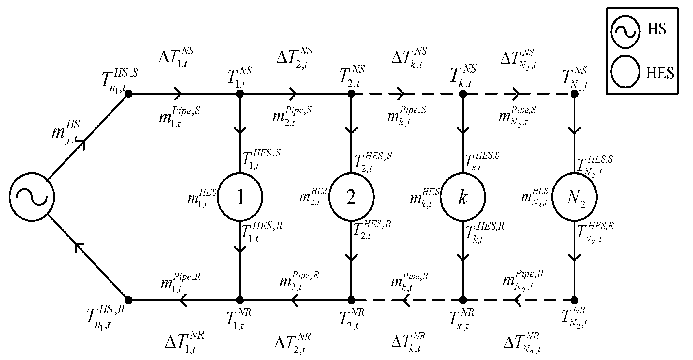
2.2. Model of DHS Considering a New Thermal Characteristic Index

The DHS consists of heat source (HS), pipeline network and heat load, and can usually be divided into heat transfer and distribution systems. The transmission system is usually radial, in which thermal energy is generated by the heat station, transferred by the circulating hot water flow driven by the circulating pump, and obtained by the heat exchanger station (HES) [26]. Heat is distributed from the secondary side of the heat exchange station to the end users in the distribution system. The transmission and distribution systems are indirectly connected through heat exchangers [27,28,29]. At present, most of the transmission DHS in northern part of China use the CF-VT control strategy. With this strategy, the temperature of the circulating water is adjusted to adapt to the changing heat load, while without changing the mass flow rate in the network. This strategy decouples the control of hydraulic conditions and thermal conditions in DHS, and has proven effective in industrial practice. In this paper, a new thermal characteristic index is proposed to measure the specific endothermic and exothermic capacity of DHN.

2.2.1. Heat Storage Characteristic of DHN

The DHN consists of a main network (long-distance heat transmission network) and an auxiliary network (distribution after the heat exchange substation). Figure 1 shows a main network based on the two-pipe direct return system. It allows one to control and maintain each terminal unit separately. Besides, the specific constraints of DHN are introduced in [20], such as heat loss, continuity of mass flow, temperature mixing and time delay. In this paper, quantized endothermic and exothermic level of DHN will be analyzed.
In order to balance the heat supply produced by HS and the heat demands needed by HES, DHN plays a regulating role as a heat storage device between HS and HES. When the HS produces excessive heat that cannot be consumed completely by HES, the extra heat is stored in DHN, which makes the average temperature of water flowing in DHN raised. On the contrary, considering energy saving and environmental protection, the HS produces heat, which cannot satisfy the heat demand of HES; the shortage heat is supplemented by DHN’s heat released, which makes the average temperature of water flowing in DHN drop down. Hence, the heat storage characteristic of DHN is achieved by the temperature change of water flowing in pipelines, briefly explained by Figure 1.
During time period t, the temperature drop of the return network in the pth pipeline node is shown as follows:
Δ T n , t N R = ( 1 + χ ) L c m p , t P i p e , R ( T n , t N R T t s u r f ) 2 π γ b ln ( d e x / d i n ) + 2 π γ b R e , p Γ P i p e , R , n N d p P i p e , R
where χ is the additional factor of heat loss caused by Appendix A, including valves and brace etcetera, T t s u r f is the temperature of soil surface at time t, γ b is thermal conductivity of insulation material and d i n is the internal diameter of pipe. If T n , t N R T t s u r f < 0, the value of Δ T n , t N R is negative, and it also means that the return pipelines will absorb heat due to the temperature difference between soil and the pipelines itself. The temperature drop of the supply network is by analogy. Furthermore, the expression of heat energy change of water flowing in supply and return pipelines can be obtained as follows:
Δ Q t N S = p Γ P i p e , S c m p , t N S Δ T n , t N S , n N d p P i p e , S
Δ Q t N R = p Γ P i p e , R c m p , t N R Δ T n , t N R , n N d p P i p e , R
As the value of Δ T n , t N R might be negative due to T n , t N R being lower than T t s u r f , the Δ Q t N S and Δ Q t N R need to be added together to gain the overall heat energy change caused by the temperature change of water flow in DHN.
Δ Q t D H N = Δ Q t N S + Δ Q t N R
where Δ Q t D H N denotes the endothermic or exothermic capacity of the water flowing in DHN. When the value of Δ Q t D H N is negative, indicating that the sum of CHP and EB heat generation is lower than heat load, and therefore the shortage heat energy is supplied by the internal energy of water flowing in DHN pipelines to compensate the heat energy difference between HS and HES. After that, the mean water temperature in DHN’s pipelines declines as a result of releasing energy. In contrast, when the value of Δ Q t D H N is positive it indicates that the sum of CHP and EB heat generation is higher than heat load, and hence the redundant heat energy is needed to be stored in water flowing in DHN’s pipelines. After that, the mean water temperature in DHN’s pipelines is raised as a result of absorbing energy. Like a heat storage tank, the DHN can own the endothermic and exothermic capacity by adjusting the water temperature. Therefore, the DHN can buffer heating supply and demand and improve the flexibility of CHP units without compromising the heating supply quality, which is further explained by a new heat characteristic index as follows:
To measure DHN’s heat regulation capability and the ability to maintain a stable indoor temperature, a new heat characteristic index TCI consisting of flexibility adjustment index (FI) and indoor temperature fluctuation index (TI) is proposed in this paper. FI should be maximized within the time frame considered, which is defined as follows:
F I = Δ Q t D H N Q t C H P , M a x
where FI represents the increased flexibility percentage of CHP heat output due to DHN, which is explained in Figure 2.
In Figure 2, the area ABCD represents the initial operation region of CHP units. After equipping EB devices, the equivalent power and heat output increase so that the feasible area expands to the area ABEC′D′. As DHN takes the role of heat storage device, the equivalent power and heat output increase so that the feasible area further expands to the area AA′B′E′C′D″. Seen from Figure 2, the red part area demonstrates that the DHN effectively improves the flexibility of the CHP unit’s output.
TI should be minimized within the operating cycle, which is defined as follows:
T I = b Γ H e a t   l o a d T b , t + 1 i n T b , t i n T b , 1 i n
where T b , 1 i n is the indoor temperature at an initial moment. When T b , t + 1 i n is close to T b , t i n , the fluctuation of indoor temperature is relatively stable. On the other hand, when the difference between T b , t + 1 i n and T b , t i n is large, it means that the indoor temperature fluctuates greatly, which will affect the comfort of human living. Thus, TI reflects the volatility rate of indoor temperature.
In general, the highest value of FI implies that DHN is the most beneficial for the flexibility regulation of CHP unit heat output. Moreover, the lowest value of TI implies the highest benefit in terms of indoor temperature stability. Therefore, to include the effects of the aforementioned indices in DHS, TCI is defined as follows:
T C I = ω 1 F I ω 2 T I
where the weighting factors 0 ≤ (ω1, ω2) ≤ 1, which ω1 + ω2 = 1, indicate the relative importance of each index for considering DHN. The choice of these factors mainly depends on the experiences and concerns of planners or decision makers. The equal weights are assumed for the proposed indices in this paper. In addition, TCI is used in the objective function of DHS in Section 3.1.

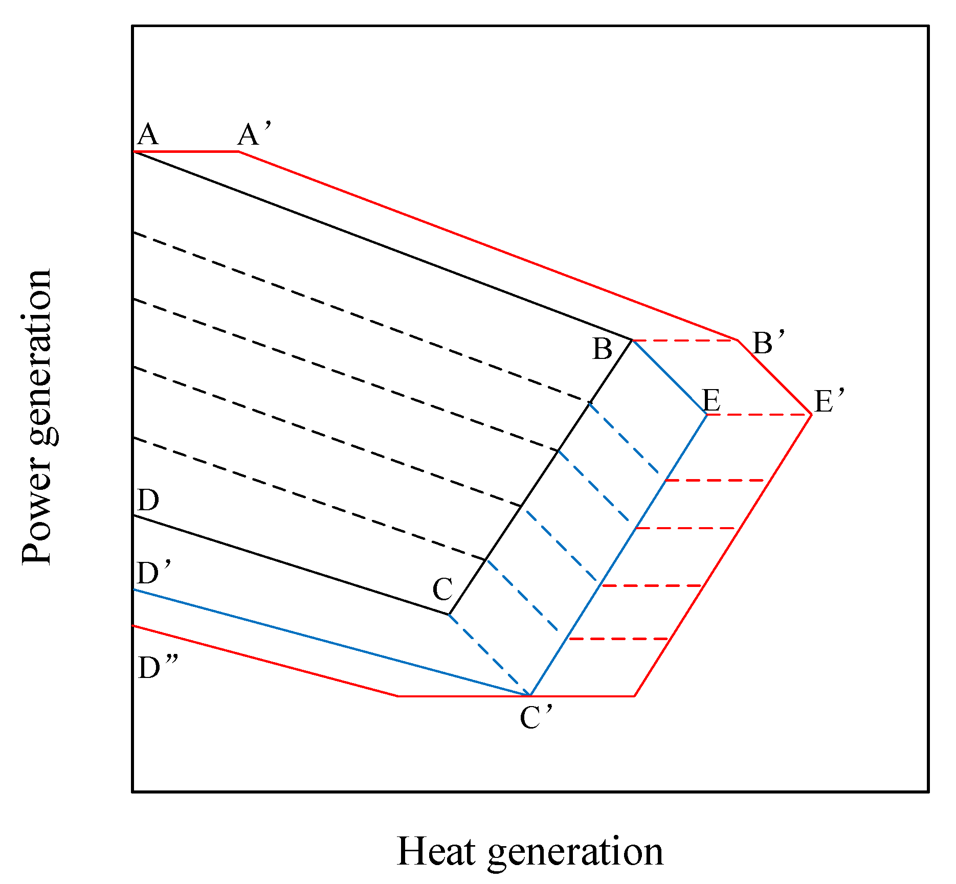
2.2.2. Relationship between K and TCI in TCES

In TCES, K can measure the reliability of EPS, and TCI can measure the flexibility of DHS. Although the two indexes measure different aspects of the system, they still have a link with each other due to the existence of thermoelectric sources such as CHP units. Besides, the function of DHN is like a heat storage device, and from Figure 2, it is seen that the power and heat adjustment range can be increased because of thermal storage device. Therefore, in this paper, the equivalent adjustment power range of CHP is as follows:
P t C H P , M i n P t E B T C I × Q t C H P , M a x × m u P t C H P + R t C H P P t C H P , M a x
From Equation (11), as the lower bound decreases, the overall adjustment range has increased. Furthermore, the regulating range of R t C H P is widened. Combining Equations (4) and (11), the probabilistic constraint is as follows:
P rob P t C H P , M a x ( P t C H P , M i n P t E B T C I × Q t C H P , M a x × m u ) P t C H P P t E L E ( P t E L ) K
Equation (12) is an uncertain probabilistic constraint, which can be converted into a linear form by using the method in Section 3.1. Therefore, the schematic relationship between K and TCI can be obtained in the following picture.
In Figure 3, line AB represents the threshold value of K towards different TCIs, and the region above line AB represents all possible values of K if sufficient spinning reserve capacity of CHP is equipped in this energy system. Besides, a0 + Δa…a0 + (n−1)Δa represents any interval within 0–1, and k0 + Δk…k0 + (n−1)Δk represents any probability interval within 0–100%, which will be determined by the specific configuration of the system. When TCI = 0, point A denotes the minimum reliability level of EPS. If K is still less than the value of A, it will no longer have research significance, as the reliability of the system could not be guaranteed. What is more, with the increase in TCI, the threshold value of K becomes larger, which means that the regulating flexibility of CHP become higher due to the consideration of DHN. However, this capacity is restricted by the operating parameters of each unit and DHN in the entire optimal scheduling. Thus, point B denotes the maximum value of TCI when the entire system parameters are determined, which means that DHN has reached its limit of flexibility regulation. Every different energy system has a different threshold line AB, so the actual line AB of each energy system is different. Point A, B and slope of the line are all different, depending on the operating parameters of each unit in the system, but K and TCI always maintain a positive correlation. In a word, in the following operation optimization, it is necessary to choose proper TCI and K toward the simulation system in order to obatin an optimal result.

3. Coordinated Operation Optimization

In order to improve the reliability and flexibility of the district energy system, the dispatch of EPS and DHS need to be combined and do a coordinated operation optimization. For EPS, the confidence level K is an important index to measure the reliability of a system, which means that with higher K, the reserve spinning capacity is more sufficient, and then the reliability of the system can be improved. For DHS, DHN plays a role similar to heat storage devices, which can significantly increase the regulating capacity of CHP units, and then the flexibility of the system can be enhanced. Thus, in this coordinated operation optimization model, in addition to reducing costs, enhancing the reliability and flexibility of system is necessary as well.

3.1. Objective Function

In this paper, the overall optimization objective for the whole district energy system is shown in Equation (13), which is composed of two parts, JEPS and JDHS. In EPS, JEPS consists of four parts, including the penalty cost of wind power curtailment, EES devices operation cost, fuel cost of CHP units, and spinning reserve cost. Besides, the first term is to prioritize the use of clean energy, the second term is to reduce the emission of pollutants, the third term is to decrease the operation cost of EES and the last term is to restrict the use of spinning reserve capacity. In DHS, JDHS is the compensation cost used to regulate the flexibility of system.
J = min ( J E P S ( P t w , P t E E S , α t k , R t C H P ) + J D H S ( Q t C H P , Q t E B , T n 1 , t H S , S , Δ T n , t N S , T j , t N S , T k , t H E S , S , T k , t H E S , R , T b , t i n , Δ T n , t N R , T j , t N R , T n 1 , t H S , R ) )
where the first term JEPS represents the weighted sum of the cost for the EPS, which is expressed as follows:
J E P S ( P t w , P t E E S , α t k , R t C H P ) = φ w t = 1 T ( P ¯ t w P t w ) + φ a × P t E E S , M a x + φ b × S O C t M a x + φ e × t = 1 T P t E E S + t = 1 T k = 1 M α t k c k + t = 1 T φ r R t C H P
where the first term φ w t = 1 T ( P ¯ t w P t w ) is the penalty cost of wind power spillage to make full use of wind power, φw is the penalty factor of wind curtailment of the wind turbine, and P ¯ t w is the predicted available wind energy of the wind turbine at time t; the second term φ a × P t E E S , M a x + φ b × S O C t M a x + φ e × t = 1 T P t E E S is EES device operation cost, φa and φb are the power-specific and energy-specific investment costs, respectively, P t E E S , M a x is the maximum output of EES devices at time t, S O C t M a x is the maximum storage capacity of EES at time t and φe is the operating cost factor; the third term t = 1 T k = 1 M α t k c k is the overall fuel cost of CHP unit, and the CHP model will be introduced in Section 3.2; the last term t = 1 T φ r R t C H P is the spinning reserve cost, and φr is the spinning reserve pricing.
The problem with DHS optimization is that it tries to find the minimum TI and maximum FI. When DHN is considered in DHS, with high flexible regulation applied in DHN, the temperature difference will change significantly, which makes an impact on the stability of indoor temperature fluctuations. Therefore, a new multi-objective index TCI should be maximized in coordinated optimal scheduling. As the highest TCI implies, the maximum benefit lies in considering DHN in terms of both heat regulation flexibility and temperature stability. However, the overall objective function is the minimum of the sum of costs of J E P S and J D H S ; J D H S should take the minimum costs. Therefore, J D H S = φ m t = 1 T M O I , which means that J D H S will obtain a more optimal result with higher TCI. Besides, φm is the price compensation factor. In a word, the function of J D H S means that if the DHN has a higher heat regulation capacity, higher incentive compensation costs will be produced in DHS, and then J D H S will obtain more minimum and optimal value.

3.2. Constraints

In this paper, CHP units are the main HS, which couples the electricity and thermal energy sectors and plays an important role in providing heat distribution and balancing intermittent wind power generation systems with high permeability [30]. Besides, when wind curtailment occurs, EB equipment will operate at maximum power to accommodate wind power generation, and the model of EB is introduced in [31]. In the heat station shown in Figure 1, the hot water from the DHN return pipe is heated by the heat generation of CHP and EB, and flows into the supply pipe again. The heat transfer from the thermal station to the water flow is described as follows:
Q t E B + Q t C H P = c × m j . t H S × ( T n 1 , t H S , S T n 1 , t H S , R ) , j Γ H S , n 1 N d j H S
Supply temperatures of heat sources should be kept above a threshold to guarantee the serving quality without exceeding its upper limits to prevent steam forming.
T ¯ n 1 , t H S , S / R T n 1 , t H S , S / R T ¯ n 1 , t H S , S / R , j Γ H S , n 1 N d j H S
For HESs, heat is transferred from the transmission network to the distribution network to provide sufficient heat to meet residential and commercial heating needs. Therefore, from the perspective of the transmission network, the heat exchange station is modeled as a heat load. The power of heat exchanger can be expressed as.
Q a , t H E S = c × m a . t H E S × ( T n 2 , t H E S , S T n 2 , t H E S , R ) , a Γ H E S , n 2 N d a P i p e
The return temperature of heat exchanger is required to exceed a threshold to ensure the load-serving quality and is lower than an upper limit to prevent steam forming.
T ¯ n 2 , t H E S , S / R T n 2 , t H E S , S / R T ¯ n 2 , t H E S , S / R , a Γ H E S , n 2 N d a H E S
In fact, the heat transfer process of the building envelope includes convection, conduction and radiation. Therefore, the steady-state heat loss is used here to simplify the calculation of some buildings where the indoor temperature is allowed to change at appropriate intervals. Equation (19) is the sum of three terms including heat conduction, heat convection and heat radiation [32].
Q b , t L o s s   = λ b A b T b , t i n T b , t o u t Δ d + h b A b ( T b , t o u t T b , t a m b )   + ε b β b A b ( 273.5 + T b , t o u t ) 4 , b Γ H e a t   l o a d
where λ b , h b , ε b and β b are factors of heat conduction, convection, radiation and correction, respectively.
The thermal mass in the building can decrease the peak heat load and the magnitude of indoor temperature fluctuations [33]. All of the heat acquisition and heat consumption of the bth heat load in the building during time period t can be expressed by the lumped heat source term Q a , t H E S .
Q b , t L o s s + c b m b ( T b , t + 1 i n T b , t i n Δ t )   = Q a , t H E S , a Γ H E S , b Γ H e a t   l o a d
where cb and mb are the specific heat capacity and mass flow of indoor air, respectively. To reflect the actual situation, the product of cb and cm can be obtained by an engineering experiment. In this TCES, there are power and heat equilibrium as follows:
For power equilibrium in EPS:
P t E E S + P t C H P = P t E B + E ( P t E L )
For heat equilibrium in DHS:
Q t C H P + 1 m u R t C H P + Q t E B = a Γ H E S Q a , t Δ t H E S + Δ Q t D H N
where mu is the ratio of power to heat under extraction mode. If there is no need for reserve capacity, R t C H P is set to zero.

3.3. Solving Method of Nonlinear Constraints

In this paper, Equation (4) is a nonlinear probabilistic constraint, which is used to ensure the reliability of EPS by adjusting confidence level K. Equations (5), (6), (15) and (17) are nonlinear constraints of DHS.
In this optimization model, because there are some essential nonlinear constraints in this TCES, it is necessary to transform overall non-linear model into a linear form.
Firstly, in order to transform the chance constraint expressed in Equation (4) into a deterministic form, we introduce a new type of 0–1 variable Z i c , t , which satisfies the following relationship.
R t C H P + E ( P t E L ) i c , t q ϖ Z i c , t 1 + R t C H P + E ( P t E L ) i c , t q ϖ , i c , t = 0 , 1 , , N c , t
where ϖ is a large positive number, ic,tq is discretized P t E L , which will be introduced in Appendix A in detail. When the inequality R t C H P i c , t q E ( P t E L ) holds, Equation (23) is equal to the inequality χ Z i c , t 1 + χ (where χ is a small positive number), and at the same time Z i c , t is a 0–1 variable. Thereby, this variable Z i c , t can only be driven to 1. In a similar way, if the inequality R t C H P i c , t q E ( P t E L ) holds, Equation (23) is equal to the inequality χ Z i c , t 1 χ , and hence Z i c , t can only be equal to 0 for the same cause. Therefore, Equation (4) is simplified as follows:
i c , t = 0 N c , t Z i c , t c ( i c , t ) κ
where c ( i c , t ) is a probabilistic sequence of P t E L , which will be introduced in Appendix A in detail. According to the above Equations, the EPS model based on chance constrained programming has been transformed into a readily MILP formulation.
Secondly, to transform constraints (5), (6), (15) and (17) into a linear form, the CF-VT control strategy is adopted in this paper. In this way, the mass flow rates anywhere are deemed as constants during the scheduling time period. Therefore, the constraints of DHS are converted into linear constraints.
Ultimately the energy system model joint of EPS and DHS can be solved by linear solver in Matlab software. The overall model solution process is as follows Table 1.

4. Case Study

The case study is conducted using a two-bus power system with wind and EES integration, where the CHPs and EB supply heat in a six-node DHN. Besides, CHP units and EB are all connected to Bus#2 in the power grid. The programs are developed using Matlab R2018b, and all MILPs are solved with the solvers of Yamip and Cplex. The one-line diagram of the test system is shown in Figure 4.
The heat load in the DHN is supplied by the heat station with two extraction-condensing CHP units and one EB device. The system configuration is shown in Table 2.
For EPS, the parameters of the WT are as follows: the installed capacity of the CHP unit is 100 MW, the installed capacity of EES is 15 MW and the installed capacity of EB is 80 MW. For DHN, as the temperature of the heat water flowing in pipelines is limited, the double-pipe supply/return pipeline system has taken in DHN. The mass flow rates of one pipeline network contained in the double-pipe supply/return pipeline system are as follows: m 3 . t H E S = 77.11 t/h = m 3 , t P i p e , S = m 3 , t P i p e , R , m 2 . t H E S = 89.94 t/h, m 2 , t P i p e , R = 167.05 t/h = m 2 , t P i p e , S , m 1 . t H E S = 94.17 t/h, m 1 , t P i p e , R = 261.22 t/h = m 1 , t P i p e , S = m j . t H S . Besides, both of the two networks have the same mass flow rates. The other parameters of DHN are as follows: γe = 2.4 W/m·°C, γr = 15 W/m2·°C, din = 2 m, dex = 2.114 m, χ = 0.1, γb = 0.023 W/m·°C, Re = 0.049 m·°C/W, Tin,Min = 20 °C, Tin,Max = 24 °C, and Tin,ch = 1 °C. Besides, Appendix B shows the profiles of total electric and heat load, as well as the forecast values and prediction intervals of available wind power.

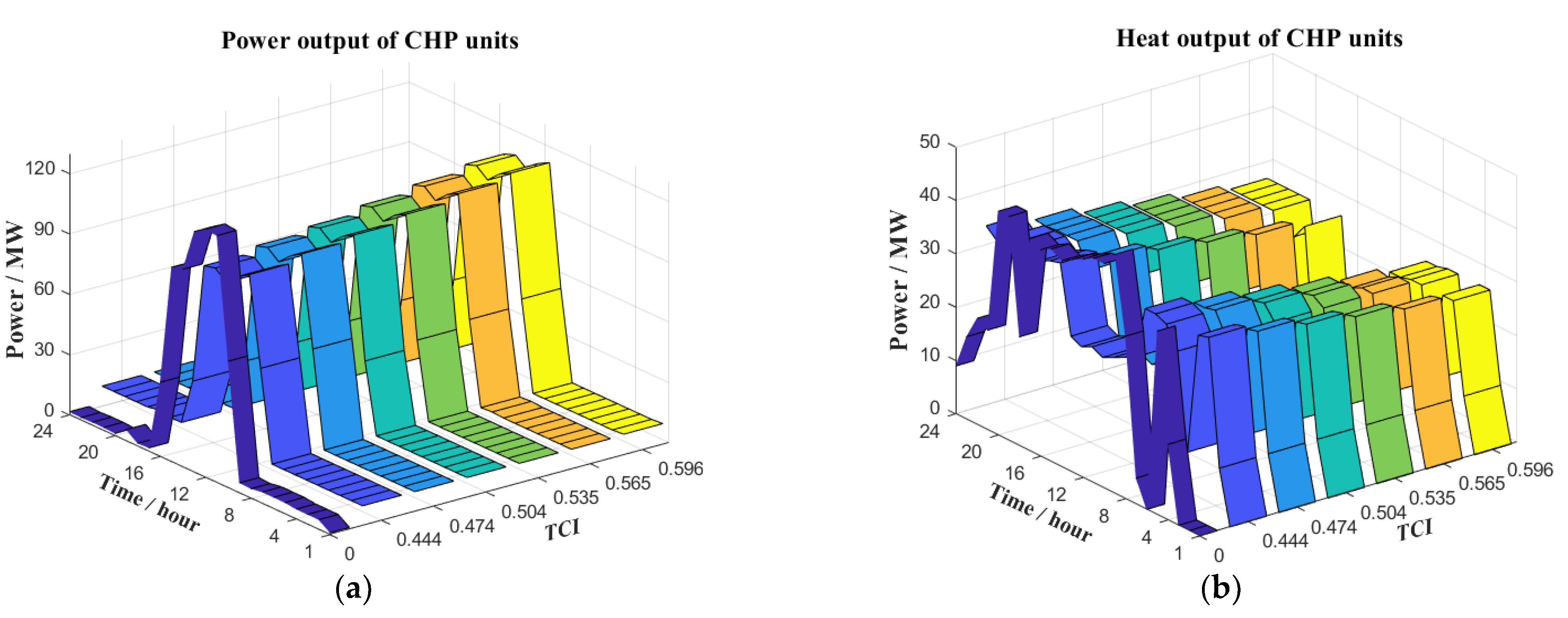
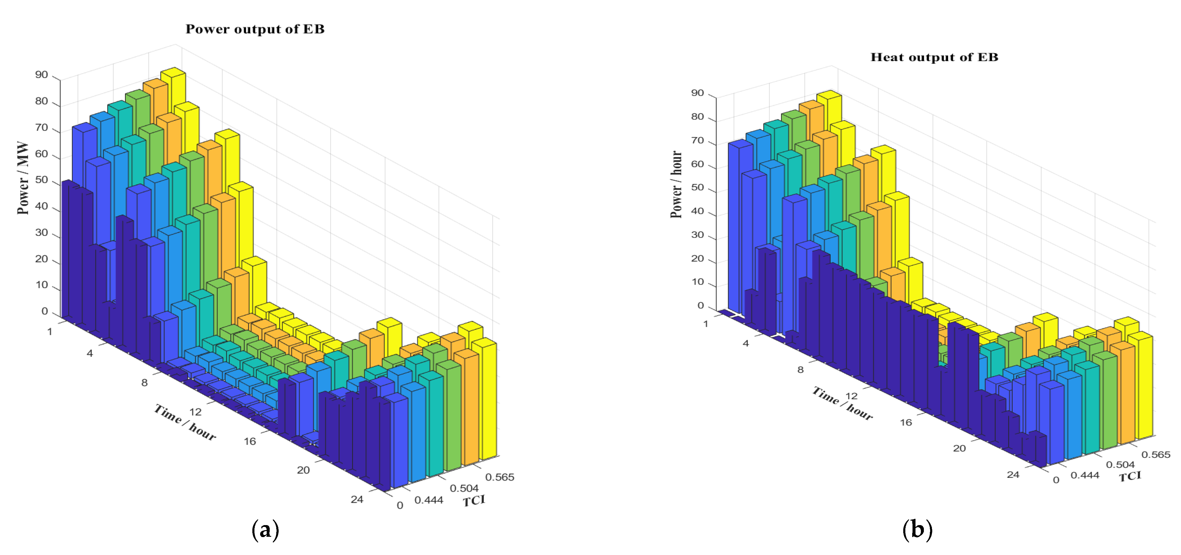
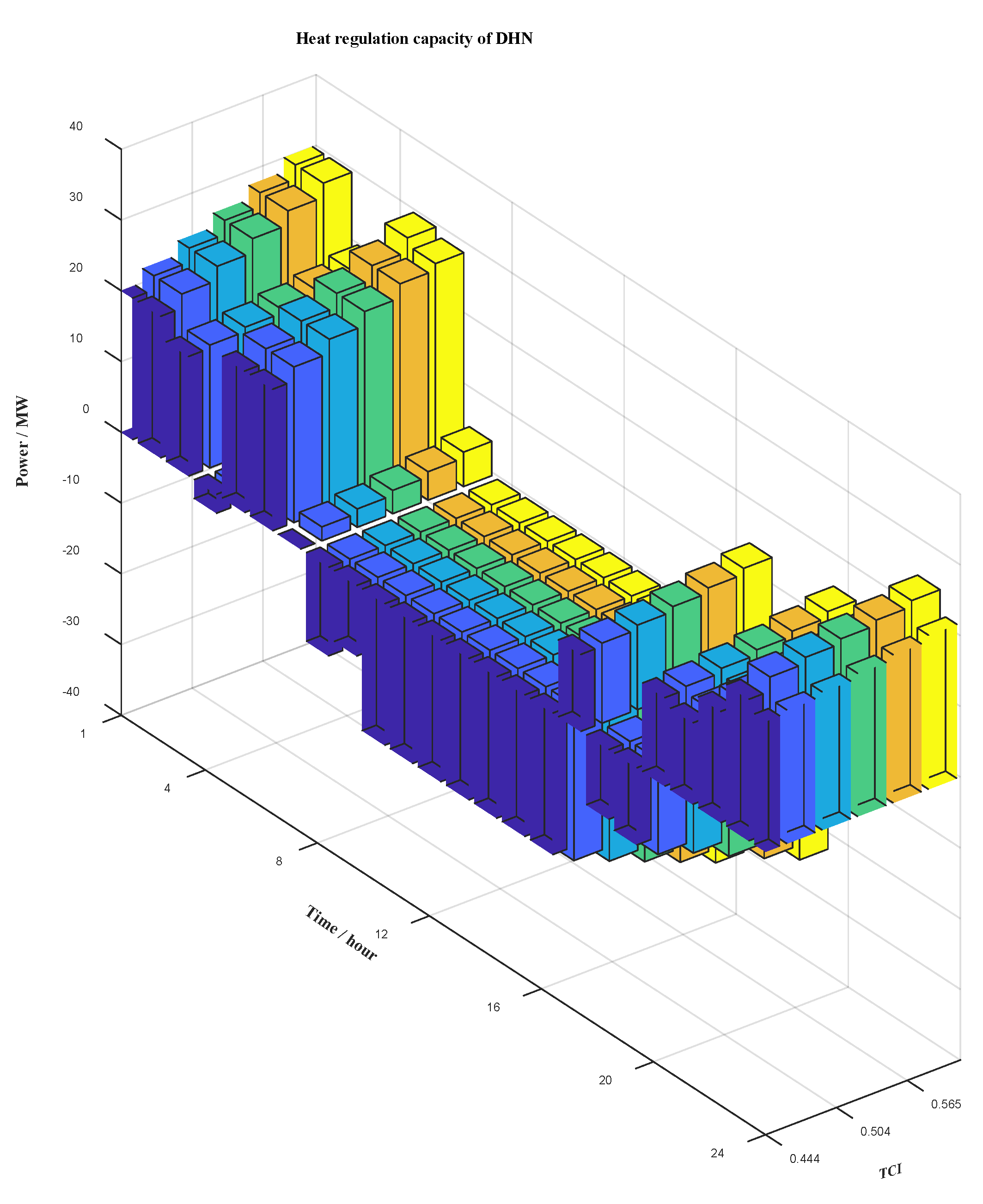
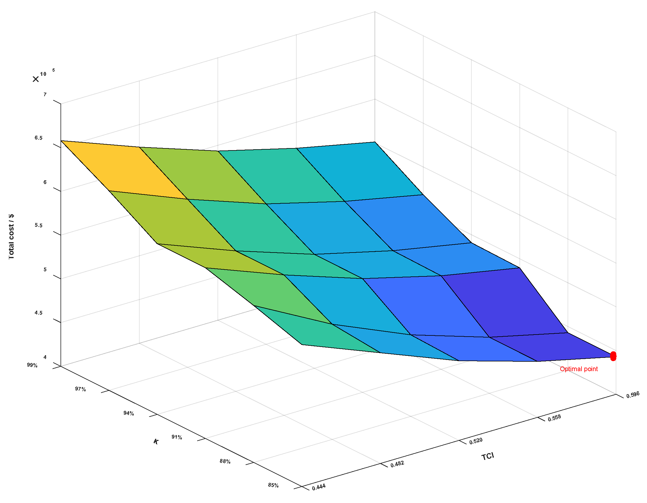
4.1. Comparative Tests with Different TCIs

To dominate the main effect of DHN, the test without considering DHN (TCI = 0) is used for comparison with the following simulation at the confidence level K = 85%. At this condition, the power and heat output results of CHP units and EB are shown in Figure 5 and Figure 6. Given the same confidence level K = 85% (85% is determined according to the configuration of this simulation system) over the scheduling period to guarantee the reliability of system, a set of comparative tests with a mean TCI value from 0 to 0.596 have been carried out, and, namely, the endothermic and exothermic capacity of DHN is from 0 to 30 MW. Besides, the calculation method of TCI is in Equations (11)–(15), and the maximum value 0.596 is determined according to parameters of DHN.
From the above figures, it can be concluded that when without considering the effect of DHN (TCI = 0), both the power and heat output of CHP units are higher than considering DHN, which will lead to higher fuel costs. Besides, with the increase in TCI, DHN will have a stronger heat regulation capacity, and the performance is that heat output of CHP will decline, although the power output of CHP increases slightly. For EB devices, without considering DHN, the heat output of EB will be higher, especially from time 8:00 to 16:00, due to a lack of a heat storage device such as DHN to regulate heat balance. Comparing the results of Figure 6a,b the most different point is that power output of CHP units increase with the increase in TCI, but the heat output of CHP units shows an opposite trend. Besides, when TCI = 0, both the power and heat output of CHP units reach maximum value. In Figure 6a,b, both the power and heat output of EB rise with the increase in TCI. In addition, when TCI = 0, especially in the time period from 8:00 to 16:00, the heat output of EB reaches maximum value, which means that it releases the previously stored heat.
In a word, due to the lack of DHN to regulate heat supply and demand, the heat generations by EB and CHP units need to adjust to ensure load demands. On the one hand, without considering DHN (TCI = 0), the increased output of CHP units will lead to higher fuel costs. On the other hand, the reduction in the power consumption of EB during the time period from 8:00 to 16:00 will cause a part of the curtailed wind energy not completely consumed by EB, which will also result in wind energy not being fully utilized ultimately. Excluding the time period from 8:00 to 16:00, the thermal output of EB is dominant, and CHP units play an auxiliary role to maintain heat equilibrium. TCI represents the capacity of heat release and store by DHN, and when TCI is higher, it means that DHN has high endothermic or exothermic capability. In other words, DHN can compensate the difference between heat source and load, and meanwhile the fuel cost of CHP is decreased due to lower heat output. If the value of TCI becomes higher than 0.595 in Figure 5b, some of the CHP units might be shut down, which will cause extra unit start and stop cost, so that TCI has an upper range limitation. To deeply analyze the quantized heat regulation level of DHN, with TCI from 0.444 to 0.596, the corresponding result is shown in Figure 7.
Figure 7 shows the specific heat regulation capacity and heat status of DHN at different TCIs. When the value of the bar is positive, it means that the heat released by supply pipelines is more than the heat stored in the return pipelines, so that the DHN plays a load role to absorb the extra heat produced by the heat source. Otherwise, when the value of the bar is negative, it indicates that the heat stored by return pipelines is more than the heat released in the supply pipelines, so that the DHN stores the extra heat from HES to reach the equilibrium between HS and HES. To sum up, the DHN has the same function with heat storage device, and the value of TCI could reflect the charge and discharge capacity of the DHN. At the 10:00–16:00 time period, the DHN might reach its maximum discharge capacity to satisfy load demand, which means that the DHN has fully exerted its nature. In a word, with higher TCI 0.596, DHN will have strong heat regulation capacity, which can improve the flexibility of a system correspondingly.

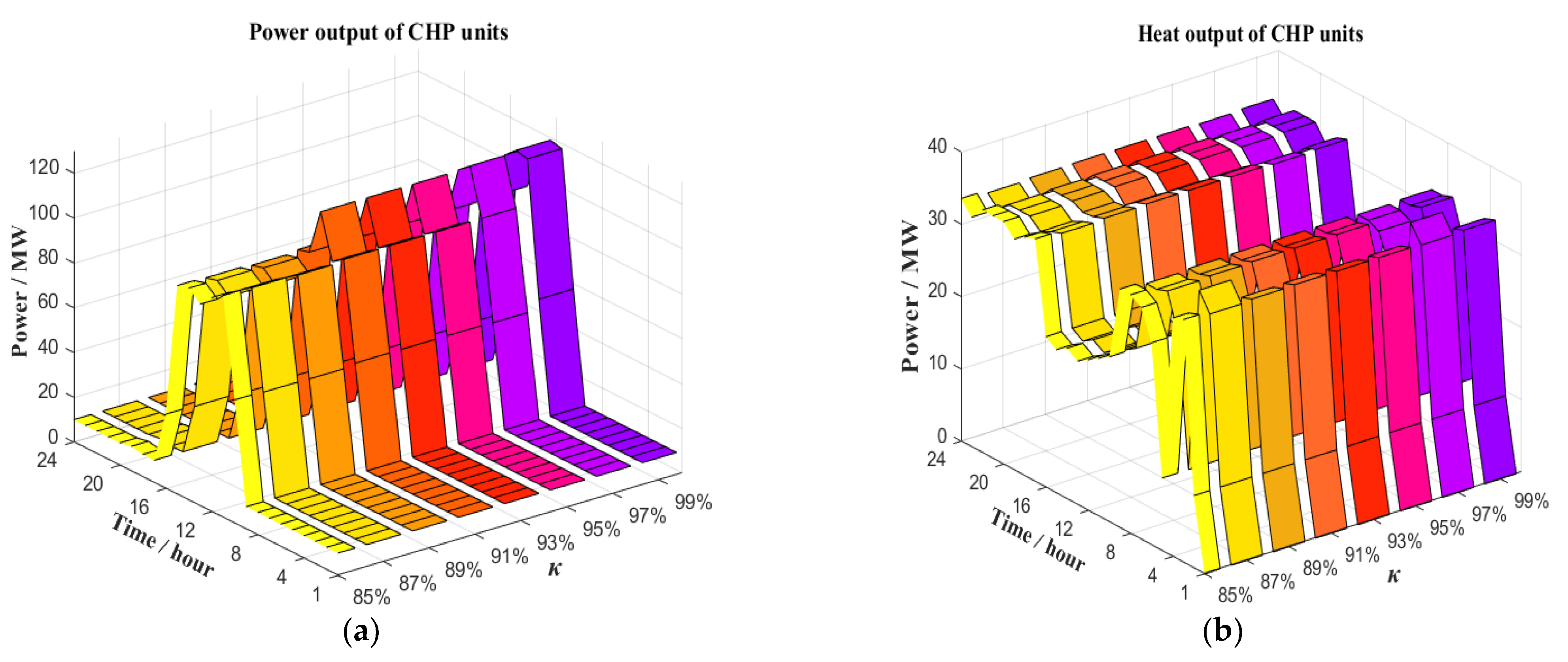
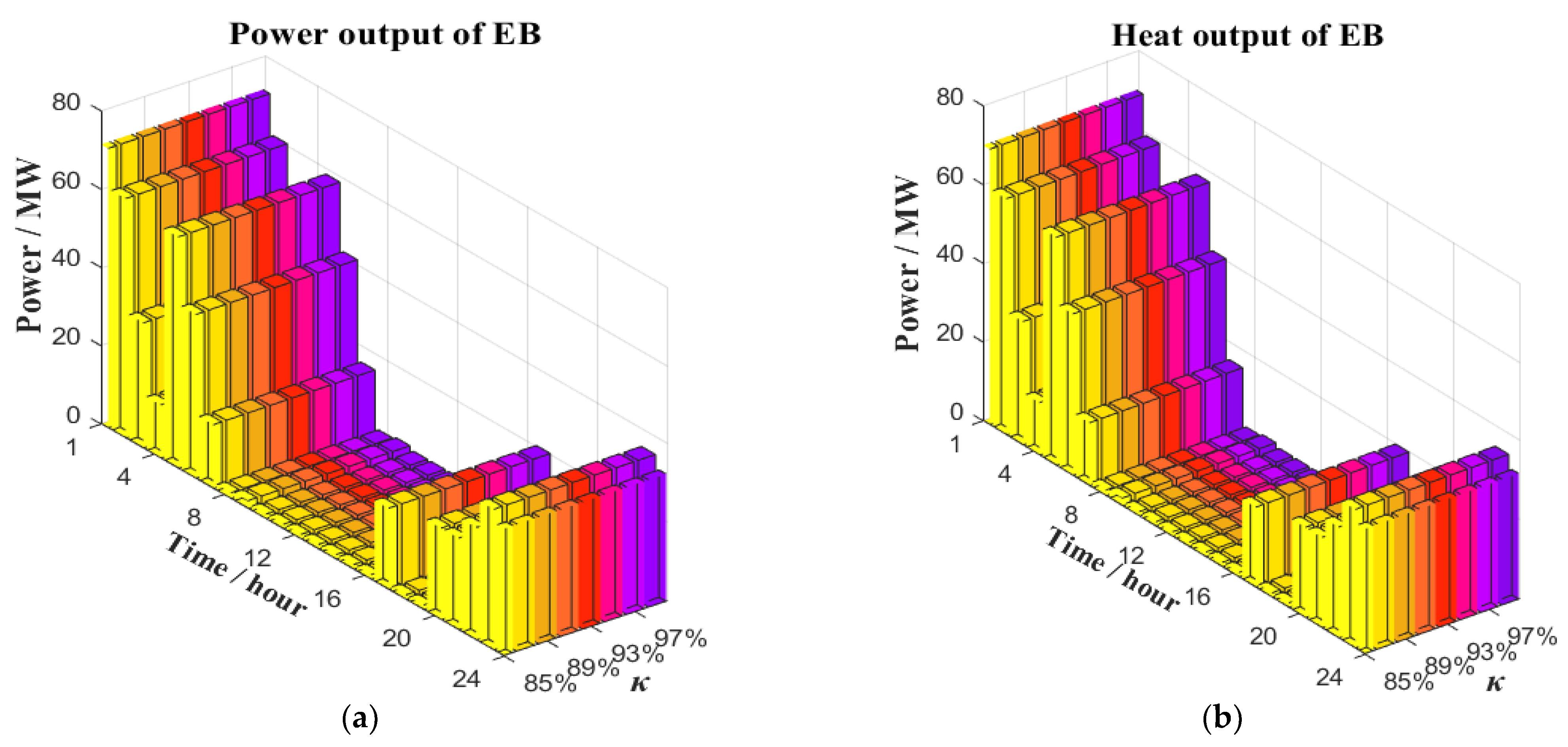
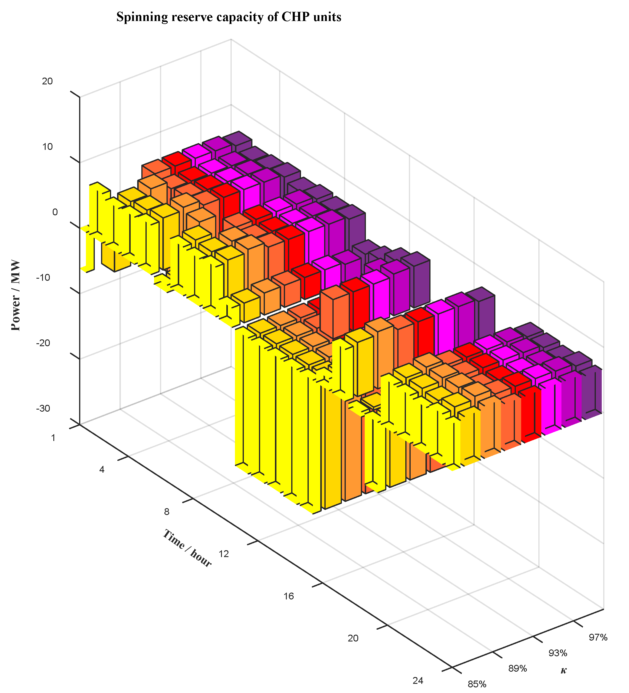
4.2. Comparative Tests with Different K

The minimum value of K = 85% from the above pictures is determined according to the installed capacity of all kinds of units in this simulation system. From Figure 8a,b, it can be seen that with the increase in K, the power output of CHP units starts to rise; otherwise, the heat output of CHP units still keeps stable. Besides, in Figure 9a,b, with the change of K, the change of both power and heat output of EB are not obvious. During the 8:00–16:00 time period, the power output of CHP is increasing. During the time periods 1:00–8:00 and 16:00–24:00, a large amount of curtailed wind energy is absorbed by the EB device. In addition, with the confidence level K enhanced, the power output curves of CHP units begin to change noticeably, and the maximum power output of CHP units can reach nearly 120 MW at K = 99%.
It can be concluded from the above figures that with higher K, the spinning reserve capacity of the CHP is used more fully to compensate for the uncertainty of WT and load, so the power output of CHP gradually starts to fluctuate to respond to the change of spinning reserve capacity. When K is from 85% to 99%, the corresponding spinning reserve capacity of CHP is shown in Figure 10.
To analyze the effect of K toward the spinning reserve capacity of CHP, the comparison of spinning reserves at different K is arranged, shown in Figure 10. It indicates that during the time period 11:00–15:00 and 20:00, more spinning reserve capacity needs to be prepared to maintain the required confidence level, which also shows that the difference between expected and actual values of P t E L is large at these time periods. Besides, when the rotating reserve value is negative, the power output of CHP could be declined.
Therefore, it can be inferred that when the higher K is requested, CHP with a large adjustment range of power output should be equipped. In order to increase the adjustment range of CHP, EB is the first option to be equipped with CHP in this paper, which can expand the negative direction output range of CHP. Besides, with higher K, facing the same uncertainty condition, CHP unit has sufficient capacity to compensate for fluctuation, which can ensure the reliability of system. What is more, when different TCIs and K are combined in simulation, different optimization costs will be generated. The result is shown in Figure 11.
As shown in Figure 11, with the increased confidence level K, the system needs to configure CHP units with more spinning reserve capacity, which inevitably increases the operating costs due to higher spinning reserve costs. In the opposite way, with the enhanced TCI, the system has to reduce the heat output of CHP units, which will lead to the decrease in fuel costs. In the above figure, it can be seen that total costs will decline with the increase in TCI and the decrease in K. Especially when K is 85% and TCI is 0.596, the total cost is lowest, which means that this system reaches an optimal result point. On the contrary, when K is 99% and TCI is 0.444, the total cost is highest. Therefore, it is substantial to select the appropriate confidence level K and TCI to make the system reach a better balance between reliability, flexibility and economy.

5. Conclusions

In this paper, a TCES scheduling model is proposed. For EPS, applying the high reserve capacity of CHP to offset the uncertainty of wind power and loads can improve the reliability of a system. Besides, in DHS, the quantized heat storage of DHN is utilized to regulate heat flow between HS and HES, which is measured by a new proposed thermal characteristic index. In the joint model solve process, some non-linear constraints are converted to a linear form by discretized step transformation and the CF-VT control strategy. Case studies demonstrate that the overall costs increase as the confidence level of EPS rises, and conversely the total costs rise with the TCI of DHS declining. The optimal result of tests can reach the balance of reliability, flexibility and economy of the district energy system.

Author Contributions

Investigation, Q.T.; Writing—original draft, G.L.; Writing—review & editing, B.H. and M.M. All authors have read and agreed to the published version of the manuscript.

Funding

This research was funded in part by the State Key Laboratory of Alternate Electrical Power System with Renewable Energy Sources grant number LAPS21007, in part by Guangdong Basic and Applied Basic Research Foundation grant number 2021A1515110778, in part by the Fundamental Research Funds for the Central Universities grant number N2104014.

Institutional Review Board Statement

Not applicable.

Informed Consent Statement

Not applicable.

Conflicts of Interest

The authors declare no conflict of interest.

Nomenclature

AbbreviationswWind Turbine
CHPCombined heat and powerkCorner point of CHP operation region
DHNDistrict heating networkHS,SHeat resource on the supply side
EPSElectric power systemHS,RHeat resource on the return side
DHSDistrict heating systemHES,SHeat exchange station on the supply side
TCESThermoelectric coupling energy systemHES,RHeat exchange station on the return side
CF-VTConstant mass flow and variables temperatureinIndoor temperature
TCIThermal characteristic index outOutdoor temperature
EESElectric energy storageNSNode in supply pipeline
EBElectric boilerNRNode in return pipeline
WTWind turbinesurfSoil surface
HESHeat exchange stationPipe,SSupply pipelines
HSHeat resourcePipe,RReturn pipelines
ELEquivalent loadsurfSoil surface
Greek lettersSubscript
KConfidence leveltTime moment s
βElectrothermal conversion efficiencyn1Node of HS
ΓIndex set of pipes in the DHNn2Node of HES
λFactors of heat conductionbBuilding envelope
εFactors of heat radiationRoman letters
νVelocity of water flowPPower output MW
γCoefficient of heat transformation QHeat output MW
μAdditional factor of heat lossRPower reserve capacity MW
φPenalty factorSTOperating status of EB
ωWeighting factor of DHNTTemperature ℃
ΨWeight coefficientmMass flow t/h
χSmall positive numberRampRamp rate of CHP
ϖ Large positive numberJObjective function
SuperscriptsEExpectation value of EL MW
LPower load injectionsZ0–1 variable

Appendix A

Appendix A.1. Serialization Modeling of Random Variables in EPS

During the time period t, the WT output Pw and the load power PL are random variables, and they can be described by the corresponding probability sequences a(ia,t) and b(ib,t) by discretizing the continuous probability distribution. The length calculation formulas of the WT output and load power probability sequence Na,t and Nb,t are as follows:
N a , t = [ P t w , M a x q ] , N b , t = [ P t L , M a x q ]
where q denotes the discrete step size. P t w , M a x and P t L , M a x are the maximum value of wind and load power at time t.
The probability sequence output by WT can be calculated by using its PDF, which is given as follows:
a i a , t = 0 q / 2 f w P w d P w , i a , t = 0 i a , t q q / 2 i a , q q + q / 2 f w P w d P w , i a , t > 0 , i a , t N a , t i a , t , q q / 2 i a , t q f w P w d P w , i a , t N a , t
The b(ib,t) can be obtained by analogy.
Given the length N c , t of probabilistic sequence P t E L , the probabilistic sequence of EL power c(ic,t) is calculated by the subtraction-type-convolution (STC) operation.
c ( i c , t ) = b ( i b , t ) θ a ( i a , t ) = i b , t i a , t = i c , t b ( i b , t ) a ( i a , t ) , 1 i c , t N c , t = [ P t E L , M a x q ] i b , t i a , t b ( i b , t ) a ( i a , t ) , i c , t = 0
Table A1 shows the correspondence between the probability sequence of the EL power PEL with the step size q and the length Nc,t.
Table A1. Probabilistic sequence of equivalent power.
Power(MW)0qic,tqNc,tq
Probabilityc(0)c(1)c(ic,t)c(Nc,t)
Table A1 shows that for a given EL power ic,tq, there is always a corresponding probability c(ic,t).

Appendix B

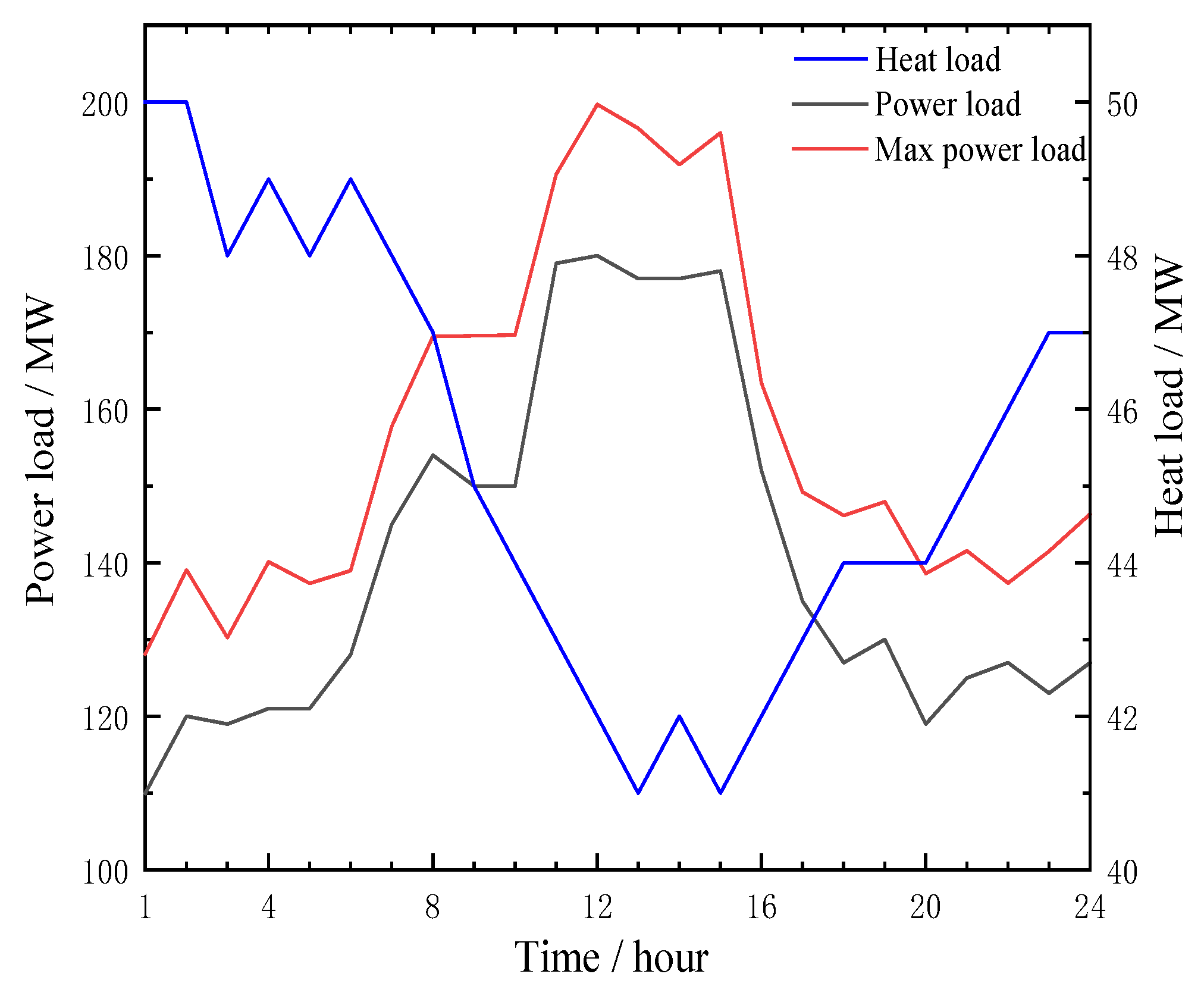
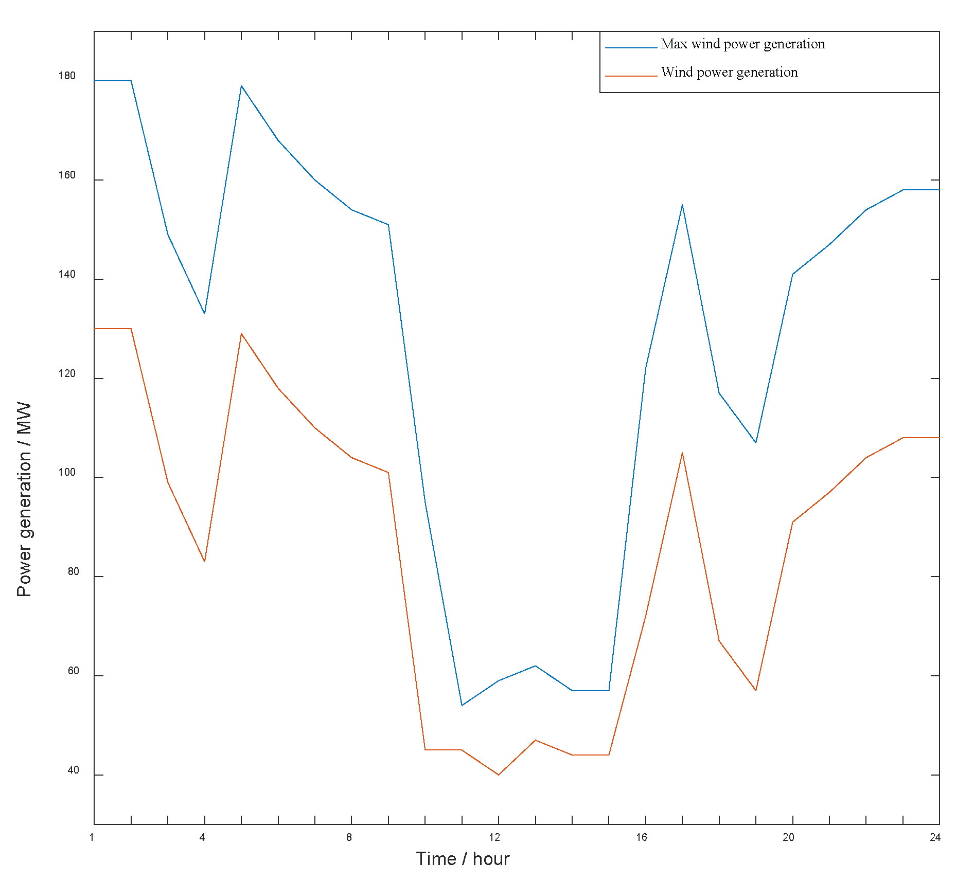
Appendix B.1. Profiles of Electric and Heat Load and Wind Power Forecast

Figure A1 shows the profiles of total electric and heat load, and the forecast values and prediction intervals of available wind power is shown in Figure A2. Compared to electrical loads, thermal loads have opposite peaks because thermal loads are negatively related to ambient temperature, while electrical loads are positively related to consumer activity. The hourly operation scheduling over 24 h is considered for the cases in this paper.
Figure A1. Profiles of electric and heat loads.
Sustainability 14 09764 g0a1
Figure A2. Profiles of wind power forecast.
Sustainability 14 09764 g0a2

References

  1. Xia, S.; Bu, S.Q.; Luo, X.; Chan, K.W.; Lu, X. An autonomous real-time charging strategy for plug-in electric vehicles to regulate frequency of distribution system with fluctuating wind generation. IEEE Trans. Sustain. Energy 2018, 9, 511–524. [Google Scholar] [CrossRef]
  2. Salomón, M.; Savola, T.; Martin, A. Small-scale biomass CHP plants in Sweden and Finland. Renew. Sustain. Energy Rev. 2011, 15, 4451–4465. [Google Scholar] [CrossRef]
  3. Barco-Burgos, J.; Bruno, J.C.; Eicker, U.; Saldana-Robles, A.L.; Alcantar-Camarena, V. Review on the integration of high-temperature heat pumps in district heating and cooling networks. Energy 2022, 239, 122378. [Google Scholar] [CrossRef]
  4. Wang, H.; Lahdelma, R.; Wang, X.; Jiao, W.; Zhu, C.; Zou, P. Analysis of the location for peak heating in CHP based combined district heating systems. Appl. Therm. Eng. 2015, 87, 402–411. [Google Scholar] [CrossRef]
  5. Li, X.; Li, W.; Zhang, R.; Jiang, T.; Chen, H.; Li, G. Collaborative scheduling and flexibility assessment of integrated electricity and district heating systems utilizing thermal inertia of district heating network and aggregated buildings. Appl. Energy 2020, 258, 114021. [Google Scholar] [CrossRef]
  6. Dou, C.; Yue, D.; Li, X.; Xue, Y. MAS-based management and control strategies for integrated hybrid energy system. IEEE Trans. Ind. Inf. 2016, 12, 1332–1349. [Google Scholar] [CrossRef]
  7. Yue, D.; Han, Q.L.; Lam, J. Network-based robust H∞ control of systems with uncertainty. Automatica 2005, 41, 999–1007. [Google Scholar] [CrossRef]
  8. Weng, S.; Yue, D.; Dou, C.; Shi, J.; Huang, C. Distributed event-triggered cooperative control for frequency and voltage stability and power sharing in isolated inverter-based microgrid. IEEE Trans. Cybern. 2019, 49, 1427–1439. [Google Scholar] [CrossRef] [PubMed]
  9. Li, Y.; Yang, Z.; Li, G.; Zhao, D.; Tian, W. Optimal scheduling of an isolated microgrid with battery storage considering load and renewable generation uncertainties. IEEE Trans. Ind. Electron. 2019, 66, 1565–1575. [Google Scholar] [CrossRef] [Green Version]
  10. Wen, S.; Lan, H.; Fu, Q.; Yu, D.C.; Zhang, L. Economic allocation for energy storage system considering wind power distribution. IEEE Trans. Power Syst. 2015, 30, 644–652. [Google Scholar] [CrossRef]
  11. Barani, M.; Aghaei, J.; Akbari, M.A.; Niknam, T.; Farahmand, H.; Korpas, M. Optimal partitioning of smart distribution systems into supply-sufficient microgrids. IEEE Trans. Smart Grid 2019, 10, 2523–2533. [Google Scholar] [CrossRef]
  12. Nasrolahpour, E.; Kazempour, J.; Zareipour, H.; Rosehart, W.D. Impacts of ramping inflexibility of conventional generators on strategic operation of energy storage facilities. IEEE Trans. Smart Grid 2018, 9, 1334–1344. [Google Scholar] [CrossRef] [Green Version]
  13. Wang, L.F.; Singh, C.N. Stochastic combined heat and power dispatch based on multi objective particle swarm optimization. Int. J. Electr. Power Energy Syst. 2008, 30, 226–234. [Google Scholar] [CrossRef]
  14. Piperagkas, G.; Anastasiadis, A.; Hatziargyriou, N. Stochastic PSO-based heat and power dispatch under environmental constraints incorporating CHP and wind power units. Electr. Power Syst. Res. 2011, 81, 209–218. [Google Scholar] [CrossRef]
  15. Chen, X.; Kang, C.; O’Malley, M.; Qing, X.; Bai, J.; Liu, C.; Sun, R.; Wang, W.; Li, H. Increasing the flexibility of combined heat and power for wind power integration in China: Modeling and implications. IEEE Trans. Power Syst. 2015, 30, 1848–1857. [Google Scholar] [CrossRef]
  16. Chen, L.; Liu, N.; Li, C.; Wu, L.; Chen, Y. Multi-party stochastic energy scheduling for industrial integrated energy systems considering thermal delay and thermoelectric coupling. Appl. Energy 2021, 304, 117882. [Google Scholar] [CrossRef]
  17. Liao, T.; Xu, Q.; Dai, Y.; Cheng, C.; He, Q.; Ni, M. Radiative cooling-assisted thermoelectric refrigeration and power systems: Coupling properties and parametric optimization. Energy 2022, 242, 122546. [Google Scholar] [CrossRef]
  18. Li, Z.; Wu, W.; Wang, J.; Zhang, B.; Zheng, T. Transmission-constrained unit commitment considering combined electricity and district heating networks. IEEE Trans. Sustain. Energy 2016, 7, 480–492. [Google Scholar] [CrossRef]
  19. Huang, J.; Li, Z.; Wu, Q.H. Coordinated dispatch of electric power and district heating networks: A decentralized solution using optimality condition decomposition. Appl. Energy 2017, 206, 1508–1522. [Google Scholar] [CrossRef]
  20. Zhang, T.; Li, Z.; Wu, Q.H.; Zhou, X. Decentralized state estimation of combined heat and power systems using the asynchronous alternating direction method of multipliers. Appl. Energy 2019, 248, 600–613. [Google Scholar] [CrossRef]
  21. Wu, C.; Gu, W.; Jiang, P.; Li, Z.; Cai, H.; Li, B. Combined economic dispatch considering the time-delay of district heating network and multi-regional indoor temperature control. IEEE Trans. Sustain. Energy 2018, 9, 118–127. [Google Scholar] [CrossRef]
  22. Merlin, K.; Delaunay, D.; Soto, J.; Traonvouez, L. Heat transfer enhancement in latent heat thermal storage systems: Comparative study of different solutions and thermal contact investigation between the exchanger and the PCM. Appl. Energy 2016, 166, 107–116. [Google Scholar] [CrossRef]
  23. Arefifar, S.A.; Mohamed, Y.A.R.I. DG mix, reactive sources and energy storage units for optimizing microgrid reliability and supply security. IEEE Trans. Smart Grid 2014, 5, 1835–1844. [Google Scholar] [CrossRef]
  24. Kalkhambkar, V.; Kumar, R.; Bhakar, R. Joint optimal allocation methodology for renewable distributed generation and energy storage for economic benefits. IET Renew. Power Gener. 2016, 10, 1422–1429. [Google Scholar] [CrossRef]
  25. Li, Z.M.; Aminifar, F.; Alabdulwahab, A.; Al-Turki, Y. Networked microgrids for enhancing the power system resilience. Proc. IEEE 2017, 105, 1289–1310. [Google Scholar] [CrossRef]
  26. Turski, M.; Sekret, R. Buildings and a district heating network as thermal energy storages in the district heating system. Energy Build 2018, 179, 49–56. [Google Scholar] [CrossRef]
  27. Dainese, C.; Faè, M.; Gambarotta, A.; Morini, M.; Premoli, M.; Randazzo, G.; Rossi, M.; Rovati, M.; Saletti, C. Development and application of a predictive controller to a mini district heating network fed by a biomass boiler. Energy Procedia 2019, 159, 48–53. [Google Scholar] [CrossRef]
  28. Robert, E.; Kalehbasti, P.; Michael, D. A novel approach to district heating and cooling network design based on life cycle cost optimization. Energy 2020, 194, 116837. [Google Scholar]
  29. Schwarz, M.B.; Mabrouk, M.T.; Silva, C.S.; Haurant, P.; Lacarrière, B. Modified finite volumes method for the simulation of dynamic district heating networks. Energy 2019, 182, 954–964. [Google Scholar] [CrossRef]
  30. Liu, L.; Zhu, T.; Pan, Y. Multiple energy complementation based on distributed energy systems—Case study of Chongming county, China. Appl. Energy 2016, 192, 329–336. [Google Scholar] [CrossRef]
  31. Lahdelma, R.; Hakonen, H. An efficient linear programming algorithm for combined heat and power production. Eur. J. Oper. Res. 2003, 148, 141–151. [Google Scholar] [CrossRef]
  32. Lbrahim, R.A. Overview of mechanics of pipes conveying fluids—Part I: Fundamental studies. J. Press. Vessel Technol. 2010, 132, 034001. [Google Scholar] [CrossRef]
  33. Zhou, J.; Zhang, G.; Lin, Y.; Li, Y. Coupling of thermal mass and natural ventilation in buildings. Energy Build 2007, 40, 979–986. [Google Scholar] [CrossRef]
Figure 1. Structure of the main network of DHN.
Sustainability 14 09764 g001
Figure 2. Schematic diagram of CHP expanded feasible region.
Sustainability 14 09764 g002
Figure 3. Schematic diagram of the relationship between K and TCI.
Sustainability 14 09764 g003
Figure 4. Diagram of two-bus power system with six-node DHN.
Sustainability 14 09764 g004
Figure 5. (a) Power output of CHP units. (b) Heat output of CHP units.
Sustainability 14 09764 g005
Figure 6. (a) Power output of EB. (b) Heat output of EB.
Sustainability 14 09764 g006
Figure 7. Heat regulation capacity under different TCIs.
Sustainability 14 09764 g007
Figure 8. (a) Power output of CHP units. (b) Heat output of CHP units.
Sustainability 14 09764 g008
Figure 9. (a) Power output of EB. (b) Heat output of EB.
Sustainability 14 09764 g009
Figure 10. Spinning reserve capacities under different confidence levels.
Sustainability 14 09764 g010
Figure 11. Effects of different confidence levels and TCI on the optimal results.
Sustainability 14 09764 g011
Table 1. The overall model solution process.
1:Model building:
2: Uncertainty model of EPS;
3: CF-VT modelling of DHN.
4:Model conversion:
5: Transform chance probability into deterministic MILP constraints;
6: Set the mass flow rates, and calculate the temperature of HS, HES, pipelines.
7:Model solving:
8: Enter the parameters of TCES;
9: Set the constraints and objective function;
10: Solve the model using Yamip and Cplex solvers;
11:  If find a solution?
12:  Output the optimal scheduling scheme;
13:  Else if
14:  Update K and TCI and return to Step 9.
15:End
Table 2. Configuration of test system.
Test SystemElectric Power SystemDistrict Heating Network
BusLineCHPWTEESEBNodePipelineHES
Number2221116103
Publisher’s Note: MDPI stays neutral with regard to jurisdictional claims in published maps and institutional affiliations.

