Abstract
The large-scale integration of renewable energy sources (RESs) has become one of the most challenging topics in smart grids. Indeed, such an integration has been causing significant grid stability issues (voltage and frequency control) due to the dependency of RESs on meteorological conditions. To this end, their integration must be accompanied by alternative sources of energy to attenuate the power fluctuations. Energy storage systems (ESSs) can provide such flexibility by mitigating local peaks/drops in load demands/renewable power generation. Therefore, the development of energy management strategies (EMSs) has been attracting considerable attention in the management of the power generated from the RESs associated with that which is stored/provided by the ESSs. Then, the optimization of the EMS leads to substantial savings in operation and maintenance and to correct decisions for the future. This study presents an optimized EMS for a wind farm, coupled with a pumped hydro energy system (PHES). The proposed day-ahead EMS consists of two stages, namely the forecasting and the optimization stages. The forecasting module is responsible for predicting the wind power generation and load demand. A random forest (RF) method is used to perform the power forecasting after the extraction of the weather data features using a kernel principal component analysis (KPCA) technique. Then, a nonlinear programming (NLP)-based optimization technique is proposed to define the day-ahead optimal energy of the PHES. The purpose of the optimization is to maximize the profit cost in a day-ahead horizon, taking into consideration the system constraints.
1. Introduction
The large-scale integration of RESs (photovoltaic and wind energy) into the power grid has grown rapidly in recent years. However, the intermittent nature of RESs poses some challenges to the continued expansion of their use [1]. Indeed, as the power production needs to be balanced with the power consumption, there is a requirement for reserve power capacities to ensure system reliability [2]. Energy storage systems (ESSs) can store energy when there is an excess energy during periods with low demand. Conversely, the ESS injects the stored energy when needed during peak load periods. As a result, the effect of the renewable power fluctuation can be reduced, and the rate of the RES integration can be increased. There are different types of energy storage used in power systems, such as flywheels, batteries, ultra-capacitors, and pumped hydro energy storage (PHES). The selection of the appropriate ESS usually depends on the application and power required. In the case of high-level RES penetration, the PHES and the compressed air energy storage (CAES) are considered to be the most promising storage systems. In [3], an EMS for grid-connected wind power generation coupled with PHES is proposed. Several studies have addressed the day-ahead EMS. The EMS is based on an algorithm that manages the power flow between the RES, the ESS, the load, and the grid to reduce the effect of the renewable power fluctuation. At first, the forecasted power generation will be fed to the EMS algorithm as input. Different studies have investigated the RE power forecasting. The study in [4] used machine learning methods (ML) for short-term wind power prediction. A hybrid learning model of two techniques (support vector regression (SVR) and multiple linear regression (MLR) was proposed. It has been concluded that SVR and SVR-based hybrid learning models offer better performance and generalization compared to multiple linear regression (MLR). The work in [5] claimed an improvement of wind power prediction from meteorological conditions using a decision tree (DT) method. The DT model was trained for four wind vertical profiles. The results indicate that when compared to traditional power curve methods, the DT improves prediction accuracy by 22% for the given data. In [6], the authors developed a heterogeneous ensemble between ML techniques (DT, k-nearest neighbors and SVR), which made use of multiple base algorithms and benefited from a gain of diversity among the weak predictors. In addition, a comparative study of machine learning techniques (extra trees, RF, ridge regression, DT, gradient boosting, the least absolute shrinkage and selection operator, and the convolutional neural network) was proposed for wind power prediction in [7].
For optimal power forecasting, many studies have dealt with pre-processing data using feature extraction and selection. The studies in [8,9] proposed the feature extraction of photovoltaic (PV) data, which aims to optimally detect faults in PV systems with RF, where the latter is preceded by the preparation of data inputs using feature extraction and selection (FES). While the purpose of the feature extraction is to distinguish the characteristics that accurately/better describe the system operation, feature selection seeks to pick a small subset of features based on certain criteria. In the literature, principal component analysis (PCA) [10], independent component analysis (ICA) [11], and partial least squares (PLS) [12] have been the most applied feature extraction techniques. A comparison of PCA, KPCA, and ICA for dimensionality reduction in a support vector machine was presented in [13]. In [14], the authors proposed a KPCA-based approach for renewable energy forecasting for the nonlinear characteristics extraction of the high-dimensional feature. Moreover, the research in [15] proposed a survey on deep learning (DL)-based wind power forecasting. The latter paper provided a comprehensive review on DL, reinforcement learning, transfer learning, recurrent neural network (RNN), deep belief network (DBN), deep neural network (DNN), and other techniques for wind speed and wind power forecasting modeling. The presented results showed that a hybrid method based on DL can effectively combine the advantages of different methods and can effectively improve the prediction accuracy of wind power.
The optimal forecasting model represents the most important component in EMS optimization. Different studies have proposed day-ahead EMS. In [16], the authors discussed the optimum schedule of the joint/uncoordinated operations of the PHES-based wind farms in the electricity market. The scheduling problem was modeled as a stochastic problem optimization. The presented results show that the profit is increased with joint operation in comparison with the uncoordinated operation. The study in [17] dealt with the optimization scheduling of system composed of a PV system and PHES. The maximum profit was fixed as the problem objective. The results indicate that the pumped storage can effectively increase the power benefits and access capacity of PV and wind power. In [18], the authors studied the effect of using PHES combined with local grid strengthening for smooth wind power generation. For a maximized wind power capacity, scheduling methods have been proposed based on a multi-objective optimization procedure. As objective functions, wind energy reduction costs, total social costs, and energy from PHES units are considered. In [19], a day-ahead optimal scheduling model of a hybrid power system (wind/thermal) using PHES was studied, where a particle swarm optimization algorithm was used. The objective of the optimization problem was to reduce the production costs and the devastating carbon emissions. The work in [20] investigated the combination between a wind farm and a PHES. Stochastic coding has been considered as a decision-making procedure. A dynamic planning technique was proposed by [21] for building optimal wind power management to decrease the discrepancy between the production power and the load demand. The authors in [22] investigated the coupling of a wind farm with a PHES. The PHES was used to achieve high economic gain from wind energy systems with intermittent characteristics. In addition, a linear programming method was used for the optimization of the EMS.
All the previous studies have only focused on the energy management from the optimization perspective. However, the current paper proposes a two-stage EMS for a wind farm coupled with a PHES, using advanced forecasting and optimization techniques. In the forecasting stage, a random forest (RF) method is used to perform the power forecasting after the extraction of the weather data features, using a kernel principal component analysis (KPCA) technique. Then, in the optimization stage, a nonlinear programming (NLP)-based optimization technique is proposed to define the day-ahead optimal energy of the PHES.
The rest of this paper is organized as follows: Section 2 discusses the EMS in the power system. Section 3 deals with forecasting power using random forest method. Section 4 studies the optimization of scheduling power using the NLP method. Section 5 presents modelling of the Grid-Connected Wind Farm-PHES. In Section 6, an optimization of the EMS for the Wind Farm Coupled with PHES is given. Finally, the paper’s conclusions are presented in Section 7.
2. Energy Management System
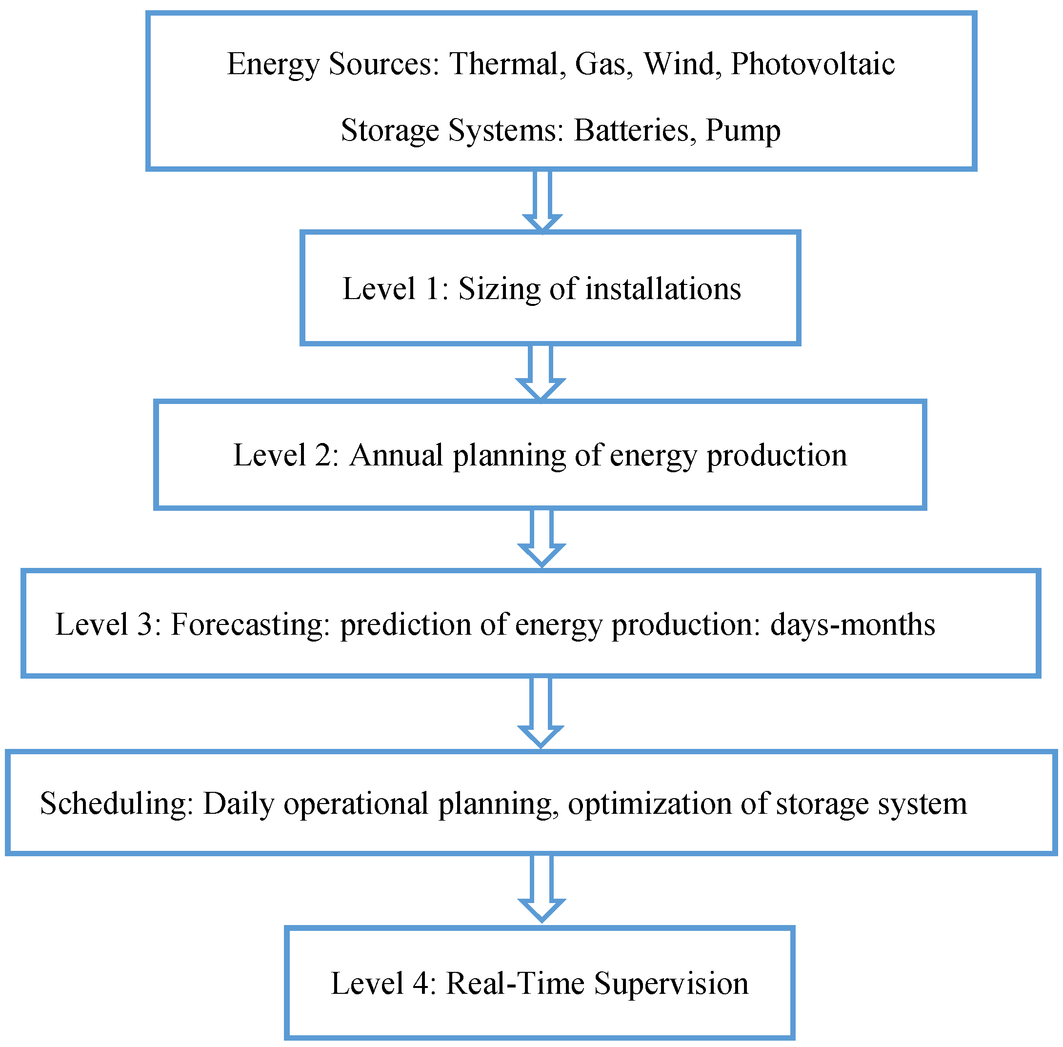
The energy management is performed at the control system level, which is responsible for gathering data to make a good decision. Indeed, the EMS is formed as a hierarchical control architecture, in which the management strategies are organized into several levels considering different time scales [23]. Figure 1 represents the architecture of the EMS.
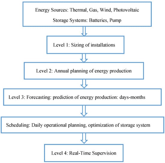
Figure 1.
Hierarchical structure of the EMS in power systems.
The first level consists in the sizing of the installation. The second level of EMS is devoted to annual planning according to the periods of the year. Thus, the annual production schedule depends on the demand and the maintenance forecast. The third level is devoted to planning the production (ranging from 1 day to 1 week). This step consists in the determination of the scheduling power based on the forecasting and the optimization of the used power sources. Finally, the real-time supervision is performed at the last level, in which the power storage is determined in order to guarantee the system services (frequency and voltage). In this paper, the focus will be on the third level, which is devoted to the power forecasting and optimization scheduling of the wind system/PHES. The EMS consists of one forecasting module (day-ahead wind power and load demand predictions) and one optimization module (day-ahead optimization scheduling of the PHES).
3. Power Forecasting
The most essential feature of an optimized EMS in power systems with high shares of RESs is the incorporation of advanced forecasting models. The forecasting model enables uncertainty minimization for both the load power and the renewable power production. Most of the existing works classify the power forecasting depending on the time horizon. Indeed, four time scales have been discussed in the literature. The very short-term forecasts (up to 9 h) are intended to operate in real-time. Short-term forecasts (72 h) [24] are useful in power systems for unit commitment and scheduling and for electricity markets where renewable sources and storage systems can be traded and hedged. Medium-term predictions (from 3 days up to 7 days) [25] are applied to schedule the distributed generator maintenance, the maintenance of the generators, and the unit commitment and to plan the energy storage operations. Moreover, the long-term forecasting deals with periods of months up to years, which is useful for maintenance.
3.1. Kernel Principal Component Analysis (KPCA)
Features selection and extraction is an important task in ML because of the irrelevant data used as part of the training procedure of the prediction system [26,27]. Kernel Principal Component Analysis (KPCA), one of the most used methods for data selection and extraction, was proposed by Schölkopf in [28]. The KPCA is an improved version of the principal component analysis (PCA), which is performed as a linear set of observations [28]. The KPCA performs a nonlinear PCA using an integral operator kernel function, where the key idea of the KPCA is to transform the nonlinear input data into a high dimensional feature space [29].
Given a set of normalized training data , where m is the number of variables, and N is the number of measurements.
PCA is based on the covariance estimation of linear observation xk, k = 1, …, l, xk ϵ ℝ, which is defined as follows [28]:
The KPCA technique performs a nonlinear form of PCA using the integral operator kernel function. It maps the training dataset into a high dimension, where h > >m. The feature space F is defined as [29]:
The mapped data are arranged as:
The covariance matrix C of the nonlinear data of the feature space F is defined as . Equation (3) is used to determine the eigenvalue λ ≥ 0 and the eigenvectors vϵ F\0 satisfying:
The eigenvectors are expressed as:
The kernel matrix () is defined as:
As recommended in [29], the most used kernel function is the radial basis function (RBF), which is given by:
where σ is the width of a Gaussian function. As suggested in [30], a typical choice for σ is the average minimum distance (d) between two points in the training dataset. Using the kernel trick [29], the kernel matrix K is calculated as a function of k(xi, xj) by:
KPCA aims to solve the eigenvector equation in the feature space F. It is assumed that α is the eigenvector of the matrix K, and λ is the eigenvalue.
The matrix of the retained l loading of the KPCA in the feature space F is denoted by and the N-l elements are denoted by .
For a given datum x and its mapped vector , the scores are calculated as:
A measure of the variation within the KPCA model is given by Hotteling’s T2 and the standard squared prediction error (SPE), which are defined as [31,32]:
where A = diag (λ1, λ2, …, λl).
3.2. Random Forest Technique
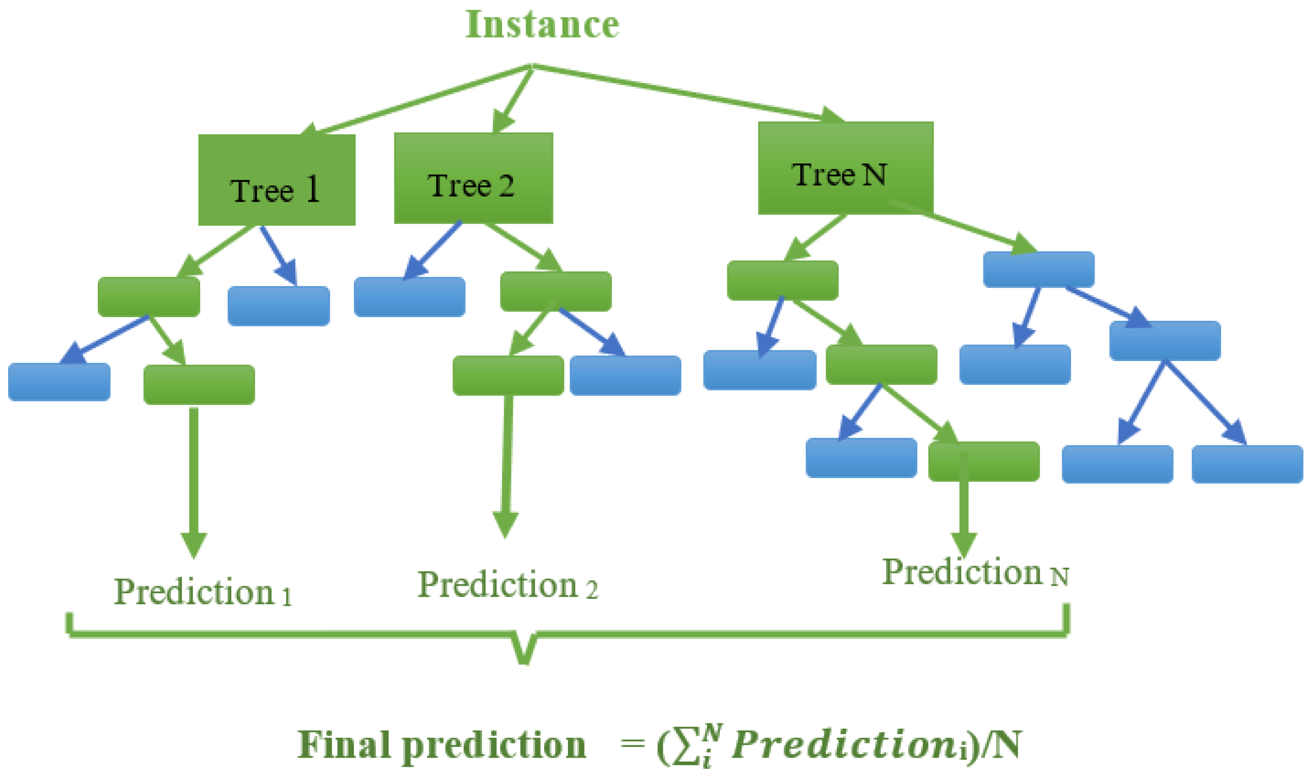
The random forest (RF) is an ensemble technique combining the prediction of several decision trees [33], where the principle is to randomly select a sample of size n with a replacement (bootstrap) from the training set Sn and fit it to a regression tree (bagging) [33]. In this paper, RF is used for the regression problems which aim to predict the wind power generation. The RF technique receives an input vector (X), composed of the training data. Then, the RF algorithm independently builds a number of N regression trees T(X) and thus randomizes the nodes.
Given a sample of training , and in order to construct a regression tree (RT), the input sample data need to be portioned in a set of regions Rj, j = 1, …, N. Moreover, the standard approach to finding a region Rj is CART [34]. CART consists of a binary split along successive variable j according to a selected value s. The splitting of the variable j in terms of the value s is described as:
An optimal choice of j, s must be performed by optimizing the equation below:
The optimal parameters cu and cL are calculated by and .
The response of each tree is to minimize the square error, which is expressed by:
where yi is the measured value and is the predicted value of a tree. which is calculated as the average value by:
After M such trees {R(x)}, the average of the prediction of RF is calculated as:
Figure 2 represents the structure of the RF for regression.

Figure 2.
RF-based prediction structure.
3.3. Evaluation Criteria
Three criteria are proposed to evaluate the accuracy of the wind power forecasting; these are the mean absolute error (MAE), the root mean squared error (RMSE), and the mean absolute percentage error (MAPE), and their mathematical expressions are as below:
where N is the total number of samples, and and are the predicted and the measured values of the wind power, respectively.
These criteria have been considered as the most common assessments of errors in the literature, where the fact that the MAE is the average of the absolute error values makes it the most natural criterion (avoiding error offsets) [34]. Likewise, the RMSE prevents error signs by considering the square root value instead of the absolute value. However, these two evaluation criteria might be irrelevant as they use the raw data instead of the normalized data. Thus, the MAPE might overcome this drawback by averaging the sum of the errors divided by the actual power value [34]. Nevertheless, the MAPE might tend to infinity when the actual power value is around zero (intermittent power sources).
4. Short-Term Wind Energy Forecasting Using Random Forest
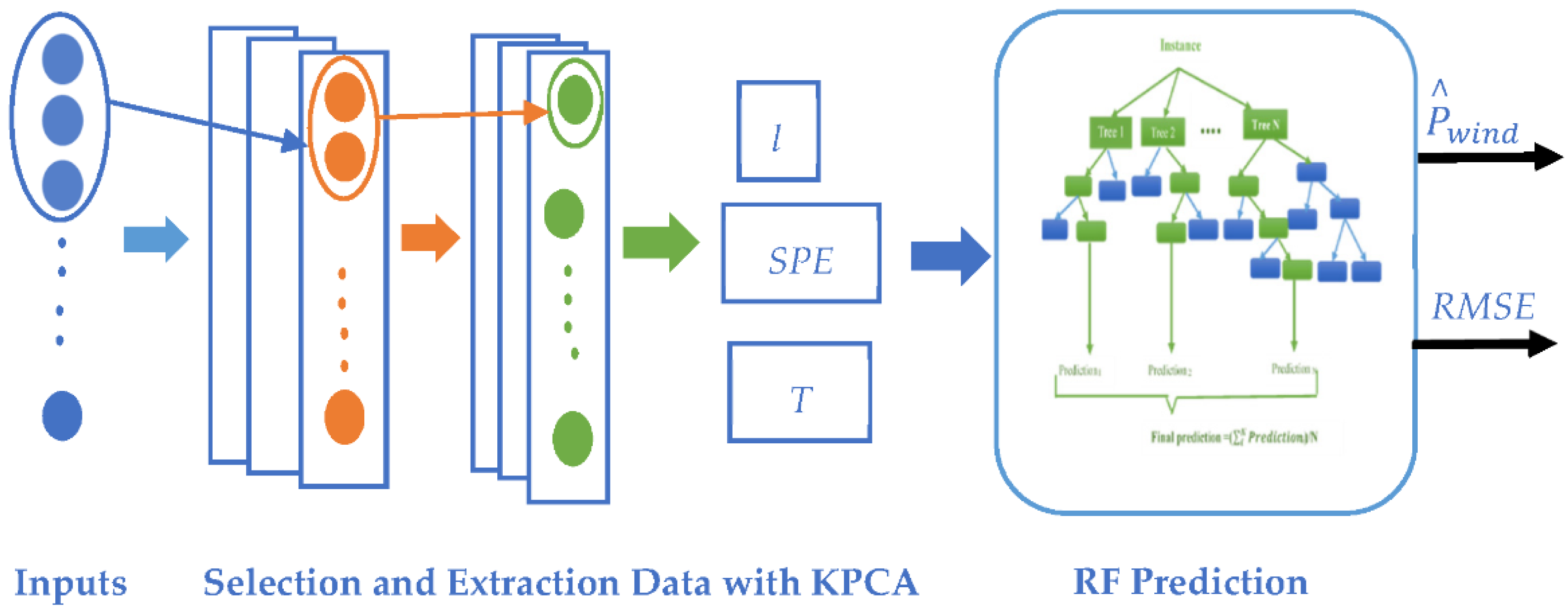
The methodology of wind energy prediction using RF is illustrated in Figure 3. First, the meteorological conditions data (wind speed, temperature, and pressure) are considered as inputs. Then, the selection and extraction of the useful information from the input data are performed using the KPCA technique. Afterwards, the RF technique is implemented to forecast the wind power generation.

Figure 3.
Flowchart of the proposed wind energy forecasting.
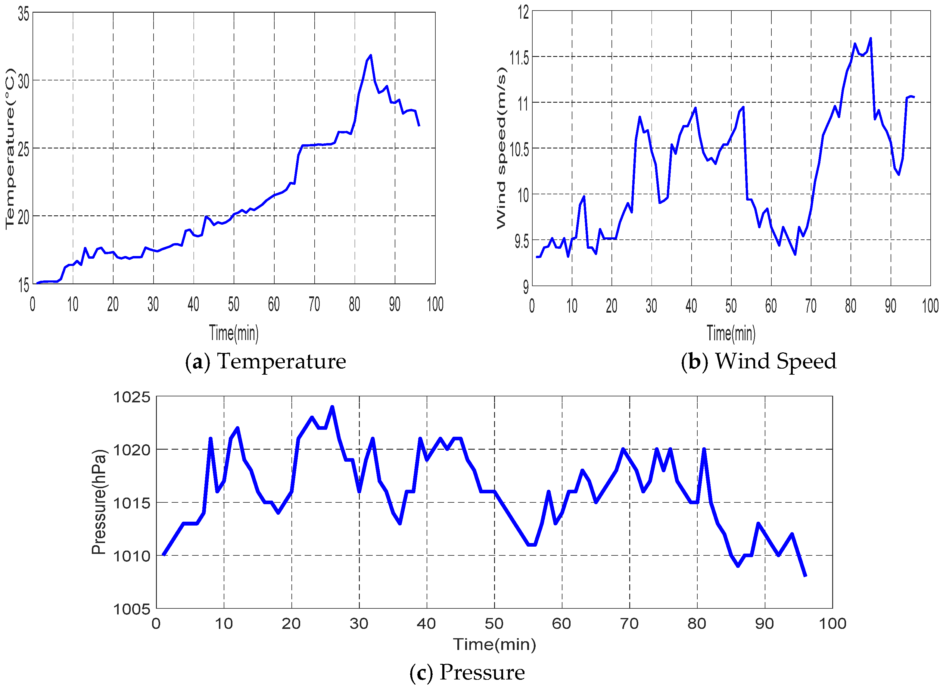
Based on the KPCA results, the RF training was used to train the candidate algorithm and to fit the model, and the test set was used to generate the wind power values. Two factors were taken into consideration for the RF training; these are the number of trees and the number of leaves. Finally, several well-known metrics were used to assess the performance of the proposed algorithm, where repetitive training subsets were generated by extraction and substitution (the size of the training subsets is equal to the size of the initial training dataset). Figure 4 shows one-day (samples were taken every 15 min for 24 h) variations of the meteorological data (temperature, wind speed, and pressure), while the short-term wind power forecasting (a day ahead) is illustrated in Figure 5.
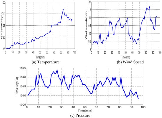
Figure 4.
Input data.

Figure 5.
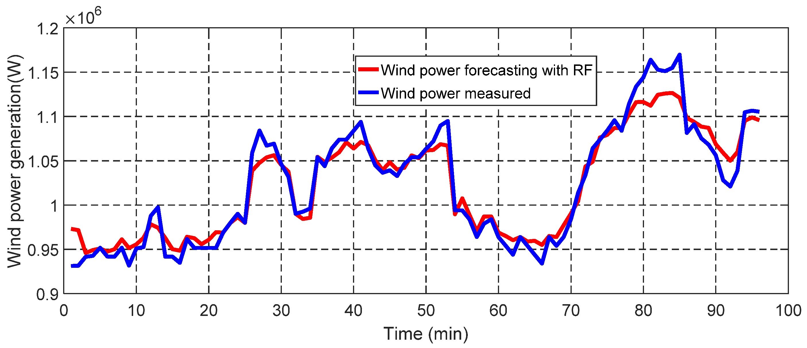
Forecasted wind power generation using RF.
The day-ahead RF forecast results presented in Figure 5 show the predicted wind power (samples were taken every 15 min), while taking all the three possible inputs (wind speed, temperature, and pressure). The forecast is accurate in most situations, except during sharp and sudden variations of the measured signal. As can be seen from this figure, the RF could be considered successful in forecasting both low and high wind power values. Moreover, one can notice that the RF algorithm could adapt to the change in standard deviation and successfully forecast power based on the meteorological conditions.
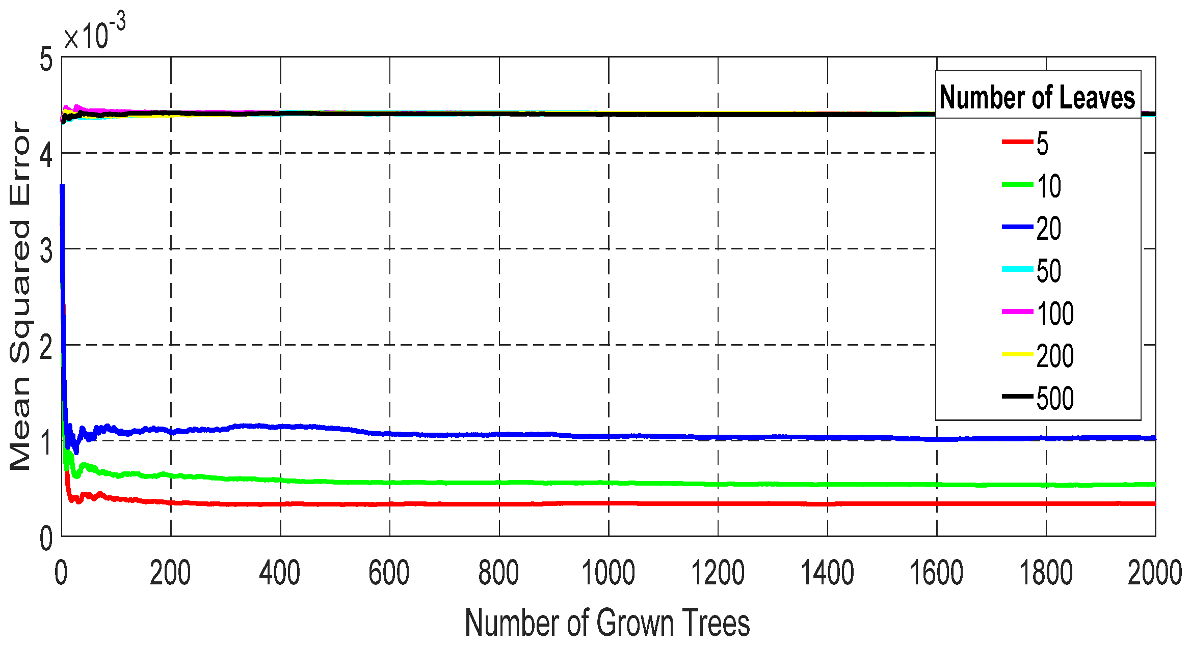
In addition, the behavior of the RF process depends on two main parameters, which are the number of trees in the forest and the maximum of the tree depth (the number of leaves). In this research, the numbers of trees and leaves were increased until the error stabilized. The RMSE of the RF response, with regard to the training data for the day-ahead prediction, was taken into consideration. The result of the RMSE for the wind energy prediction is given in Figure 6.
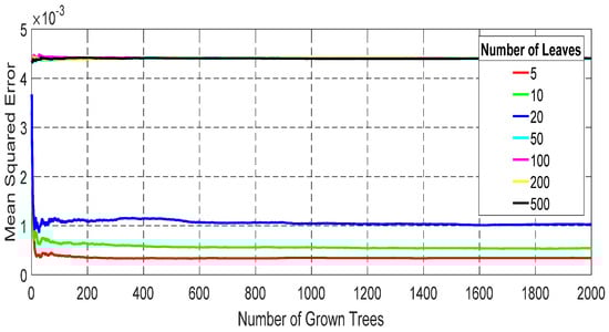
Figure 6.
RMSE representation.
One can notice that the RMSE is decreased when more trees are added, while it remains constant after reaching 200 trees. Moreover, the accuracy is increased when a low number of leaves is used (i.e., the RMSE is minimal when 5 leaves are used instead of 10). In addition, the evaluation of the RF performance for wind power prediction based on the RMSE, MAE, and MAPE values is illustrated in Table 1.

Table 1.
RF Results Evaluation.
It is worth noting that both the RMSE and the MAE were increased when the number of leaves rose. Moreover, one can notice that the performance results of the RF are highly dependent on the number of trees and leaves. Then, the RMSE and MAE decreased rapidly when adding more trees. In contrast, the RF gives a good performance as the number of leaves decreases. Then, the RMSE, MAE, and MAPE are 2%, 6%, and 3%, with the number of trees and leaves equal to 200.
5. Modelling of the Grid-Connected Wind Farm-PHES
For the grid-connected system, the priority is given to the injection of the generated wind power to the grid. The PHES is functioning in two modes of operation to compensate for the imbalance between the wind power production and the load power demand. In the pumping mode, the centrifugal pumps operate during the wind power overproduction. As a result, the pump moves the water from the lower reservoir to the upper one. In the generating mode, the hydraulic generator produces electricity during the discharge of the reservoir (Figure 7).
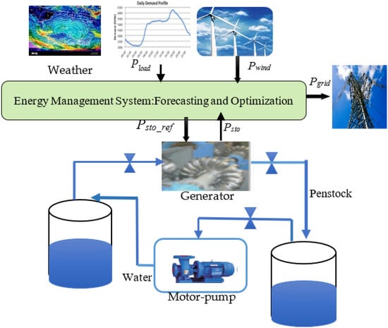
Figure 7.
Configuration of the studied wind farm coupled with the PHES.
5.1. Wind Farm Modelling
The mathematical relationship between the wind power generation and the cube of the wind speed is expressed as follows [35].
where ρ is the air density, Pwind is the power extracted from the wind turbine, v is the wind speed in m/s, S is the area swept by the rotor of the wind turbine in m2, and Cp is the coefficient of the wind turbine.
5.2. PHES Modelling
The operation of the used PHES was described in [36]. The variation of the flow rate of the reservoir is formulated as:
The expression of the head of the reservoir is written as follows:
The storage energy of the reservoir is formulated as:
The reservoir volume is obtained by:
6. Optimization of the EMS for the Wind Farm Coupled with PHES
As previously mentioned, the EMS is designed to determine the operational planning a day ahead, when the fixed generators and storage sources will be operational. Moreover, the EMS determines the power generated by each generation source for the next day. Consequently, the EMS guarantees the robustness against the uncertainties of renewable energy and the balance of energy in the power system. In this paper, an EMS of a wind farm coupled with PHES is developed to provide the sufficient amount of reserve (storage PHES) to satisfy all the operational constraints and then guarantee the supply–demand balance for the next day.
6.1. Day-Ahead Optimization
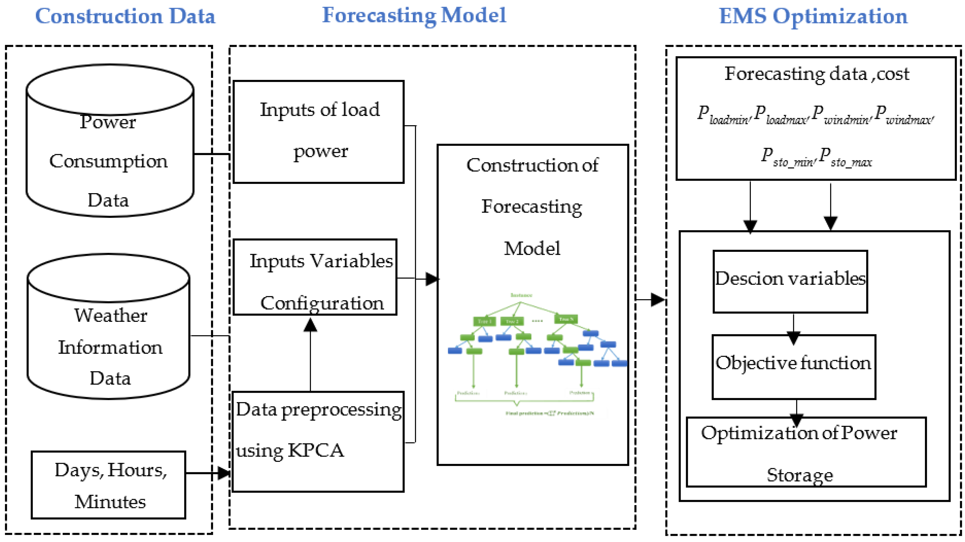
The energy management optimization enhances the daily operational planning with respect to a cost function to be optimized. In this research, the strategy of EMS optimization consists in developing a dynamic optimization technique that considers the forecasted wind power and load demand power as two input variables, as well as the storage power and the reservoir volume as two decision variables; then, an objective function based on the profit cost maximization is applied. Figure 8 represents the architecture of the proposed management optimization.
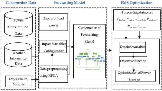
Figure 8.
Architecture of the proposed EMS.
6.1.1. Problem Formulation
The use of optimization techniques first requires the defining of the problem which represents the variables decision, the constraints, and the objective function.
6.1.2. Variables Decision
The variables decision comprises the variables defined by the optimization technique to reach the optimal solution. They are represented by:
- Psto: The storage power generated is considered as the variable that describes the way of storing and discharging the reservoir. Moreover, it allows the satisfying of the load power. This power represents both the storage power in turbining mode, Phyd, and the storage power in the pumping mode, Ppump.
- Vol: The volume of the reservoir from which the storage capacity is defined.
6.1.3. Constraints
The constraints of the joint operation of the wind farm/PHES are formulated in Table 2.
Table 2.
System Constraints.
6.1.4. Objective Function
The objective of the optimization problem is to find the storage power of the PHES set point to satisfy the power demand by maximizing the profit cost.
The storage reference power is defined by:
where Pgrid is the power fed to the grid, and Pwind is the generated wind power.
The power generated by the wind farm/PHES system is expressed as follows:
The objective function which aims to maximize the cost of the profit is formulated as follows:
where ηpump is the efficiency of the pumped station, ηhyd is the efficiency of the hydraulic turbine, Δt is the time period, ρ (kg/m3) is the density, g (N/kg) is the acceleration, vol (m3) is the volume of the reservoir, ΔQ (m3/s) is the variation of flow rate, and S (m2) is the surface of the reservoir.
6.2. Nonlinear Programming-Based EMS Optimization
Nonlinear programming is a method for solving the nonlinear optimization problems with continuous variables. The general form of the optimization problem in its deterministic version is written as follows:
- Min f(x); x∈ RN
- The constraints are g(x) ≤ 0 and Lb < x< Ub
where x represents the vector of the decision variables, f(x) is the objective function, and g(x) is the set of constraints to which the variables are subjected; it is a question of defining the domain of constraints called the feasibility domain; Lb is the lower bound and Ub is the upper bound of the decision variable.
The optimization by NLP allows the finding of a global optimum in the case where the objective function of the problem is a convex function, otherwise it provides a local optimum. The particularity of this method is that it strongly depends on the initial conditions which consist in choosing an initial solution in order to accelerate the convergence towards the optimal point [37]. However, this method has the disadvantage of stopping at the first local minimum found. The approach developed in this paper is based on the NLP technique to optimize the EMS of the wind farm coupled with PHES storage. This optimization is conducted via the objective function of Equation (31), under the constraints obtained in Table 2. The non-linearity in our case appeared during the optimization process. Indeed, it is not possible to know a priori what the sign of the optimal storage power will be, and the coefficients of the Vol variable would depend on the sign of the Psto solution, which represents a nonlinear constraint.
6.3. Results and Discussion
The Elhierro station (located in Spain) was considered as a case study in this work. This station consists of a wind farm coupled with a PHES. The wind farm is composed of a set of five aero generators (Enercon E-70) with a rated power of 2.3 MW each (total power of 11.5 MW). The pumped station contains two 1500 kW and six 500 kW pumps (total power of 6 MW). Four Pelton groups of 2.38 MW each make the hydraulic turbine capacity equal to 11.32 MW, where the water capacity of the reservoir is 380,000 m3, and the head of the dam height is equal to 680 m [38].
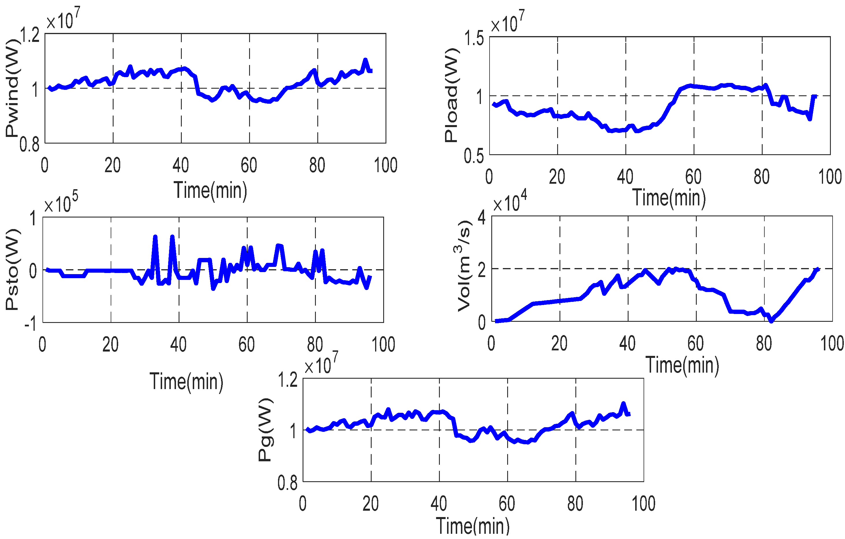
The nonlinear optimization problem is solved using the MATLAB toolbox “Optimization”. A predefined function “fmincon” is used to solve the optimization problem [39]. Moreover, the results were obtained every 15 min in order to find a daily operating and a long-term (7 days) optimization strategy for both the wind farm and the PHES. The simulation results of the NLP optimization are shown in Figure 9 (1-day results) and Figure 10 (7-day results).

Figure 9.
One-day optimization results using the proposed NLP.
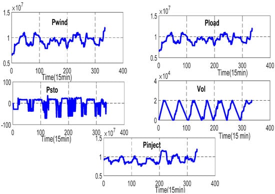
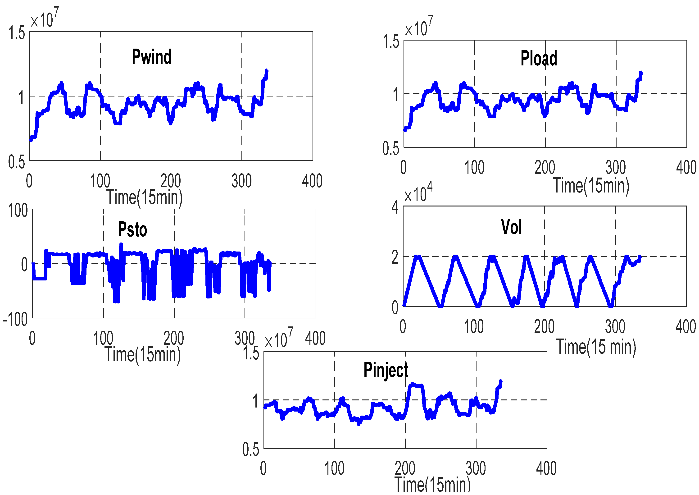
Figure 10.
Seven-day optimization results using the proposed NLP.
From Figure 9, one can notice that the imbalance between the forecasted wind power production and the load power is predominantly positive (over-production of wind energy). The excess of power has been stored in the high reservoir. On other hand, during the under-production period, one can notice the reduction in the pumping operation between samples 40 and 50. In addition, the change in the PHES operation can be observed (Psto) when the plant operates as a generator between samples 50 and 80. In this case, the under-production is compensated after sample 80 until the end. The same interpretation is valid for longer time-horizon optimization (Figure 10), which shows that the reservoir is charged during the under-production and discharged during the over-production of wind energy. The evaluation of the optimization from NLP is given in Table 3 and Table 4, where the penalty and profit costs are displayed for one day according to the starting point and the optimization period. The two starting points are thus generated by considering a vector of 96 samples according to the lower bound Lb and the upper bound Ub.
Table 3.
One-Day NLP Evaluation.
Table 4.
Seven-day NLP Evaluation.
Two different starting points taken arbitrarily at the level of Ib and Ub are considered to launch the NLP algorithm. The NLP is characterized by a very reduced computation time, but the non-convergence imposes the necessity to carry out a great number of launches to obtain a satisfactory optimum. One can notice that in both cases the solution of the problem by NLP is assured, and the maximization of income is reached. One can notice that the constraints imposed on the optimization problem are respected. Moreover, it has been shown that the NLP optimization gives good performances in terms of cost and computation time.
7. Conclusions
This paper presented an optimized energy management strategy (EMS) for a grid-connected wind energy production farm, including a pumped hydro storage system (PHES). The EMS design is divided into two modules: one random forest (RF)-based forecasting module for day-ahead wind power and load demand predictions and one optimization module for the day-ahead PHES scheduling. In order to select and extract the most relevant meteorological factors (wind, temperature, and atmospheric pressure) to be included in the predictor, a kernel principal component analysis (KPCA) technique was used. The KPCA method is based on the transformation of data to high-dimensional features space.
After preprocessing and selecting the input data, the RF technique was applied to predict the wind energy production in a day-ahead horizon (regression is based on construction of a number of trees and randomizing the nodes). The presented results showed that the RF technique is well capable of predicting wind power with low errors. Based on the obtained predictions, the management optimization was performed in a day-ahead horizon. Then, after formatting the optimal management problem, an explicit nonlinear programming (NLP) method was applied to obtain an optimal storage power reference set. The results obtained on the EMS optimization show that the NLP method gives a good performance in terms of profit cost and computation time.
Author Contributions
Conceptualization, J.J., M.T. and M.M.; methodology J.J., M.T. and M.M.; software, J.J.; validation, J.J., M.T. and M.M.; formal analysis, J.J., M.T. and M.M.; investigation, J.J.; resources, J.J.; data curation, J.J.; writing—original draft preparation, J.J.; writing—review and editing, J.J., M.T. and M.M.; visualization, M.F.M. and W.S.; supervision, M.T., M.M., M.F.M. and W.S.; project administration, M.M.; funding acquisition, M.M. All authors have read and agreed to the published version of the manuscript.
Funding
This work was supported by the Qatar National Research Fund (a member of the Qatar Foundation).
Conflicts of Interest
The authors declare no conflict of interest.
Nomenclature
| Renewable Energy Source | RES | Deep Neural Network | DNN |
| Energy Management System | EMS | Regression Tree | RT |
| Energy Storage System | ESS | Classification and Regression Tree | CART |
| Pumped Hydro Energy System | PHES | Squared Prediction Error | SPE |
| Random Forest | RF | Mean Absolute Error | MAE |
| Kernel Principal Component Analysis | KPCA | Root Mean Squared Error | RMSE |
| Non-Linear Programming | NLP | Mean Absolute Percentage Error | MAPE |
| Compressed Air Energy Storage | CAES | Input data | x |
| Machine Learning | ML | Output data | y |
| Support Vector Regression | SVR | Measured Wind Power | Pwind |
| Multiple Linear Regression | MLR | Predicted Wind power | |
| Decision Tree | DT | Rate | Q |
| Feature Extraction and Selection | FES | Volume of reservoir | Vol |
| Photovoltaic | PV | Reservoir Energy | E |
| Independent Component Analysis | ICA | Head of Reservoir | H |
| Partial Least Squares | PLS | Pumped Power | Ppump |
| Deep Learning | DL | Hydraulic Power | Phyd |
| Recurrent Neural Network | RNN | Storage Power | Psto |
| Deep Belief Network | DBN | Grid Power | Pgrid |
References
- Reihani, E.; Sepasi, S.; Roose, L.R.; Matsuura, M. Energy management at the distribution grid using a Battery Energy Storage System(BESS). Int. J. Electr. Power Energy Syst. 2016, 77, 337–344. [Google Scholar] [CrossRef]
- Weitemeyer, S.; Kleinhans, D.; Vogt, T.; Agert, C. Integration of Renewable Energy Sources in future power systems: The role of storage. Renew. Energy 2015, 75, 14–20. [Google Scholar] [CrossRef]
- Anagnostopoulos, J.S.; Papantonis, D.E. Pumping station design for a pumped-storage wind-hydro power plant. Energy Convers. Manag. 2007, 48, 3009–3017. [Google Scholar] [CrossRef]
- Najeebullah; Zameer, A.; Khan, A.; Javed, S.G. Machine Learning based short term wind power prediction using a hybrid learning model. Comput. Electr. Eng. 2015, 45, 122–133. [Google Scholar] [CrossRef]
- Sasser, C.; Yu, M.; Delgado, R. Improvement of wind power prediction from meteorological characterization with machine learning models. Renew. Energy 2021, 183, 491–501. [Google Scholar] [CrossRef]
- Heinermann, J.; Kramer, O. Machine Learning Ensembles for Wind Power Prediction. Renew. Energy 2015, 89, 671–679. [Google Scholar] [CrossRef]
- Masini, R.P.; Medeiros, M.C.; Mendes, E.F. Machine Learning Advances for Time Series Forecasting; 802v3.econ.EM.9; Wiley: Hoboken, NJ, USA, 2021. [Google Scholar]
- Dhibi, K.; Fezai, R.; Mansouri, M.; Trabelsi, M.; Bouzrara, K.; Nounou, H.; Nounou, M. A Hybrid Fault Detection and Diagnosis of Grid-Tied PV Systems: Enhanced Random Forest Classifier Using Data Reduction and Interval-Valued Representation. IEEE Access 2021, 9, 64267–64277. [Google Scholar] [CrossRef]
- Dhibi, K.; Fezai, R.; Mansouri, M.; Trabelsi, M.; Kouadri, A.; Bouzara, K.; Nounou, H.; Nounou, M. Reduced Kernel Random Forest Technique for Fault Detection and Classification in Grid-Tied PV Systems. IEEE J. Photovolt. 2022, 10, 1864–1871. [Google Scholar] [CrossRef]
- Sheriff, M.Z.; Botre, C.; Mansouri, M.; Nounou, H.; Nounou, M.; Karim, M.N. Process monitoring using data-based fault detection techniques: Comparative studies. In Fault Diagnosis and Detection; InTech: Rijeka, Croatia, 2017; pp. 237–261. [Google Scholar]
- Li, S.Z.; Lu, X.; Hou, X.; Peng, X.; Cheng, Q. Learning multiview face subspaces and facial pose estimation using independent component analysis. IEEE Trans. Image Process. 2005, 14, 705–712. [Google Scholar] [CrossRef]
- Kembhavi, A.; Harwood, D.; Davis, L.S. Vehicle detection using partial least squares. IEEE Trans. Pattern Anal. Mach. Intell. 2011, 33, 1250–1265. [Google Scholar] [CrossRef]
- Cao, L.; Chua, K.; Chong, W.; Lee, H.; Gu, Q. A Comparison of PCA, KPCA and ICA for Dimensionality Reduction in Support Vector Machine; Elsevier B.V.: Amsterdam, The Netherlands, 2003. [Google Scholar] [CrossRef]
- Salcedo-Sanz, S.; Cornejo-Bueno, L.; Prieto, L.; Paredes, D.; García-Herrera, R. Feature selection in machine learning prediction systems for renewable energy applications. Renew. Sustain. Energy Rev. 2018, 90, 728–741. [Google Scholar] [CrossRef]
- Deng, X.; Shao, H.; Hu, C.; Jiang, D.; Jiang, Y. Wind Power Forecasting Methods Based on Deep Learning: A Survey. Comput. Model. Eng. Sci. CMES 2020, 122, 273–301. [Google Scholar] [CrossRef]
- Parastegari, M.; Hooshmand, R.A.; Khodabakhshian, A.; Forghani, Z. Joint operation of wind farms and pump-storage units in the electricity markets: Modeling, simulation and evaluation. Simul. Model. Pract. Theory 2013, 37, 56–69. [Google Scholar] [CrossRef]
- Gao, J.; Zheng, Y.; Li, J.; Zhu, X.; Kan, K. Optimal model for complementary operation of a photovoltaic-wind pumped storage system. Hindawi Math. Probl. Eng. 2018, 2018, 5346253. [Google Scholar] [CrossRef]
- Hozouri, M.A.; Abbaspour, A.; Fotuhi-Firuzabad, M.; Moeini-Aghtaie, M. On the use of pumped storage for wind energy maximization in transmission-constrained power systems. IEEE Trans. Power Syst. 2015, 30, 1017–1025. [Google Scholar] [CrossRef]
- Shi, N.; Zhou, S.; Su, X.; Yang, R.; Zhu, X. Unit Commitment and Multi-Objective Optimal Dispatch Model for Wind-Hydro-Thermal Power System with Pumped Storage. In Proceedings of the 2016 IEEE 8th International Power Electronics and Motion Control Conference (IPEMCECCE Asia), Hefei, China, 22–26 May 2016. [Google Scholar]
- An, L.N.; Quoc-Tuan, T. Optimal energy management for an island micro grid by using Dynamic programming method. In Proceedings of the 2015 IEEE Eindhoven Power Tech, Eindhoven, The Netherlands, 29 June–2 July 2015. [Google Scholar]
- Duque, J.; Castronuovo, E.D.; Sanchez, I.; Usaola, J. Optimal operation of a pumped-storage hydro plant that compensates the imbalances of a wind power producer. Electr. Power Syst. Res. 2011, 81, 1767–1777. [Google Scholar] [CrossRef]
- Kumar, M.; Saini, P.; Kumar, N. Optimization of wind-pumped storage hydropower system. Int. J. Eng. Technol. Manag. Appl. Sci. 2016, 4, 67–75. [Google Scholar]
- Robyns, B.; Davigny, A.; Saudemont, C. Methodologies for supervision of hybrid energy sources based on storage system—A survey. Math. Comput. Simul. 2013, 91, 52–71. [Google Scholar] [CrossRef]
- Foley, A.M.; Leahy, P.G.; Marvuglia, A.; McKeogh, E.J. Current methods and advances in forecasting of wind power generation. Renew. Energy 2011, 37, 1–8. [Google Scholar] [CrossRef]
- Costa, A.; Crespo, A.; Navarro, J.; Lizcano, G.; Madsen, H.; Feitosa, E. A review on the young history of the wind power short-term prediction. Renew. Sustain. Energy Rev. 2008, 12, 1725–1744. [Google Scholar] [CrossRef] [Green Version]
- Blum, A.L.; Langley, P. Selection of relevant features and examples in Machine Learning. Artif. Intell. 1997, 97, 245–271. [Google Scholar] [CrossRef]
- Weston, J.; Mukherjee, S.; Chapelle, O.; Pontil, M.; Poggio, T.; Vapnik, V. Feature selection for SVMs. In Proceedings of the 13th International Conference on Neural Information Processing Systems; MIT Press: Cambridge, MA, USA, 2000. [Google Scholar]
- Schölkopf, B.; Smola, A.; Müller, K.R. Nonlinear component analysis as a kernel eigenvalue problem. Neural Comput. 1998, 10, 1299–1319. [Google Scholar] [CrossRef]
- Harkat, M.F.; Mansouri, M.; Nounou, M.; Nounou, H. Fault detection of uncertain nonlinear process using interval-valued data-driven approach. Chem. Eng. Sci. 2019, 205, 36–45. [Google Scholar] [CrossRef]
- Rathi, Y.; Dambreville, S.; Tannenbaum, A. Statistical shape analysis using kernel pca. In Image Processing: Algorithms and Systems, Neural Networks, and Machine Learning; International Society for Optics and Photonics: Washington, DC, USA, 2006; Volume 6064, p. 60641B. [Google Scholar]
- Choi, S.W.; Lee, C.; Lee, J.-M.; Park, J.H.; Lee, I.-B. Fault detection and identification of nonlinear processes based on kernel pca. Chemom. Intell. Lab. Syst. 2005, 75, 55–67. [Google Scholar] [CrossRef]
- Cui, P.; Li, J.; Wang, G. Improved kernel principal component analysis for fault detection. Expert Syst. Appl. 2008, 34, 1210–1219. [Google Scholar] [CrossRef]
- Alonso, Á.; Torres, A.; Dorronsoro, J.R. Random Forests and Gradient Boosting for Wind Energy Prediction; Springer International Publishing: Cham, Switzerland, 2015. [Google Scholar] [CrossRef]
- Lahouar, A.; Slama, J.B.H. Hour-ahead wind power forecast 1 based on random forests. Renew. Energy 2017, 109, 529–541. [Google Scholar] [CrossRef]
- Baumgart, A. Mathematical model of wind turbine. J. Sound Vib. 2002, 251, 1–12. [Google Scholar] [CrossRef]
- Jamii, J.; Abbes, D.; Mimouni, M.F. Joint operation between wind power generation and pumped hydro energy storage in the electricity market. Wind. Eng. 2019, 45, 50–62. [Google Scholar] [CrossRef]
- Bridier, L.; David, M.; Lauret, P. Optimal design of a storage system coupled with intermittent renewable. Renew. Energy 2014, 67, 2–9. [Google Scholar] [CrossRef]
- Quintero, F.C.; Padron, J.M.; Dominguez, E.M.; Santana, M. Renewable Hydro-Wind Power system for small Islands: The Elhierro Case. Int. J. Tech. Phys. Probl. Eng. ISS 2016, 8, 1–7. [Google Scholar]
- Whitefoot, J.W.; Mechtenberg, A.R.; Peters, D.L.; Papalambros, P.Y. Optimal Component Sizing and Forward-Looking Dispatch of an Electrical Microgrid for Energy Storage Planning. In Proceedings of the ASME 2011 International Design Engineering Technical Conferences and Computers and Information in Engineering Conference, Washington, DC, USA, 28–31 August 2011. [Google Scholar]

Publisher’s Note: MDPI stays neutral with regard to jurisdictional claims in published maps and institutional affiliations. |
© 2022 by the authors. Licensee MDPI, Basel, Switzerland. This article is an open access article distributed under the terms and conditions of the Creative Commons Attribution (CC BY) license (https://creativecommons.org/licenses/by/4.0/).