Travel Time Prediction for Traveler Information System in Heterogeneous Disordered Traffic Conditions Using GPS Trajectories

Abstract

Precise travel time prediction allows travelers and system controllers to be aware of the future conditions on roadways and helps in pre-trip planning and traffic control strategy formulation to lessen the travel time and mitigate traffic congestion problems. This research investigates the possibility of using the GPS trajectory dataset for travel time prediction in Indian traffic conditions having heterogeneous disordered traffic and improvement in prediction accuracy by shifting from the traditional historical average method to modern machine learning algorithms such as linear regressions, decision tree, random forest, and gradient boosting regression. The present study uses massive location data consisting of historical trajectories that were collected by installing GPS devices on the probe vehicles. A 3.6 km long stretch of the Delhi–Noida Direct (DND) flyway is selected as a case study to predict the travel time and compare the performance as well as the efficiency of various travel time prediction algorithms.

1. Introduction

Modern traveler information systems and location-based navigation systems are dependent on the ability to precisely predict route travel time in the present and near future. The travel time of the route may vary significantly from hour to hour, day in and day out, because of the variations in traffic demand, variations in capacity due to incidents, roadwork, or adverse weather, vehicle–vehicle variability due to differences in driver behavior such as aggressiveness and lane choices [1], and the presence of traffic congestion in urban areas [2]. As a result, it is essential to depend on extensive traffic data to precisely predict travel times. With accurate travel time predictions, travelers can make more informed decisions about trip generation and routing, resulting in more consistent traffic conditions and alleviating traffic congestion problems [3]. These more informative decisions can also help to reduce greenhouse gas emissions as researchers have found that congested conditions can have up to 40% higher CO₂ emissions than steady-state conditions [4].

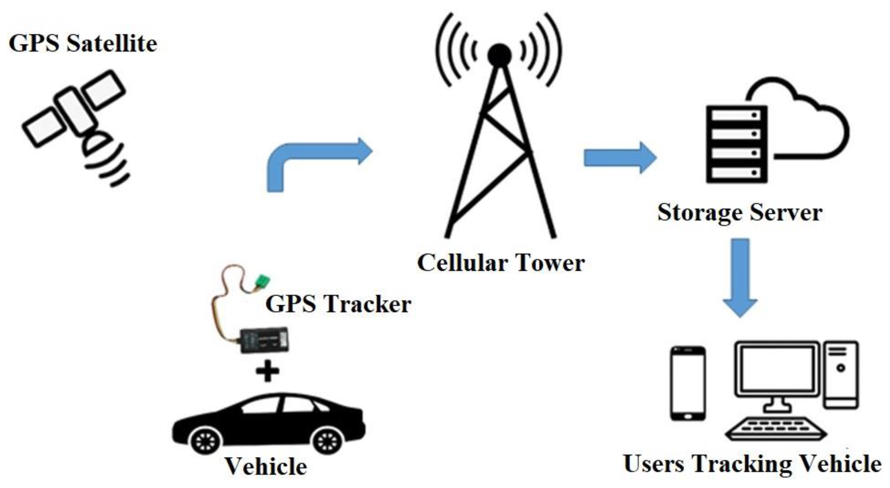
Traditional methods of monitoring traffic conditions using stationary sensors such as the induction loop, traffic cameras, and license plate detectors require the installation of sensors/devices on the city’s selected roads and highways. These data collection methods are usually limited, especially in developing countries, because of the significant investment and challenges that are involved in controlling and coordinating the sensors. Due to the growth in popularity of GPS devices over the last decade, large-scale traffic data that were collected by GPS-enabled vehicles can now be used to estimate and predict traffic conditions. In the present study, the authors investigate the possibility of using the data that were collected by GPS-enabled vehicles for travel time prediction in Indian traffic conditions. Below we provide a review of travel time prediction studies.

Early research on travel time prediction used mathematical statistics [5,6,7]. For instance, a linear model with varying coefficients was proposed by Zhang and Rice [8]. Statistical models are commonly employed for travel time prediction because of the ease of implementation and low computational effort requirement. However, the accuracy of these models is usually low [3].

Another traditional travel time prediction technique, namely, historical average models, assumes that present traffic conditions will remain constant and forecast current and future travel times that are based on previous trip travel time data. Therefore, these models are useful only in locations where traffic is relatively steady over time or where congestion is limited, such as in rural areas [9]. In the scientific literature, these models are used as a baseline only because of its poor prediction ability and unrealistic assumption that travel time will remain constant indefinitely.

Recent studies on travel time estimation and prediction are based on data-driven models because of their ability to determine the function relating explicative variables with target variables from the data itself, the ability to extract hidden input features/patterns, and the advancement of technology for harnessing and processing traffic data. These include machine learning methods such as linear regression, decision tree (DT), random forest (RF), and gradient boosting regressor (GBR). Machine learning algorithms can capture the complex and underlying relationships between various factors even when their relationships are not readily apparent [10]. Table 1 summarizes the travel time prediction studies which used modern machine learning methods, whereas Table 2 summarizes the travel time prediction studies that have been done in India. Importantly, both tables state the limitations of these studies.

Studies [11,12,13] that were done in countries such as China and the USA show that using modern machine learning algorithms improves the accuracy of travel time forecasts. Notably, we found a few major limitations of previous studies. The first limitation is that a majority of studies focused on homogeneous traffic streams and heterogeneous disordered traffic streams (as prevalent in developing countries such as India, Pakistan, Nepal, Bhutan, Bangladesh, Sri Lanka etc.) were under explored. By heterogeneity, the authors mean that the traffic stream consists of various types of vehicles such as cars, motorized two wheelers, buses, trucks, motorized three wheelers, and non-motorized vehicles having notably different physical and dynamic characteristics that leads to differences in their driving behavior. For example, driver behavior of buses will differ from motorcycles because buses have a larger size and lower maneuverability as compared to motorcycles. Moreover, disordered traffic can be characterized by a lower extent of vehicle following, staggered following (one vehicle behind two leaders but placed in between them), a larger extent of lateral movements, and situations such as vehicles suddenly cutting in front of other vehicles and excessive overtaking. It is highly likely that this heterogeneity and disorderliness may introduce the random variability in travel time, which complicates and toughens the travel time prediction process as compared to homogeneous traffic streams. Hence, there is a need to examine existing travel time prediction models, to unearth their applicability in heterogeneous and disordered traffic streams. The second limitation is that most studies focused on the public transport vehicles only. The travel time of public transport vehicles and other vehicles will be different due to buses’ requirement to schedule adherence, dwell time, acceleration/deceleration time, bus queuing time, etc. [14]. In addition, as mentioned before, the driver behavior of these vehicles will be different in the heterogeneous disordered traffic conditions. Importantly, consideration of travel time values of almost all types of vehicles that are present in the traffic stream will assist in predicting realistic travel time values thereby presenting a comprehensive picture to researchers and policy-makers. In addition, we also noticed that a large dataset (say around 1 year data) was not utilized in most of the studies. Large datasets can facilitate in predicting realistic travel times since they capture more variability in the data. Also, in the literature, most of the studies predict travel time for the short-term only. Long-term travel time prediction plays a critical role in transportation planning as such it can improve transport decisions [15], facilitate the appraisal of transportation projects [16], benefit traffic navigation [17], reduce travel costs [18], aid vehicle dispatching [19], and so on.

Motivated by the limitations of previous studies, this study compares the performance as well as efficiency of machine learning-based travel time prediction algorithms using a large GPS dataset of heterogeneous disordered traffic streams. Moreover, this study uses the travel time data of all types of vehicles that are present in the traffic stream for travel time prediction. Furthermore, this study predicts the travel time for the long-term. The analysis and results that are presented in this paper are based on the consideration of heterogeneous traffic data, comparison of machine learning algorithms, inclusion of data of all vehicles that are present in the traffic stream, the use of large dataset, and long-term predictions and has the potential to attract wide audience, not limited to the Indian subcontinent.

The rest of the paper is organized as follows: Section 2 provides the details of the data collection process and pre-processing that was done to obtain the travel time dataset that was used in the present study. Section 3 shows the data analysis that was performed on the dataset to obtain pattern/trend of daily and hourly variation of the travel time. This section also provides insights to the travel time variation in heterogeneous disordered traffic conditions that are prevalent in developing countries. Section 4 describes the methodology that was used for the development of travel time prediction models using traditional historical average method and modern machine learning algorithms. Section 5 shows the results of the comparison of performance of algorithms that were used in the present study by using mean absolute percentage error (MAPE) and satisfaction rate (SR). This section also compares the efficiency of the machine learning algorithms that were used in the current study. Finally, Section 6 concludes the findings of the present study. This section also presents the limitation and recommendations of the present study.

Table 1. Summary of travel time prediction studies using modern machine learning methods.

Study	Data Source	Location	Data Type	Roadway Category	Prediction Method	Types of Vehicles Considered	Dataset Duration/Size	Limitations
[20]	GPS	N/A	TS	N/A	RF	Car	500 Hours	Used one vehicle category and simulated data, no comparison of algorithms
[21]	GPS	Bangkok, Thailand	TT, GPS	Highway	BP NN	N/A	One month	No comparison of algorithms
[22]	GPS Data	Delft, Netherlands	Vehicle position, TS	Urban Road	State-Space NN	Car	7 Round trips	Used one vehicle category and simulated data, no comparison of algorithms
[23]	INRIX Company	Maryland, US	TT	Interstate Highway	GB	N/A	N/A	No comparison of algorithms
[24]	STCP System	Porto, Portugal	TT	Urban Road	Combined RF, Projection Pursuit Regression, and SVM	Bus	1 Year 3 Months	Used one vehicle category
[25]	Cameras, GPS, and loop detectors	England	TT	Highway	LSTM NN	N/A	N/A	No comparison of algorithms
[26]	N/A	Ningbo, China	Truck trajectory, TT, TS	N/A	GB	Freight Vehicles	1 Month 15 Days	No comparison of algorithms
[27]	Automatic Vehicle Location System	Shenyang, China	Bus TT	Bus Route	RF and k-NN	Bus	2 Days	Used one vehicle category and only 2 days data
[28]	GPS	Porto, Portugal	Taxi TS	Urban Road	RF and GB	Taxis	1 Year	Considered only taxis
[11]	FWOM, OPATDS	Fushun city, China	Truck Condition and TT, Weather Data	Fixed and Temporary Link Roads	K-NN, SVM, Random Forest	Trucks	N/A	Used only one vehicle category
[12]	GPS	Beijing and Chengdu, China	Taxi TS	Urban Road	LSTM	Taxis	5 Months	Used one vehicle category
[29]	Public Transport Network	Gran Canaria, Spain	TT	Urban Road	K-Mean clustering technique	Bus	1 Year	Used one vehicle category and no comparison of algorithms
[30]	GIS GPS	Beijing, China	TT, Taxi TS	Urban Road	LSTM	Taxis	N/A	No comparison of algorithms
[13]	RITIS	Charlotte, North Carolina	TT, Weather	Freeway	DT, RF, XG Boost, LSTM	N/A	1 Year	Predict only short-term travel time
[31]	RITIS	Charlotte, North Carolina	TT	Freeway	GB, XG Boost	N/A	N/A	No comparison of algorithms

Table 1. Summary of travel time prediction studies using modern machine learning methods.

Study	Data Source	Location	Data Type	Roadway Category	Prediction Method	Types of Vehicles Considered	Dataset Duration/Size	Limitations
[20]	GPS	N/A	TS	N/A	RF	Car	500 Hours	Used one vehicle category and simulated data, no comparison of algorithms
[21]	GPS	Bangkok, Thailand	TT, GPS	Highway	BP NN	N/A	One month	No comparison of algorithms
[22]	GPS Data	Delft, Netherlands	Vehicle position, TS	Urban Road	State-Space NN	Car	7 Round trips	Used one vehicle category and simulated data, no comparison of algorithms
[23]	INRIX Company	Maryland, US	TT	Interstate Highway	GB	N/A	N/A	No comparison of algorithms
[24]	STCP System	Porto, Portugal	TT	Urban Road	Combined RF, Projection Pursuit Regression, and SVM	Bus	1 Year 3 Months	Used one vehicle category
[25]	Cameras, GPS, and loop detectors	England	TT	Highway	LSTM NN	N/A	N/A	No comparison of algorithms
[26]	N/A	Ningbo, China	Truck trajectory, TT, TS	N/A	GB	Freight Vehicles	1 Month 15 Days	No comparison of algorithms
[27]	Automatic Vehicle Location System	Shenyang, China	Bus TT	Bus Route	RF and k-NN	Bus	2 Days	Used one vehicle category and only 2 days data
[28]	GPS	Porto, Portugal	Taxi TS	Urban Road	RF and GB	Taxis	1 Year	Considered only taxis
[11]	FWOM, OPATDS	Fushun city, China	Truck Condition and TT, Weather Data	Fixed and Temporary Link Roads	K-NN, SVM, Random Forest	Trucks	N/A	Used only one vehicle category
[12]	GPS	Beijing and Chengdu, China	Taxi TS	Urban Road	LSTM	Taxis	5 Months	Used one vehicle category
[29]	Public Transport Network	Gran Canaria, Spain	TT	Urban Road	K-Mean clustering technique	Bus	1 Year	Used one vehicle category and no comparison of algorithms
[30]	GIS GPS	Beijing, China	TT, Taxi TS	Urban Road	LSTM	Taxis	N/A	No comparison of algorithms
[13]	RITIS	Charlotte, North Carolina	TT, Weather	Freeway	DT, RF, XG Boost, LSTM	N/A	1 Year	Predict only short-term travel time
[31]	RITIS	Charlotte, North Carolina	TT	Freeway	GB, XG Boost	N/A	N/A	No comparison of algorithms

Table 2. Summary of travel time prediction studies that were conducted in India on urban roads.

Study	Data Source	Prediction Method	Types of Vehicles Considered	Dataset Duration/Size	Limitations
[32]	GPS (MTC Buses), Manually Carrying GPS Devices (Two-wheelers)	KF	Bus and 2-W	One week	Used only 14 trips and No comparison of algorithms
[33]	Cameras, GPS, VISSIM	KF, Hybrid Input-output -HCM, Hybrid DF-HCM method	2-W, 3-W, 4-W	6 Hours over 3 Days	Used only 6 Hours data, used simulated data for validation
[34]	GPS (MTC Buses)	ANN, KF	Bus	N/A	Used only one vehicle category
[31]	GPS (MTC Buses), Manually Carrying GPS Devices (Two-wheelers, three-wheelers, and Car)	RA	2-W, 3-W, 4-W, Bus	14 Trips of each mode over several days	Used only 14 trips and No comparison of algorithms
[35]	Cameras, Stopwatch	KF	Bus	TT found by travelling in bus	Used only one vehicle category with small data size and No comparison of algorithms
[36]	Cameras, Bluetooth Sensors	PFA	N/A	10 days location data and 4 days spatial data	No comparison of algorithms
[37]	GPS	k-NN, SVM, GBDT, SVM-PF	Bus and car	5 Days	Used only two vehicle categories and data of only 5 days
[38]	GPS	k-NN	Bus	45 Days (5:00 am to 11:00 pm)	Used only one vehicle category and No comparison of algorithms

Table 2. Summary of travel time prediction studies that were conducted in India on urban roads.

Study	Data Source	Prediction Method	Types of Vehicles Considered	Dataset Duration/Size	Limitations
[32]	GPS (MTC Buses), Manually Carrying GPS Devices (Two-wheelers)	KF	Bus and 2-W	One week	Used only 14 trips and No comparison of algorithms
[33]	Cameras, GPS, VISSIM	KF, Hybrid Input-output -HCM, Hybrid DF-HCM method	2-W, 3-W, 4-W	6 Hours over 3 Days	Used only 6 Hours data, used simulated data for validation
[34]	GPS (MTC Buses)	ANN, KF	Bus	N/A	Used only one vehicle category
[31]	GPS (MTC Buses), Manually Carrying GPS Devices (Two-wheelers, three-wheelers, and Car)	RA	2-W, 3-W, 4-W, Bus	14 Trips of each mode over several days	Used only 14 trips and No comparison of algorithms
[35]	Cameras, Stopwatch	KF	Bus	TT found by travelling in bus	Used only one vehicle category with small data size and No comparison of algorithms
[36]	Cameras, Bluetooth Sensors	PFA	N/A	10 days location data and 4 days spatial data	No comparison of algorithms
[37]	GPS	k-NN, SVM, GBDT, SVM-PF	Bus and car	5 Days	Used only two vehicle categories and data of only 5 days
[38]	GPS	k-NN	Bus	45 Days (5:00 am to 11:00 pm)	Used only one vehicle category and No comparison of algorithms

2. Data Collection and Pre-Processing

2.1. Study Area

The DND Flyway, the main connecting facility between Delhi, the capital city of India, and Noida, an important city in the adjoining state of Uttar Pradesh, is the study area for the present study. Noida, the Trans-Yamuna area, is home to a large chunk of Delhi’s population. The DND Flyway is facing the problem of traffic congestion because of Delhi’s ever-increasing population spreading across the Yamuna. The present study proposes using ITS as a traveler information system to cost-effectively mitigate the traffic congestion problem. DND Toll (Rose Garden, Okhla, Noida, India) to Gol Chakkar Park (New Friends Colony, Delhi, India) segment of the DND Flyway is used for developing a travel time prediction model. The selected road segment is an access controlled uniform section. Figure 1 shows the study area map.

2.2. Data Collection

The data for the present study were acquired by permanently installed GPS units that were manufactured by Map My India (MMI) on different types of vehicles covering almost all types of vehicles that are present in the Indian traffic stream including personal cars, taxis, commercial vehicles, etc., that are running in the Delhi NCR region. Temporal resolutions of these devices depend upon the user settings and vary from 1 s to up to 150 s. The data that were used in the present study had an average temporal resolution of 4.7 s. Figure 2 shows the GPS tracking system’s components, including a GPS satellite that emits signals, and a GPS tracker device that receives and transmits the tracking data to the cellular network storage server. For the current study, a GPS trajectory dataset of 2000+ vehicles that were fitted with GPS units was utilized. The data that were used in the study were collected for one year, from July 2018 to June 2019. The raw data that were received from the GPS devices include the unique device ID, timestamp, latitude, longitude, instantaneous vehicle speed, bearing, engine status, and altitude.

Table 3. A sample of the raw data that were received from GPS devices.

Device ID	Date and Time	Latitude	Longitude	Speed	Bearing	Engine Status	Altitude
8487	31-07-2018 03:20:50	28.64896978	77.34511459	0	0	1	187
459	31-07-2018 03:20:51	28.646855	77.41362333	36.6	36.6	1	N/A
12533	31-07-2018 03:20:52	28.68999299	77.35131744	0	241	0	196
458	31-07-2018 03:20:53	28.66622667	77.32199333	60.5	16.34	1	N/A
8493	31-07-2018 03:20:54	28.65647095	77.43452638	0	0	1	204

shows a sample raw data format.

2.3. Data Pre-Processing

During the pre-processing, the first step is to obtain the subset of the GPS dataset, which included GPS trajectories of the trips that were made in the study area, i.e., the DND flyway. For this purpose, the dataset is visualized on the map using Tableau software, and then a subset of the data points falling within the study area is created.

In the next step, the data points falling within a distance of 50 m from the two ends of the study area are kept, and the rest points are discarded to extract the travel time data. The travel time on the study segment with the direction of travel is calculated using the difference between the timestamps at the two ends of the study segment. The sample travel time data that were extracted from the GPS trajectory dataset gathered using the probe vehicles is shown in

Table 4. Sample travel time data that were extracted.

Trajectory No	Date	Title 3	TT (Seconds)	Direction
5716T274	22-11-2018	1:02:26 PM	9696	Noida to Delhi
11244T572	25-04-2019	10:53:29 PM	5530	Delhi to Noida
57935T121	27-11-2018	10:42:05 AM	4906	Noida to Delhi
7817T87	27-09-2018	6:30:17 AM	4827	Delhi to Noida
7711T1	30-07-2018	7:55:31 PM	4044	Delhi to Noida

. In the trajectory number, the number before the letter ‘T’ is the vehicle ID, and the number after ‘T’ is the trip number of that particular vehicle. After performing data pre-processing, 37,927 trips are identified in both directions for predicting the travel time in the current study.

2.4. Data Outliers Removal

By installing GPS units on the probe vehicles, the travel time can be measured with high precision, but there are significant outliers in the raw data for many reasons. Outliers must be detected and removed to use this raw data. For the present study, trajectories with travel time more than walking time are considered as outliers and removed from the raw dataset. The walking time for the current study segment, which is 3.6 km long, is 2592 s as per a walking speed of 5 km per hour. A total of 15 trips had more travel time than walking time in the current database.

Also, the trips having a travel time of more than 150% or less than 50% of the travel time of adjacent trips are considered outliers. The current database had 663 such trips, and these were removed before performing data analysis and model development.

3. Data Analysis

The GPS dataset that was used in the travel time prediction model development was analyzed to obtain the trend/pattern of travel time variation using different visualization techniques such as treemaps and heat maps.

A treemap is the visual presentation of a data tree in which each node (class) is represented by a rectangle, colored and sized as per the values that are specified by the users. Each category (class) in a treemap is assigned a rectangular area with its sub-category (sub-class) rectangles nested within it. The area, placement, and color of a class are shown in a part-to-whole relationship between the value of the class and other values inside the same parent class. The parent class’s area, placement, and color are also the sum of its subclasses. Rectangles with higher mean values will be larger in size, red in color, and positioned in the upper left corner. And lower mean values will be smaller in size, green in color, and placed towards the bottom right. For comparing two treemaps, the rectangles (boxes) names should be located in relatively the same positions on the treemaps.

In general, a treemap is a complicated visualization tool that can show hierarchical data. The current study uses temporal hierarchy (hour of the day and day of the week). Treemaps allow users to add or remove any number of layers based on their needs and data availability.

According to the literature that is available, vehicle–vehicle, period–period, and day–day are the three main types of travel time variability. The difference in the travel time of vehicles traveling simultaneously on a similar route is known as vehicle–vehicle variability. Differences in the travel time of vehicles traversing the same route at different times of the day are referred to as period–period variability. Day–day variability relates to the differences in the travel time between similar trips that are taken at the same time on different days of the week.

3.1. Daily Analysis

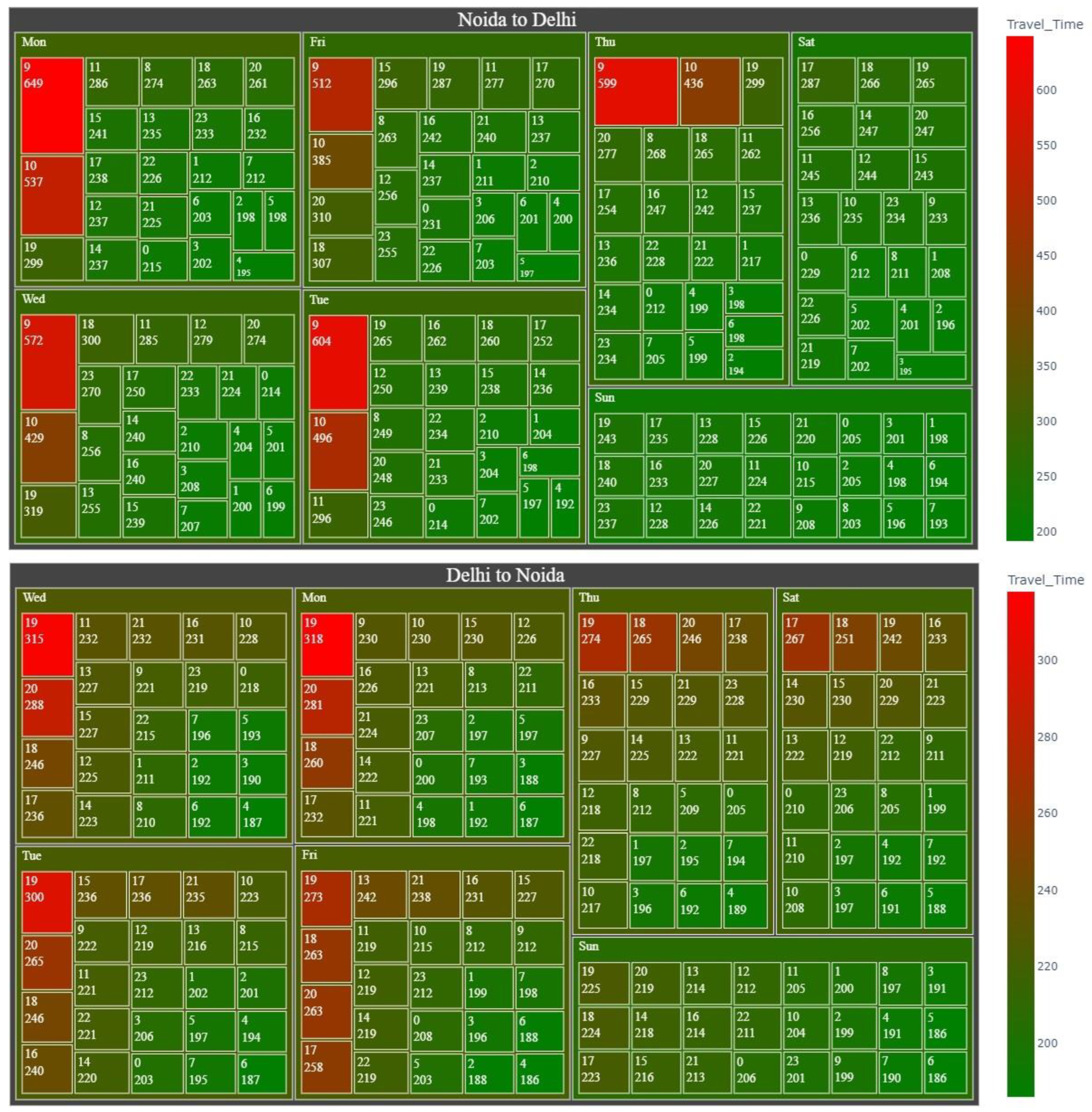
The daily analysis is performed to see the pattern of travel time variation with the day of the week. Initially, the trend/pattern in travel time variation is observed with the day of the week using a treemap. Figure 3 shows the treemaps that were plotted for both directions, Noida to Delhi and Delhi to Noida. From Figure 3 (treemap for travel direction Noida to Delhi), it can be observed that Monday is on the left topmost of the treemaps and red with an average travel time of 263 s. In contrast, Sunday is on the right bottom most of the treemaps and green in color, with an average journey time of 217 s. The week starting day Monday has a 21.2% longer travel time than the travel time on the off-day (Sunday). From the treemap, it is visible that weekdays have almost the same average travel time. The travel time on Saturdays is in-between the average travel time on working days (weekdays) and off-days (Sundays). In Delhi, some offices and businesses have a six-day working week while others have a five-day working week, so Saturday is a working day for some offices and businesses and an off-day for others. This difference in the number of working days could be the reason why Saturdays have an average travel time between the working days and Sundays.

A similar trend is also observed in the opposite direction, i.e., Delhi to Noida. On comparing the treemaps for both directions, it is observed that the effect of the weekend is more noticeable in the travel direction from Noida to Delhi.

3.2. Hourly Analysis

Hourly trend analysis is performed in addition to the daily analysis to determine the hourly pattern of travel time variation and identify the peak and off-peak times in the day.

Figure 4 shows the treemap for hourly analysis of the travel time variation. From the figure, it can be noticed that hourly travel time varies considerably from 186 s (On Friday 3 am to 4 am and Sunday 5 am to 7 am in the direction Delhi to Noida) to 649 s (On Monday 9 am to 10 am in travel direction Noida to Delhi). Also, the morning peak is visible from 9 am to 11 am for the travel direction of Noida to Delhi during the weekdays.

Figure 5 shows the heat map of the hourly travel time variation for different days of the week. During the weekdays, the morning peak is visible in the direction of Noida to Delhi, while in the travel direction of Delhi to Noida, the evening peak is visible. From this observation, it can be inferred that most of the trips are home-based work trips with home on the Noida side and work on the Delhi side. Also, from the heat maps, it can be observed that the peaks are present on the weekdays only. This observation further reinforces the earlier statement, i.e., most of the trips are home-based work trips.

In addition to the variation of the average hourly travel time with hour of the day and day of the week, it was also observed that the travel time varies noticeably even under free-flow (from 78 s to 497 s) and traffic jam conditions. These noticeable variations hint towards the common issues of heterogeneity and disorderliness in developing countries.

4. Methodology

The trends of travel time variation that were obtained from the analysis in the previous section are used to develop the travel time prediction model. First, a historical trajectory database is built using the steps that are explained in the pre-processing data section to develop travel time prediction models. Next, data outliers are removed from the travel time data that were obtained in the data pre-processing step, as described in the data outliers removal section. Finally, the data are aggregated hourly to further minimize the effect of remaining local outliers. The present study uses the last four weeks’ data as the test dataset and the remaining data as the training dataset. The models are developed using the training dataset and tested on the test dataset.

Figure 6 shows the flowchart of the overall methodology that was proposed for developing the travel time prediction models.

4.1. Historical Average Method

In this method, model development starts with building the historical trajectory database and then searching for the matched trips. From the data analysis in the previous section, it is observed that the travel time in the study segment depends upon the hour of the day, day of the week, and direction of the travel. So, these are used as matching criteria for searching the matched trips. Fixed interval search (FIS) and the k-nearest neighbor (KNN) method are generally used to match the trip departure time. In the present study, fixed interval search (FIS) is used for matching the trips. The procedure for comparing and finding the matched trips is as follows:

(1)

Find the trips whose direction of travel is the same as specified by the users and add these trips to the subset J_S_S.

(2)

Apply fixed interval search to J_S_S and the departure time that is specified by the user Td to find the matching trips, which are then saved in the resulting set J_S_M.

To predict the travel time using the traditional historical average method, trips in J_S_M shall follow the normal distribution. The three most common forms of normal distribution tests that are used in the literature are graphic, empirical, and normality test methods. The present study uses the empirical method as a normal distribution test. The ratio of sample median to the arithmetic mean (denoted by r_mm) and arithmetic mean to standard deviation (expressed by r_md) is used to evaluate the distribution of matched trips. The sample data follow a normal distribution when r_mm is greater than 0.9 but less than 1.1, and r_md is greater than 3 [39].

Finally, the travel time is predicted using the mean value approach. According to the mean value approach, the arithmetic means of the matched trip’s travel time data gives the predicted travel time if the matched trip’s travel time follows the normal distribution.

4.2. Linear Regression Method

The linear regression method is one of the most basic and widely used machine learning algorithms for predictive analysis. This method shows a linear relationship between a dependent and one or more independent variables. It determines how the value of the dependent variable changes due to the value of the independent variable. The model in the present study is fitted using the linear regression submodule of the sci-kit learn machine learning package’s linear model module. The present study used the day of the week and the hour of the day as independent variables and travel time as the dependent variable.

4.3. Decision Tree

The decision tree is one of the most powerful and popular machine learning algorithms falling under supervised learning. The decision tree algorithm builds a training model that can predict the target variable’s value by learning simple decision rules from the training data. In the present study, the decision tree algorithm is implemented using the decision tree regressor modules of the sci-kit learn machine learning package. The present study used a decision tree to predict the travel time (target variable) based on the hour of the day and the day of the week. The model is trained with a maximum depth of tree as 10 using the best splitter and squared error as the criterion for decision.

4.4. Random Forest

Random forest constructs many decision trees before combining them to produce a more accurate and consistent prediction. In the present study, the random forest algorithm is implemented using the random forest regressor module of the sci-kit learn machine learning package. The random forest model for the present study is trained using 100 trees in the forest using squared error criteria to predict the travel time based on the hour of the day and the day of the week as features. While training the model, the parameter max_features is set to auto to consider all the features while looking for the best split. In the present study, the whole training dataset is used to build each tree in the random forest.

4.5. Gradient Boosting Regressor

The concept of boosting came from the idea of whether a poor learner could be modified to become a better learner. Gradient boosting creates a prediction model from a collection of weak prediction models, most commonly decision trees. For developing the gradient boosting model in the present study, the gradient boosting regressor module of the sci-kit learn ensembles package is used. Gradient boosting regressor builds an additive model forward stage-wise fashion and uses squared error as a loss function and decision tree as a weak leaner. The GBR model in the present study performs 100 boosting stages and uses all input features (the hour of the day and the day of the week) with a learning rate of 0.1. The current research optimizes both tree-specific and boosting parameters to obtain the best performance without much reduction in computation speed.

To get the maximum accuracy, hyper parameters were optimized such that the model gives maximum accuracy without underfitting or overfitting to the training dataset. To avoid underfitting and overfitting, bias, as well as variance, was minimized.

Table 5. Errors of the training and testing datasets.

Direction of Travel		LM	DT	RF	GBR
Noida to Delhi	Training	15.01	13.35	12.25	12.26
	Testing	14.69	12.59	11.23	11.32
Delhi to Noida	Training	8.08	8.56	7.97	7.90
	Testing	9.49	8.53	7.55	7.41

shows the error on the training and test datasets for the four machine learning methods that were considered in the present study. From the Table 5, it is clear that the models that were considered in the study are neither underfitted nor overfitted.

5. Results and Discussion

This section of the paper shows the prediction results and evaluates the performance of the various travel time prediction models that were developed in the present study. Figure 7 compares the actual travel time with the travel time that was predicted by the models that were developed in the study over the test dataset.

From Figure 7a, it can be observed that the horizontal average method smoothens out the peaks due to recurring rush hours and is unable to reproduce the actual travel time pattern. The linear regression model cannot learn about the absence of peaks on Saturday and Sunday. The decision tree can learn that weekends do not have the peak but cannot learn minor patterns, especially when the travel time is less than average. Random forest and gradient boosting regressor can learn the pattern best.

Conclusions in the above paragraph are also supported by the observation from Figure 7b, showing the actual travel time and travel time that was predicted in the direction of Delhi to Noida by models that were developed in the study.

5.1. Performance Evaluation Using MAPE

Models that were developed in the current study can be evaluated using various criteria such as model accuracy, simplicity, suitability, and transferability criteria. As the present research develops models for the traveler information system that have inherent requirements of simplicity, all the models that were selected in the study are already chosen by considering the simplicity and suitability criteria. Studying the transferability of the results is beyond the scope of the present study. Hence, the models are evaluated using accuracy only. The MAE (mean absolute error), MSE (mean square error), RMSE (root-mean-square error), and MAPE (mean absolute percentage error) are generally used to quantify the errors that are produced by the prediction models.

The mean absolute percentage error is one of the most commonly used key performance indicators (KPIs) to measure forecast accuracy and is used in the present study. The following formula gives it:

$$\mathrm{MAPE}=\frac{1}{\mathrm{N}}\times {\sum }_{\mathrm{i}=1}^{\mathrm{N}}\frac{\left|{\mathrm{PTT}}_{\mathrm{i}}-{\mathrm{ATT}}_{\mathrm{i}}\right|}{{\mathrm{ATT}}_{\mathrm{i}}}\times 100, \mathrm{i}=1,2,\dots ,\mathrm{N}$$

(1)

where N = number of trips to be tested, PTT_i = the travel time that is predicted for the ith trip, and ATT_i = the actual travel time that was measured of the ith trip,

Table 6. Comparison of performance using MAPE (%).

Direction of Travel	Day Classification	HA	LM	DT	RF	GBR
Noida to Delhi	Weekdays	15.90	14.44 (−1.46)	12.4 (−3.5)	11.29 (−4.61)	11.33 (−4.57)
	Saturday	19.53	16.70 (−2.83)	15.34 (−4.19)	13.51 (−6.02)	12.6 (−6.93)
	Sunday	13.63	13.94 (0.31)	10.79 (−2.84)	8.62 (−5.01)	9.96 (−3.67)
	All Days	16.09	14.69 (−1.4)	12.59 (−3.5)	11.23 (−4.86)	11.32 (−4.77)
Delhi to Noida	Weekdays	12.12	9.66 (−2.46)	9.05 (−3.07)	7.98 (−4.14)	7.75 (−4.37)
	Saturday	9.26	9.33 (0.07)	7.4 (−1.86)	6.85 (−2.41)	7.14 (−2.12)
	Sunday	7.26	8.8 (1.54)	7.07 (−0.19)	6.09 (−1.17)	6.01 (−1.25)
	All Days	11.02	9.49 (−1.53)	8.53 (−2.49)	7.55 (−3.47)	7.41 (−3.61)

compares and shows variations in the performance of all the travel time prediction models with the direction of travel, day classification, and travel time on the road segment. For analyzing the performance variation, weekdays are classified into the working day, Saturday, and Sunday. Saturday and Sunday are not combined because most trips to the study area are work trips, and usually, Sunday is an off-day, but Saturday is a working day for some offices and businesses and an off-day for others. Values in the bracket are the percentage difference in the MAPE values of machine learning methods w.r.t. to the baseline method (historical average method).

From Table 6, it can be observed that all the methods perform better in the direction Delhi to Noida as compared to Noida to Delhi as traffic in this direction has mostly return work trips which are distributed over a more extended period of time, usually from 4 pm to 9 pm on weekdays while the direction Noda to Delhi has a concentrated morning peak due to work trips that are distributed over a short period, usually 9 am to 11 am on weekdays.

From Table 6, it can also be observed that methods perform best on Sunday because of the absence of congestion and noticeable peak hours.

For travel direction, Noida to Delhi performance on Saturdays is the worst because of the no lane discipline. Under extreme congestion and free-flow conditions, the effect of the lane discipline is not noticeable. But, when the congestion is in-between, no lane discipline causes significant vehicle–vehicle variability, which leads to poor performance of the travel time prediction models. For the travel direction from Delhi to Noida, the performance on Saturday is in-between the performance on weekdays and Sunday.

For comparison among the algorithms, the historical average method performs the worst. RF and GBR perform almost equally well and are the best among the five methods that were considered in the present study.

The complete evaluation procedure for the travel time prediction model for traveler information system examines the distribution of error instead of relying solely on the mean value. So, if error measurement statistics are calculated separately for different periods, then the evaluation of the model can be improved. Figure 8 shows the error distribution of all five models that were used in the study. From Figure 8, it can be observed that all the methods perform poorly during peak hours (rush hours) because of the vehicle–vehicle variability due to no lane discipline and heterogeneous traffic.

5.2. Performance Evaluation Using Satisfaction Rate

The satisfaction rate (SR) can also be used for the performance evaluation of the travel time prediction models, mainly when the predicted travel time is used for the traveler information system. It is defined as the percentage of trips for which the estimation error is less than 25%. It is calculated using the following equation:

$$\mathrm{SR}=\frac{{ \mathrm{N}}_{\mathrm{S}}}{{\mathrm{N}}_{\mathrm{T}}}\times 100$$

(2)

where, N_s = the number of trips having an absolute percentage estimation error less than 25%, N_T = the total number of trips

Table 7. Comparison of performance using the satisfaction rate.

Direction of Travel	Day Classification	HA	LM	DT	RF	GBR
Noida to Delhi	Weekdays	79.79	86.46	85.83	86.67	88.75
	Saturday	88.54	87.50	93.75	96.88	95.83
	Sunday	91.67	88.54	95.83	96.88	96.88
	All Days	82.74	87.50	88.39	89.58	90.92
Delhi to Noida	Weekdays	90.42	92.84	94.58	95.63	95.83
	Saturday	96.88	93.08	98.96	98.96	98.96
	Sunday	98.95	93.92	98.95	98.95	98.95
	All Days	92.55	93.17	95.83	96.57	96.72

shows the comparison of the performance of all the methods using the satisfaction rate.

The results in Table 7 agree with the comparison in terms of MAPE in Table 6, with one exception as mentioned below.

In terms of the satisfaction rate, all the models perform better on Saturdays than on weekdays in both travel directions. This observation further reinforces the earlier conclusion that lane indiscipline causes poor prediction of all the algorithms on Saturdays in the travel direction Noida to Delhi. Lane indiscipline causes abrupt changes in the travel time and hence produces an enormous error value, but the instances of lane indiscipline are lesser in number. So, Saturdays have better performance than weekdays in terms of satisfaction rate, which is the average number of trips having an error of more than 25%.

The present study results are slightly lagging behind similar studies that were done in advanced countries such as the USA [13,40], possibly due to high random variability that was introduced because of the heterogeneous nature of the traffic and disorderly movement of vehicles that are observed in Indian conditions. However, the results are superior to the results of studies that were done in traffic conditions similar to the current research possibly because of the inclusion of data of almost all types of vehicles that are present in the stream and all traffic conditions by taking the data continuously for almost one year. For example, the present study’s results are superior to a study that was done in China [22]. The random forest method [22] predicted the travel time for open-pit trucks on temporary roads and fixed roads with a MAPE value of 20.7 and 21.7, respectively, when no meteorological features were considered.

The results of the present studies are significantly better than that of Kumar et al. [31,33], which used a GPS trajectory dataset of metropolitan transport corporation buses. The present study results are better than those using data from more reliable sources such as Bluetooth sensors [36] and cameras [35]. The present study produced results that are comparable to the results of the hybrid data fusion method in Anusha et al. [32] using data from VISSIM, cameras, and GPS.

Vasantha Kumar & Vanajakshi [34] collected GPS trajectory by manually carrying GPS devices in three categories of personal vehicles (Two-heeler, three-wheeler, and cars) in addition to GPS trajectory that was collected by Metropolitan Transport Corporation (MTC) buses. This additional information about the vehicle category improved the travel time prediction accuracy, but the accuracy of the present study using a massive GPS dataset is better than that of the Vasantha Kumar and Vanajakshi [34].

The discussion shows that the GPS trajectory dataset is an excellent alternative data source for travel time prediction in Indian traffic conditions when used with modern machine learning algorithms.

Table 8. Comparison of the efficiency using the processing time (seconds).

Direction of Travel	LM	DT	RF	GBR
Noida to Delhi	0.027	0.059	4.094	1.620
Delhi to Noida	0.019	0.050	3.700	1.478

shows the comparison of models that were used in the study based on the processing time, i.e., the time that is required to fit the model to the data. This comparison shows that the linear model has the least processing time, whereas the random forest has the highest processing time. However, based on both performance and computational efficiency, GBR is the best model to predict travel time in Indian traffic conditions.

6. Conclusions

In this article, the problem of travel time prediction on a corridor of an Indian expressway using historical GPS trajectories of probe vehicles is studied. This study explores the possibility of using the GPS trajectory dataset for travel time prediction and the ways to improve the accuracy of travel time prediction in Indian traffic conditions having heterogeneous disordered traffic. The study also investigates the improvement in travel time prediction accuracy by replacing the classical historical average method with modern machine learning algorithms.

First, a GPS trajectory dataset of around 2000 probe vehicles consisting of almost all types of vehicles that are present in traffic running in India’s Delhi—NCR region and installed with manufactured GPS devices is collected. Then, the pattern analysis of travel time data is carried out after obtaining travel time data from the GPS trajectory dataset and removing the outliers having a travel time value more than the walking time. Temporal and spatial analysis is done for various hours of the day, days of the week, and the direction of the travel.

Next, travel time prediction models are trained and tested using the training and test dataset. The predicted values are compared with the observed travel time values for testing the models. The prediction accuracy of the models is compared using MAPE and SR as measures.

The results show that the historical GPS trajectory dataset of probe vehicle consisting of all types of vehicles that are present in the stream serves as an excellent alternative data source for travel time predictions in heterogeneous disordered traffic conditions. The use of a large dataset that is collected over a long continuous period of time covering all types of traffic conditions, with high temporal and spatial resolution improves the travel time prediction accuracy and gives competitive results despite being hampered by high random variability due to heterogeneity and disorderliness. The inclusion of all types of vehicles that are present in the stream make the better representation of the real-world dynamics and gives robust and reliable predictions. The inclusion of all types of vehicles that are present in the traffic streams also provided new insights that heterogeneity and disorderliness that introduces high random variability in travel time. The results of the present study show that using a GPS trajectory dataset can predict the travel time more accurately than the travel time using reliable data sources such as cameras, Bluetooth sensors, etc., even in Indian traffic conditions.

Performance and efficiency comparison results of the present study can also be used as a guideline for selecting the appropriate prediction algorithm for various situations. For selecting the best method for travel time prediction, it can be concluded that random forest and gradient boosting machine learning algorithms perform equally well and are better than the traditional historical average method and the basic machine learning algorithms (decision tree and linear regression). However, the gradient boosting regressor is more efficient than the random forest. So, if the computational efficiency is also taken into account, then gradient boosting regressor is the best method to predict the travel time in heterogeneous disordered traffic conditions. The present study also concludes that improving the performance of the model/algorithm during rush hours can result in further improvement in the accuracy of travel time prediction. The performance during rush hours can be improved by incorporating additional data such as the type of vehicle, vehicular characteristics (top speed, maximum acceleration), weather conditions, incidents, etc. This conclusion is also supported by the study that was conducted by Qiao et al. [41], which showed that weather information helps to improve the travel time prediction as adverse weather usually increases the travel time.

The present study recommends a novel combination of GPS trajectory dataset and modern machine learning algorithms (random forest and gradient boosting algorithms) that are proposed in the study to predict the travel time that is required for the development of traveler information systems in developing countries such as India, Pakistan, Nepal, Bhutan, Bangladesh, Sri Lanka, etc., because of the ability to predict travel accurately time with minimum investment.

The present study has the limitation of predicting only one travel time for all the vehicles in a traffic stream. In the future, a separate travel time prediction model based on vehicle categories can be developed for different vehicle types. The performance of the travel time prediction models that are proposed in the current study can be further improved by using the separate model for the short-term and long-term predictions and then combining by using an interaction term. Also, different models corresponding to different weekdays combined with the help of interaction terms can also be attempted in the future to improve the performance, especially during rush hours.