Article

Energy Consumption Analysis Using Measured Data from a Net-Zero Energy Commercial Building in a Cold and Dry Climate

1
Department of Building Research, Korea Institute of Civil Engineering and Building Technology, Goyang 10223, Korea
2
Mechanical and Biomedical Engineering, Boise State University, 1910 University Drive, Boise, ID 83725, USA
*
Author to whom correspondence should be addressed.
Sustainability 2022, 14(16), 10346; https://doi.org/10.3390/su141610346
Submission received: 4 May 2022 / Revised: 10 August 2022 / Accepted: 18 August 2022 / Published: 19 August 2022

Abstract

:
Zero-energy buildings have a critical role in reducing global energy use and greenhouse gas emissions. However, few studies have analyzed net-zero energy commercial buildings using measured energy use such as whole-building level and end-use level data. This paper presents an energy consumption analysis for the first net-zero energy commercial building in Idaho, U.S., in a cold and dry climate using measured end-use data from this building as well as measured whole-building energy use. Monthly bill data analysis, end-use data analysis, and Energy Use Intensity (EUI) analysis were conducted. The combined analysis of this study shows that the HVAC system was the most sensitive to the outside air temperature, showing different energy use percentages of 48.4%, 35.1% (the heating period), 21.6% (the weather-independent period), and 33.4% (the cooling period), respectively. Lighting had the highest percentage of 35.2% for the weather-independent period. The PV electricity generation was higher than the building electricity use, except from December 2017 to February 2018, and the building was net-positive from an energy perspective. The calculated EUI of the building was 34.2 kWh/m2·y, which can be compared to the EUIs of other net zero energy buildings. The approaches developed in this study can be useful for analyzing several net zero buildings by different weather profiles.

1. Introduction

Net zero energy buildings (nZEBs) have a critical role in reducing energy use and greenhouse gas emissions [1,2]. Advanced technologies for energy consumption reductions, as well as indoor environmental quality improvements, have been applied to nZEBs [1]. Solar, geothermal, bioenergy, and/or wind (i.e., renewable energy) are also significant in meeting buildings’ energy demand from nZEBs. The U.S. has targeted to make all commercial buildings become nZEBs by 2050 [3,4]. The EU has required all new buildings to become zero-emission buildings from 2030 [5]. Thus, life cycle assessment and life cycle cost analysis are also important to implement advanced technologies for the nZEB design and to consider their overall environmental and economic impact [6,7]. Moreover, in order to provide a holistic approach to nZEBs, Torcellini et al. defined nZEBs using the four factors site energy, source energy, energy cost, and energy emissions [8]. Several nZEB projects were already conducted in various nations, and the projects were well-studied [9].
Thus, accordingly, there are several approaches [2] to analyze nZEBs, such as energy analysis (e.g., primary energy site energy, end-use energy, etc.), emission analysis, and cost analysis. Most of the previous studies have used simulation [7,10,11,12,13,14,15,16,17], measured data [18], and both simulation/measured data [19,20,21,22] analysis to analyze nZEBs.
Due to the attribute of simulations, the simulation-based studies focused on the design and/or estimation of various energy systems to achieve nZEBs. Kim et al. [7] analyzed the life-cycle cost of a zero energy office equipped with a grid-connected photovoltaic (PV) system and an air-source variable refrigerant flow (VRF) heat pump system. A prototype building model obtained from EnergyPlus was used for simulations in 15 US climate zones. The initial investment costs of PV and VRF systems, annual operation costs, maintenance costs, and PV investment incentives were considered for the simulation-based life-cycle cost analysis. Their results showed that the life-cycle costs for nZEBs were significantly lower in the hot and mild climate zones.
Aksamija [10] estimated the multiple designs of material selection, building envelope, HVAC and lighting systems, occupancy loads, and renewable energy applications for existing buildings to achieve zero energy goals. The researcher used a case-study commercial building located in Massachusetts, the U.S. Various simulations were conducted using eQuest modeling with adaptive reuse and retrofits from passive design strategies. The final results achieved net-zero energy use with effective design approaches and various renewable energy such as solar, wind, hydro, and biomass energy.
Fadejev et al. [11] investigated the performance of several ground heat exchangers and thermal storage options for a ground-source heat pump plant. The IDA-ICE simulation models were used to study a commercial hall-type nZEB, which was located in Hämeenlinna, Finland, in a cold climate. Energy piles, vertical boreholes, and solar thermal storage with/without exhaust air heat were specifically estimated to find advantageous options for the nZEB design using the simulations. Their results showed that the ground-source heat pump plant was more efficient at 15% than the district heating plant. In addition, the solar thermal storage with exhaust air heat reduced the energy piles field length by 2.6 times.
Simulation-based studies for nZEBs even covered smart buildings and smart grids. AlFaris et al. [12] studied the impact of intelligent systems such as the Internet of Things (IoTs), Home Energy Management System (HEMS), and Smart Meters (SM) in residential buildings. Using eQuest simulations, they evaluated a case study, a family villa smart home in Riyadh in Saudi Arabia, in the hot climate. An annual energy performance improvement (i.e., Energy Use Intensity (EUI)) was estimated at 37% using smart technologies.
Tumminia et al. [13] investigated an optimal grid interaction (i.e., smart grid) for minimum greenhouse gas emissions from nZEBs. They used a residential prototype of nZEB located in Messina, Italy. Using the TRNSYS simulation environment, a multidisciplinary design approach was proposed considering PV, fuel cell, and energy storage systems. They suggested a holistic approach considering various sustainable aspects to implement nZEBs into the smart grids.
Other simulation-based studies estimated an advanced renewable energy system [14], an energy storage system [15], electric vehicles [16], and even hydrogen vehicles [16,17] for nZEBs in the smart grid environment. Shaterabadi et al. [14] investigated a new advanced wind turbine, called INVELOX, for the nZEB design to achieve plus-ZEBs that lower cost and pollution. A solar water heater with PV systems, air-to-water heat pump, ventilation, micro-combined heat and power (CHP), and energy storage systems were also considered. Mixed-integer linear programming and the Epsilon constraint method with the fuzzy satisfying approach were used to suggest multi-objective energy management. The wind speed and solar radiation, which were measured in Kermanshah city, Iran, were used to make reliable simulation results. When the pollution priority was considered, the multi-objective energy management reduced the total cost and pollution by 28.7% and 54.7%, respectively, and reached almost a plus-ZEB with surplus power to the grid.
Luo et al. [15] developed a new concept of the PV-thermoelectric-battery wall system with the “double zero” approach. The “first zero” indicated zero heating and cooling loads through walls in buildings, and the “second zero” indicated net-zero energy use to achieve the “first zero”. Using the Model-based Predictive Control (MPC) approach to optimize the PV-thermoelectric-battery wall system, nZEBs were estimated in different climate zones, such as cold, mixed, and hot zones, in China. Based on the MPC simulation results, it was found that the energy storage (i.e., battery) capacity and operation period for the new system was important.
Cao [16] estimated electric and hydrogen vehicles for the integration into nZEBs. Wind and solar energy were also considered using the TRNSYS simulation for the Helsinki metropolitan region, Finland, in the humid continental climate. The results showed that the efficiency of electric vehicles was more helpful than the efficiency of hydrogen vehicles in meeting the balance for nZEBs. Cao et al. [17] investigated nZEBs with hydrogen vehicles in the Finnish and German climates using the TRNSYS simulation as well. Wind energy was more beneficial to nZEBs in the Finnish climate, but solar energy was preferred in the German climate.
While all the previous simulation-based studies were conducted to estimate various potential aspects of energy systems for nZEBs, one study was only found for measured data-based studies. Doherty and Trenbath [18] analyzed plug loads using device-level consumption obtained from a submeter of Ibis IntelisocketTM in a case-study office (research facility) located at the National Renewable Energy Laboratory (NREL) in Golden, Colorado in the U.S. They developed a disaggregated model using a device inventory and using few sub-metered data. They found that their model can represent plug load profiles using the data during three months, which can help occupants better understand their plug loads for energy efficiency. However, their model was not able to accurately identify the total amplitude of the sub-metered data.
The studies using both simulation-based and measured data-based approaches were also conducted for nZEBs [19,20,21,22]. Zhou et al. [19] compared measured operational energy use during two years with simulated design energy use to investigate the energy performance of nZEBs. To analyze measured energy use, they used a case-study office building located in Tianjin, China. The eQuest building energy model was used to estimate energy use at the design phase. They found that the actual building operation was different from the building operation intended at the design phase. The difference should be investigated in detail to achieve actual nZEB.
Wu et al. [20] estimated the HVAC options of ventilation, heat pump, and dehumidification for residential nZEBs. The case-study net-zero energy residential test facility (NZERTF) was located in Gaithersburg, Maryland, in the U.S. A validated model of TRNSYS, which was calibrated with monthly measured data, was used to calculate energy, comfort, and economics regarding the HVAC options. They found that practical payback periods were obtained when an air-source heat pump (ASHP) with an energy recovery ventilator and dedicated dehumidification was used for the residential nZEB.
Suh and Kim [21] analyzed nZEBs to observe the impact of passive and active design approaches with renewable energy such as PV, solar thermal, and geothermal heat pump systems. Monthly measured electricity and gas use from four community buildings located in Incheon, South Korea, were used to calibrate a building energy simulation model from DesignBuilder. After the calibration, the model was used to identify the best solution for nZEB. Even though the passive and active design approaches helped lower heating, cooling, and lighting energy use, domestic hot water energy use was large. The results from the calibrated simulation model suggested that the PV system using additional modules and the geothermal system was the best option.
Shin et al. [22] compared the results from measured energy savings and estimated energy savings using change-point linear regression and calibrated simulation models. Using a case-study office located in Texas, a side-by-side comparison was conducted between un-renovated and renovated spaces. They found that the renovated space with a VRF system, high-performance insulation, lighting with occupancy detection, and thermostats with occupancy detection achieved 37–40% energy savings compared to the un-renovated space.
In summary, the various studies based on simulation, measured data, and both simulation/measured data have been conducted for nZEBs in several climate conditions. However, even though the previous studies have covered many energy systems applied to nZEBs and their energy use, no studies have analyzed nZEBs using both measured whole-building level and end-use level data. In addition, the previous studies did not conduct weather-sensitive analysis for their end-use level energy use data. They did not also provide effective data management for the big end-use data processing from HEMS or Building Energy Management System (BEMS) in nZEBs. Thus, in this paper, combined energy performance analysis using measured data was conducted with three different approaches: utility billing data analysis, end-use data analysis, and Energy Use Intensity (EUI) analysis. The purpose of this paper is to effectively use available measured energy use data for better analyzing the building energy performance. The combined energy analysis and results of this paper can provide the information to better identify energy use patterns by weather and by time. The first commercial nZEB located in a cold and dry climate [23] was used for the analysis using measured whole-building energy use and end-use data. The calculated EUI of the nZEB was 34.2 kWh/m2·y, which can be compared to the EUIs of other nZEBs in different climates.
In the second section, the nZEB used for this paper was introduced, and the three analysis approaches were explained. In the third section, results from the three analysis approaches were summarized and discussed. In the final sections, the findings and conclusions of this paper were described, respectively.

2. Materials and Methods

In this paper, three analysis approaches were conducted for the first net-zero energy commercial building in Idaho, the U.S, as shown in Figure 1. This Twenty Mile South Farm (TMSF) Administration and Maintenance Facility, operated by the City of Boise in Idaho, was built to help manage bio solids produced as part of the wastewater treatment process at the two treatment facilities [24]. Boise is categorized in the cold and dry climate as 6B [25]. Winters are not freezing cold, but summers are arid. It shows the lowest monthly average daily temperature of −0.7 °C and the highest of 27.6 °C during the period used in this study.
The farm comprises 17.1 km2 and is located approximately 32 km (20 miles) south of Boise. This facility was designed as Idaho’s first commercial net-zero energy building, and it received the LEED GOLD certification [26]. The final occupancy took place August 2016. This facility is one story building with a mezzanine floor, which consist of an office building (636 m2), mechanic shop (459 m2), and maintenance shop and parts warehouse (280 m2) with a total gross area of 1375 m2. The building features a high-performance envelope, ground source heat pumps (HPs), and a 24 kW(DC) PV array on the south-facing roof. The detailed information about the building is shown in Table 1. The parameters in the table were retrieved from the drawings. The following subsections summarize each analysis of the three approaches for the first nZEB in Idaho.

2.1. Monthly Bill Data Analysis

Figure 2 shows the procedures used for the monthly bill data analysis. First, monthly utility bill data from September 2017 to August 2018 and corresponding outside air temperature data from the National Oceanic and Atmospheric Administration (NOAA) site [27] at the Boise airport (approximately 12 miles NNW of the facility) were collected. The monthly utility bills included the electricity use of the facility and the electricity generation from the PV system by billing period. Second, the data were organized by monthly average daily period to normalize the different number of days for each month. Third, the time-series analysis was conducted to observe the energy trends of electricity use, electricity generation, and net electricity use. Finally, the change-point linear regression analysis [28,29] was conducted to find the building energy signature, which examines the sensitivity of the energy consumption to outside air temperature.
In this paper, Equation (1) of the five-parameter (5P) change-point linear model was used for the change-point linear regression analysis [29,30,31]. The 5P model is typically appropriate because all the energy source of the nZEB facility is electricity.
E t o t   =   E w . i .   +   H S ( T O A     T h . b . )   +   C S ( T O A     T c . b . ) +
where E t o t is the whole-building energy use,   T O A is the outside air temperature, E w . i . is the weather-independent energy use, H S is the heating energy use against the outside air temperature, T h . b . is the heating balance-point temperature indicating the onset of heating-related energy use, C S is the cooling energy use against the outside air temperature, T c . b . is the cooling balance-point temperature indicating the onset of cooling-related energy use, and (   ) and (   ) + are the notations that the values of the parentheses shall be zero when they are positive and negative, respectively.
The coefficients of the 5P change-point linear model can be interpreted, especially when the coefficients are changed during two different periods. Basically, this statistical model is the black-box, data-driven method, but this model can be the gray-box method [32] because the coefficients are interpretable, and the interpretation was verified in the previous studies [28,33]. For example, H S varies by heating load (i.e., conductive heat loss through building envelope and convective heat loss through infiltration and ventilation) and heating system efficiency. In addition, T h . b . is the heating balance-point temperature that begins heating space conditioning. This coefficient varies by heating setpoint, internal heat gain, and heating load [33]. In order to interpret the coefficients more specifically, the forward methods are required [34,35,36,37].
For the indices of the goodness-of-fit and accuracy for the 5P model, the coefficient of determination (R2) and Coefficient of Variation of the Root-Mean-Square Error (CV-RMSE) were used (see Equations (2) and (3)). The 5P model can be evaluated using higher R2 and lower CV-RMSE to see how well the model fits measured data. CV-RMSE was used in this study because the metric can show the performance of a model rather than the variability and difference of the data shown in RMSE [38].
R 2   =   i ( y i     y ¯ ) 2     i ( y i     y ^ i ) 2 i ( y i     y ¯ ) 2
CV     RMSE   =   i ( y i     y ^ i ) 2 n     p y ¯ × 100   %
Here, y i is energy use from the monthly average daily bill data or energy use from the daily end-use data, y ^ i is energy use predicted by the change-point model, y ¯ is the average of energy use data from the monthly average daily bill data or the average of energy use from the daily end-use data, n is the number of energy use data points, and p is the number of parameters.

2.2. End-Use Data Analysis

Figure 3 shows the procedures for the end-use data analysis. Each individual circuit breaker in the building is equipped with a power logger that reports to a central server. A total of 254 circuits are logged, and the results for the first 10 months of 2018 were provided in the form of 254 CSV files. Each file contained a time log consisting of a time stamp and cumulative kWh for a period of time at 10 min intervals. In general, each log started and stopped at different times. In order to make use of the data, significant processing had to be performed.
First, to find a common time interval, a Python script was written to read each file and record the starting time, the ending time, and the delta kWh of each file. It was found that a large number of files had zero, or nearly zero (≤0.001), electricity consumption and were hence excluded from further analysis. There were 180 files with non-zero consumption measured. The longest common time span for those files started 12 February 2018 and ended 3 October 2018. Within that time frame, it was found that there was a gap in the data from 8 June to 20 June.
By using the second Python script, the electricity use data from the 180 circuits was validated by comparing the total to monthly utility bills. It was assumed that the data from the 180 circuits represented all the electricity use for the TMSF facility. The data gap from 8 June to 20 June spanned two billing periods, so those bills were not able to be verified. Table 2 below shows the results from the validation process. The results from the validation process showed close enough to capture much of the energy use of the facility within ±2.0% differences from the electricity bills.
Finally, to analyze breakdown of the end-use from the various circuits, the third Python script was used to create a master spreadsheet that cataloged each circuit and calculated the change in kWh over the bill periods. Then, building zones and end-use types of each circuit data were categorized based on the building plans and information from the building manager and occupants.
The following building zones were identified:
  • Office
  • Mechanic Shop
  • Maintenance Shop and Parts Warehouse
  • IT (mezzanine IT room)
  • All (those circuits that span building zone areas or support the entire building)
  • The following end-use types were also identified:
  • Systems (e.g., gates, control system dashboard, gates, irrigation, fire suppression)
  • HVAC
  • Lighting
  • Plug Loads
  • Appliances
  • Machinery
  • Domestic Hot Water (DHW) System
Table 3 shows an example of this process. For the zone categorization, the “All” tag was used if the circuit was deemed to support the entire facility or was outdoors (e.g., outdoor lighting, fire suppression, irrigation). Similarly, for the end-use categorization, the “Systems” code was used to capture miscellaneous loads such as the security gates, control system dashboard, irrigation, and fire suppression.
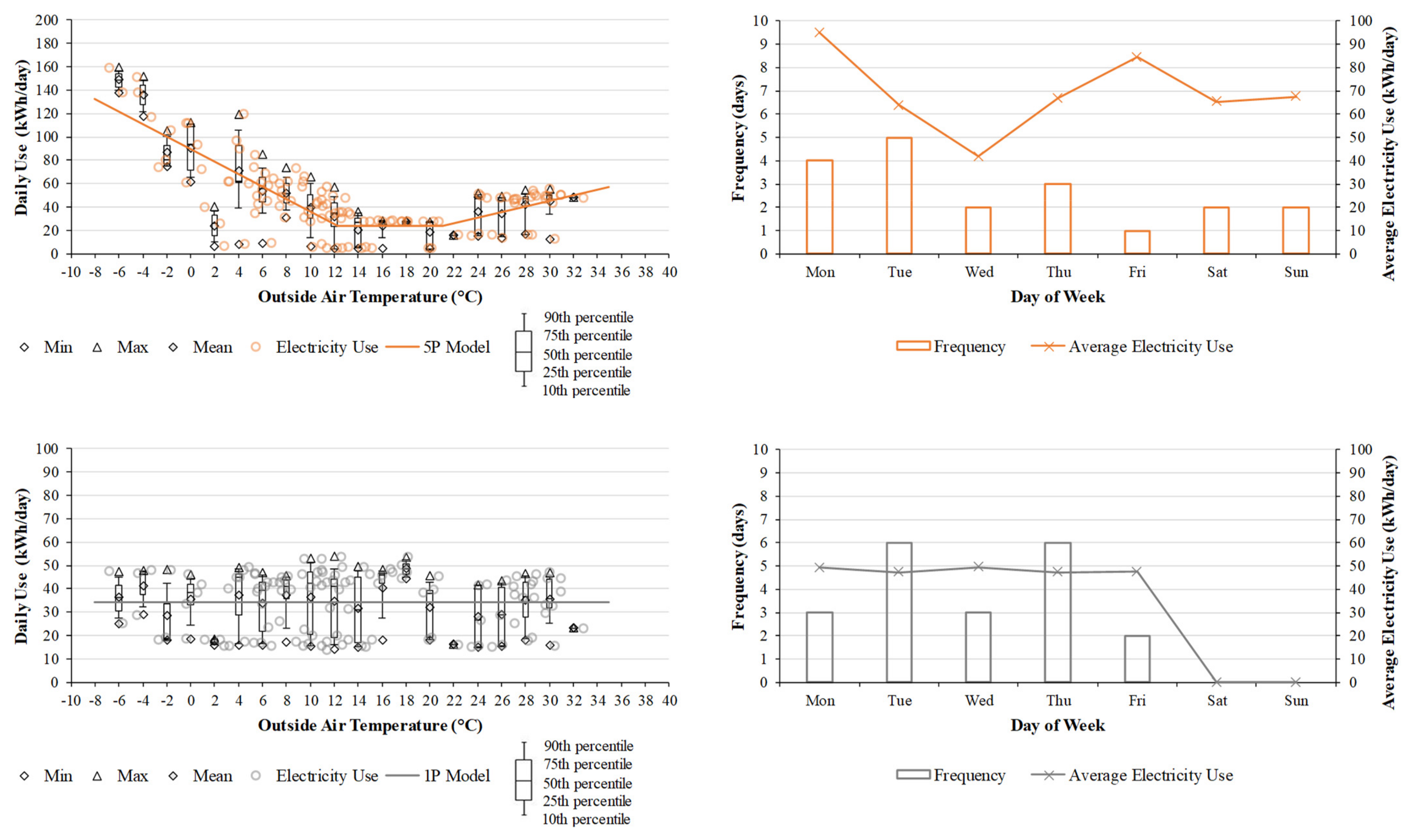
By using the process of the end-use data analysis, daily interval data were also managed. Using the daily interval data of the end-use type during the bill periods of March, April, May, and August, the change-point linear regression analysis (see Equation (1)) was conducted to observe the weather sensitivity for each end-use level energy use data. For some of the end use categories, the one parameter (1P) mean model [29] was found to be appropriate because there was no sensitivity to outside temperature (e.g., lighting, plug loads, appliances, machinery, DHW systems, etc.). Other categories (e.g., HVAC) showed strong sensitivity, so traditional change-point models were found to describe the dependency. To check the accuracy of the 1P model, Coefficient of Variation of the Standard Deviation (CV-SD) was used (see Equation (4) below). Lower CV-SD indicates how well the model fits the daily end-use data.
CV     SD   =   i ( y i     y ¯ ) 2 n     1 y ¯ × 100   %
Here, y i is energy use from the daily end-use data, y ¯ is the average of energy use data from the daily end-use data, and n is the number of energy use data points.
Finally, using the advanced quartile analysis [39], day of the week patterns were also identified. In this paper, high energy use above the 90th percentile on 2.0 °C bins were analyzed to find which day had the high energy use by each end-use type.

2.3. EUI Analysis

The EUI analysis was also conducted in this paper. The sum of the measured end-use level data from the 180 circuits was used. The data examined in the end-use data analysis covered the time span from 12 February through 3 October, a total of 234 days. In that time span, there was a gap of 13 days from 8 June to 20 June because of the network error of the BEMS, so the data represented 221 days, which was 60.6% of the year. In order to calculate the annual energy use for EUI, the total energy use was linearly extrapolated using the percentage of 60.6%. Then, the site EUI was calculated by dividing the extrapolated annual total energy use by the building gross area [40].
When end-use data were allocated to the “All” and “IT” categories, those were allocated using the ratio of the three areas: the office building of 636 m2 (46.2%), mechanic shop of 459 m2 (33.4%), and maintenance shop and parts warehouse of 280 m2 (20.3%). Thus, the individual EUI of the office, mechanic shop, and maintenance shop and parts warehouse was calculated by the estimated allocation, and they were compared with the predicted EUI of the three zones during the design phase of the TMSF facility aiming to nZEB. Finally, the overall calculated EUI was compared to the overall predicted EUI.

3. Results

This section describes the results from the three analysis approaches: monthly bill data analysis, end-use data analysis, and EUI analysis.

3.1. Results from Monthly Bill Data Analysis

Table 4 shows a summary of the results from the monthly utility bill data analysis using electricity use, electricity generation from the PV system on the roof, and corresponding outside air temperature during one year. Net-electricity use was calculated by subtracting the electricity use from the electricity generation. In addition, the load matching was calculated using the ratio of the PV generation to the building energy use. These may show how much the additional PV generation can contribute to the grid. The minimum and the maximum of the load matching were 49% in January and 323% in July, respectively. For this study, the load matching was not limited to 100%, which means the one-site generation met the energy consumption from the building [41]. Thus, in January, the building needed 51% of the additional one-site generation for the load, but in July, the exceeding 223% of the PV generation could provide electricity to the grid.
Figure 4 shows a time series plot for the electricity use, electricity generation, and net-electricity use, as well as the weather data. The results showed that the billing period average, daily electricity generation was higher than the electricity use, except December to February (see the orange-color bars with the minus values in Figure 4). Thus, for the year analyzed, the building was net-positive. For the three months from December to February, to achieve net-positive ZEB, there is a need for an efficient heating operation because it was observed that the TMSF building used high heating energy when the electricity generation from the PV system was lower during the heating period. It should be noted that the power generation from the PV system tends to increase as the insolation according to solar elevation angle and daytime. This trend is clearly observed in this paper because the TMSF building is located in a dry climate with fewer clouds in the sky.
The regression analysis using the 5P model was conducted to better understand the electricity consumption in the nZEB in Idaho. Figure 5 shows the 5P model fits well with the whole-building electricity use against the corresponding outside air temperature. Table A1 in the Appendix A shows the numerical values from the 5P model. Discernable temperature sensitivity of the heating slope of 5.6 kWh/day·°C was observed for the heating period compared to the cooling slope of 1.5 kWh/day·°C for the cooling period. In other words, the heating electricity use of this building appears to be more sensitive to the outside air temperature when compared to the cooling demand. It was observed that the HVAC setpoint schedules of the TMSF building had a more aggressive setback schedule for the cooling rather than the heating, which could cause less cooling energy use. The building operation should be carefully determined to achieve nZEB during the heating period when the outside air temperature is lower than the heating balance-point temperature of 10.8 °C because the electricity generation from the PV system tends to be lower during the heating period.

3.2. Results from the End-Use Data Analysis

From 12 February 2018 to 3 October 2018, the end-use data obtained from the BEMS of the nZEB in Idaho were analyzed by building zone and end-use type. The results are shown in Figure 6 and Figure 7, respectively. The highest end-use level of electricity use was from All zones at 35.2% (see Figure 6). Again, the “All” category indicates that those circuit data span all the building zone areas or support the entire building (e.g., backup boiler, geothermal ground loop pump, etc.) and/or outside systems (e.g., outdoor lighting, fire suppression, irrigation, etc.). The three individual zones of the office, mechanic shop, and maintenance shop and parts warehouse accounted for the energy use of 32.6%, 19.7%, and 6.0%, respectively.
The highest end-use type was HVAC at 31.6% (see Figure 7). The second and third highest end-use types were lighting at 28.7% and plug loads at 21.0%, respectively. The three end-use types accounted for 81.3%. It was also found that over 50% of the usage was attributable to only 12 of the 180 circuits from BEMS (see Figure 8). The top 12 end-use consumption accounted for 54.3% of the total energy use. The Energy Recovery Unit (ERU) accounted for 16.8% of 54.3% (9.1% of the total energy use), closely followed by the mechanic shop lights at 16.0% of 54.3% (8.7% of the total energy use). The DHW system accounted for 11.3% of 54.3% (6.1% of the total energy use). Interestingly, there was a total of 11 heat pumps (HPs) in the building, and it was found that the HP located in the mechanic shop accounted for the largest part of 7.6% (4.1% of the total energy use) among the 11 HPs. The geothermal ground loop pump used a similar amount of energy, which accounted for 7.4% (4.0% of the total energy use). This level of the specific analysis using the measured data provided how much energy use was occurring at the end-use level in the nZEB, which will be useful for the building operators to effectively manage BEMS in order to reduce the end-use level energy use. This analysis can be applied to other nZEBs in different weather conditions.
By using the process from the end-use data analysis, a detailed monthly utility bill data analysis was also conducted. In other words, Figure 5 from the monthly whole-building bill data analysis was improved with the stacked bar plots of the measured end-use data (see Figure 9). Even though the measured end-use data were available during the monthly billing periods of the four months only (i.e., March, April, May, and August), they belonged to each heating, weather-independent, and cooling period based on the heating balance-point temperature of 10.8 °C and the cooling balance-point temperature of 20.3 °C, as shown in Figure 9. This approach is very helpful for better understanding the end-use level energy signature against the whole-building level energy signature, which is sensitive to the outside air temperature. As expected, HVAC was the most sensitive to the outside air temperature, showing percentage changes of 48.4%, 35.1%, 21.6%, and 33.4%. Lighting had the highest percentage of 35.2% for the weather-independent period. Other end-use types proved to be insensitive to the outside air temperature. Furthermore, daily end-use data for the four months were used to better analyze the weather sensitivity using the 5P and 1P models. The daily end-use and the corresponding outside air temperature data of 86 days during the weekdays from the four months and 34 days during the weekends were used for the analysis because the commercial nZEB in Idaho showed discernible patterns between the weekdays and the weekends. Figure 10 and Figure 11 show the results from the 5P and 1P models. It was found that only HVAC was sensitive to the outside air temperature. Table A2 and Table A3 in the appendix show the numerical values from the 5P and 1P models. Noticeably, energy use from the weekends was much lower than on the weekdays. It should be noted that the energy use from the HVAC, lighting, and DHW systems was significantly reduced during the weekends, but the energy use from plug loads, appliances, machinery, and systems was similar between the weekdays and the weekends.
Furthermore, the advanced quartile analysis [39] was conducted to better analyze the daily end-use data. The advanced quartile analysis can provide the frequency of time series for high-energy-use data. First, the quartiles of the energy use data on the 2.0 °C bins from the outside air temperature data were analyzed. Then, in this study, the high energy use over the 90th percentile was identified on the time series of the daily pattern (i.e., the day of the week). Figure 12 and Figure 13 show the results from the advanced quartile analysis. The left-side plots in Figure 12 and Figure 13 show the 5P and 1P models with the daily interval data points and the box and whisker plots on 2.0 °C interval bins. The right-side plots in the figures show the day of the week patterns by frequency and the amount of average high energy use. In order to better analyze the high energy use, the 90th percentile values above the 5P and 1P model lines were only considered. For example, on the upper-left plot in Figure 12, the high energy use above the 90th percentile on the 2.0 °C bin was removed for the analysis because the value was lower than the 5P model line. The day of the week patterns in the right-side plots show when the high energy use most occurred and what amount of the average high energy use was consumed each day. The three end-use types (i.e., HVAC, lighting, and plug loads) accounted for 81.3% of the total energy use in the building, so their patterns were important. When the days were only considered for the frequency of the high energy use from the three end-use types, HVAC and lighting on Tuesday, plug loads on Wednesday, and lighting on Thursday should be carefully observed to reduce the high energy use. When the days were only considered for the amount of the average high energy use from the three end-use types, HVAC on Monday and Friday and plug loads on Saturday should be carefully observed. It was interesting that the high energy use from the lighting, appliances, machinery, DHW system, and systems did not occur during the weekends (see the right-hand plots in Figure 12 and Figure 13). This level of the specific time-series analysis using the historical data is useful for the building operators to efficiently manage the end-use level energy consumption by day to achieve nZEB.

3.3. Results from the EUI Analysis

Table 5 shows the site EUI results that were calculated using the end-use level circuit data, which were compared to those EUI values that were predicted during the design phase of the TMSF facility aiming at nZEB. The calculated EUI of the building was 34.2 kWh/m2·year compared to the design EUI of 47.6 kWh/m2·year. Note that the calculated EUI was linearly extrapolated for the year because the measured end-use data were obtained from 221 days. For the period from 12 February through 3 October, a total of 234 days, there was a gap of 13 days from 8 June to 20 June. Thus, the period used for the end-use data analysis represented 221 days.
The overall calculated EUI for the facility was about 28% lower than the predicted (design) EUI, which indicated that the nZEB in Idaho was efficiently operated during the observed annual period compared to the designed building operation. However, the design (predicted) EUI values were estimated based on the mechanical drawings, not accounting for the weather conditions. In addition, the calculated EUI did not account for extreme and/or various weather conditions. The difference of 28% should be carefully checked while considering more weather conditions for a future study. The calculated EUI values from the office and mechanic shop were also lower, but the maintenance shop and parts warehouse was somewhat higher. This last discrepancy would be due to the way the facility-wide energy use from the All and IT zones was allocated among the three zones using the area ratios, even though the calculated EUI can be compared to the EUIs of other nZEBs in different weather conditions.

4. Discussion

This paper first used both measured whole-building and end-use level data to analyze nZEB. The monthly utility bill data were validated with the end-use level circuit data obtained from the BEMS of the building. Moreover, we combined the simple and reliable change-point linear regression analysis for the utility bill data with the specific analysis for the end-use level circuit data. This is remarkable because accurate and weather-sensitive analysis results are necessary to better understand the energy performance of nZEB as more monitored data are available from BEMS. It was found that the most and least weather-sensitive energy use. The HVAC system was the most sensitive to the outside air temperature, showing energy use percentage changes of 48.4%, 35.1% (the heating period), 21.6% (the weather-independent period), and 33.4% (the cooling period). Lighting had the highest energy use percentage of 35.2% for the weather-independent period. Plug loads had the second-ranking percentage of 21.8% for the period. The HVAC operation should be carefully determined during the heating period when the outside air temperature is lower than the heating balance-point temperature of 10.8 °C. The lighting and plug loads operation should be carefully managed for the weather-independent period when the outside air temperature was between the heating balance-point temperature of 10.8 °C and the cooling balance-point temperature of 20.3 °C. In addition, using the advanced quartile analysis, the day of the week patterns for the end-use data were identified. Finally, the calculated EUI of the building was 34.2 kWh/m2·y. The approaches developed in this study and the corresponding results from nZEB in cold and dry climates can be useful to analyze several nZEBs in different weather conditions and to compare the results with each other respectively.
This combined, specific analysis using the outside air temperature data will be insightful for building operators to efficiently manage the weather-sensitive and/or non-weather sensitive end-use level energy consumption in order to achieve nZEB in similar and/or different climates. This new analysis can also be used to verify the calculated energy use from the design-level certification with the measured energy use from the BEMS or the metering system.
However, the black-box and/or the gray-box approach of the combined analysis developed in this paper was not able to provide detailed results when they were compared to the calculation methods (i.e., the forward (white-box) approach) [34,35,36,37]. In order to consider the detailed building physics of conductive, convective, and radiative heat transfer, including the utilization factors in the monthly method [35], the forward method may require necessary input data such as several thermal mass or thermal capacitance, set-point data, time constant, etc. Thus, other studies [42,43] showed simplified forward approaches with important parameters for building energy performance. A non-linear multivariate regression model was developed using a simulation program [42]. It was found that the inside air temperature was highly correlated with solar heat gains, outside air temperature, heating load, and air exchange rate. A simple building energy model was also developed for heat energy use when the impact from occupants and other internal heat gains were minimum [43]. The model required only outside air temperature, wind speed, and solar insolation data.
Alternatively, by matching the results from a statistical model using measured data (see Figure 5), an hourly or monthly simulation model (i.e., the forward method) can be created [33,44]. In other words, a calibrated building simulation model can be used to calculate building energy needs, considering the building physics with some assumptions for the input data [32]. For a future study, using calibrated building energy simulation models, we will enhance the current method to consider detailed building physics.

5. Conclusions

This paper analyzed the first nZEB in Idaho in the cold and dry climate using three different approaches monthly bill data analysis, end-use data analysis, and EUI analysis. Monthly bill data analysis showed that the TMSF building was net-positive due to the highly efficient building envelope and systems along with the operations and the electricity generation from the PV system, except from December to February. The building should be carefully operated to achieve nZEB during the heating period because the heating electricity use was higher than the cooling electricity use, and it was more sensitive to the outside air temperature, while the electricity generation from the PV system tends to be lower during the heating period.
End-use data analysis showed that the three end-use types (i.e., HVAC, lighting, and plug loads) accounted for 81.3% of the total energy use in the building. The largest single use was the ERU, which accounted for 9.1% of the total energy use. It was found that only HVAC among the end-use types was sensitive to the outside air temperature. The day of the week patterns was also found when the high energy use most occurred and what amount of the average high energy use was consumed each day. Finally, the EUI analysis showed that the calculated EUI of the building was 34.2 kWh/m2·yr compared to the design EUI of 47.6 kWh/m2·yr. This indicated that the first commercial nZEB in Idaho was being operated 28% more efficiently than the designed building operation.
However, in this paper, if a longer period of measured data and accurate zone allocation are obtained for the end-use level data analysis, the analysis will provide more reliable results. Extreme and/or much different weather profiles can affect the building system operation, so the results from this study can be changed. For example, the cooling slope and the cooling balance-point temperature will be significantly changed when the outside air temperature is extremely high because the cooling energy use from the HVAC system will be increased, even though the combined results from this study can be a baseline to compare with the results from other weather conditions in different years. This is the advantage of the methods developed in this study to compare and/or quantify the different results by the weather conditions.
The three different approaches and the combined analysis in this paper will be valuable for better analyzing the operational characteristics of nZEBs by weather and by time. For future work, we will analyze hourly measured data from the BEMS of the nZEB to better operate the building. In addition, we will compare the end-use data before and after the improved operation considering the PV system and the WSHP system with ERU and geothermal ground loop. Based on the analytical approaches used in this paper, the improved control procedure will be developed, and the data-driven machine learning models will be applied.

Author Contributions

Conceptualization, S.O. and J.F.G.; methodology, S.O. and J.F.G.; software, S.O.; validation, S.O.; formal analysis, S.O.; investigation, S.O.; resources, S.O. and J.F.G.; data curation, S.O.; writing—original draft preparation, S.O.; writing—review and editing, J.F.G.; visualization, S.O.; supervision, S.O. and J.F.G. All authors have read and agreed to the published version of the manuscript.

Funding

This research was supported by the Major Project of the Korea Institute of Civil Engineering and Building Technology (KICT) (grant number 20220156-001).

Institutional Review Board Statement

Not applicable.

Informed Consent Statement

Not applicable.

Data Availability Statement

Not applicable.

Acknowledgments

The authors would like to thank Jon Gunnerson and Ben Nydegger, City of Boise, for their valuable information about this facility.

Conflicts of Interest

Co-author Gardner was serving as an unpaid citizen volunteer on the Boise Public Works Commission when the plan to construct this facility was approved.

Appendix A

Table A1 shows the numerical results from the 5P change-point linear regression model for the monthly average daily utility billing data. Table A2 and Table A3 show the numerical results from the 5P change-point linear regression and the 1P (mean) models for the daily end-use data during the monthly billing periods of the four months (i.e., March, April, May, and August) considering the weekdays and weekends.
Table A1. Results from the monthly whole-building utility billing data.
CategoryHeating Balance-Point Temperature ( T h . b . ) (°C) Cooling Balance-Point Temperature ( T c . b . ) (°C)Heating Slope ( H S ) (kWh/day·°C)Cooling Slope ( C S ) (kWh/day·°C)Y-Axis Intercept ( E w . i . ) (kWh/day)
Value10.8320.26−5.641.53108.85
Standard error1.051.050.560.953.33
R2 (%)92.60
CV-RMSE (%)5.40
Table A2. Results from daily end-use HVAC data during the monthly utility billing periods.
CategoryHeating Balance-Point Temperature ( T h . b . ) (°C) Cooling Balance-Point Temperature ( T c . b . ) (°C)Heating Slope ( H S ) (kWh/day·°C)Cooling Slope ( C S ) (kWh/day·°C)Y-Axis Intercept ( E w . i . ) (kWh/day)
HVACWeekdays10.8019.60−6.471.6933.05
Standard error1.471.470.300.351.83
R2 (%)84.70
CV-RMSE (%)21.54
Weekends15.6419.33−3.211.106.52
Standard error1.231.230.701.316.43
R2 (%)44.00
CV-RMSE (%)75.78
Table A3. Results from daily end-use data (except HVAC) during the monthly utility billing periods.
CategoryPeriodY-Axis Intercept ( E w . i . ) (kWh/Day)Standard Deviation (SD) (kWh/Day)CV-SD (%)
LightingWeekdays41.297.3817.87
Weekends16.891.589.37
Plug loadsWeekdays26.745.2119.50
Weekends23.245.4223.31
AppliancesWeekdays2.700.9133.86
Weekends2.210.041.91
MachineryWeekdays5.041.0320.40
Weekends3.480.288.03
DHWWeekdays9.912.2622.78
Weekends1.280.9473.22
SystemsWeekdays8.690.596.79
Weekends8.140.698.48

References

  1. Belussi, L.; Barozzi, B.; Bellazzi, A.; Danza, L.; Devitofrancesco, A.; Fanciulli, C.; Ghellere, M.; Guazzi, G.; Meroni, I.; Salamone, F.; et al. A review of performance of zero energy buildings and energy efficiency solutions. J. Build. Eng. 2019, 25, 100772. [Google Scholar] [CrossRef]
  2. Marszal, A.J.; Heiselberg, P.; Bourrelle, J.S.; Musall, E.; Voss, K.; Sartori, I.; Napolitano, A. Zero Energy Building—A review of definitions and calculation methodologies. Energy Build. 2011, 43, 971–979. [Google Scholar] [CrossRef]
  3. US Congress. Energy Independence and Security Act of 2007; US Congress: Washington, DC, USA, 2007.
  4. NBI Getting to Zero Buildings Database. Available online: https://newbuildings.org/resource/getting-to-zero-database/ (accessed on 3 May 2022).
  5. EU Nearly Zero-Energy Buildings. Available online: https://energy.ec.europa.eu/topics/energy-efficiency/energy-efficient-buildings/nearly-zero-energy-buildings_en (accessed on 3 February 2022).
  6. Sesana, M.M.; Salvalai, G. Overview on life cycle methodologies and economic feasibility fornZEBs. Build. Environ. 2013, 67, 211–216. [Google Scholar] [CrossRef]
  7. Kim, D.; Cho, H.; Koh, J.; Im, P. Net-zero energy building design and life-cycle cost analysis with air-source variable refrigerant flow and distributed photovoltaic systems. Renew. Sustain. Energy Rev. 2020, 118, 109508. [Google Scholar] [CrossRef]
  8. Torcellini, P.; Pless, S.; Deru, M.; Crawley, D. Zero Energy Buildings: A Critical Look at the Definition. In Proceedings of the ACEEE Summer Study, Pacific Grove, CA, USA, 14–18 August 2006. [Google Scholar]
  9. Voss, K.; Musall, E. Net Zero Energy Buildings: International Projects of Carbon Neutrality in Buildings, 1st ed.; DETAIL: München, Germany, 2013. [Google Scholar]
  10. Aksamija, A. Regenerative design and adaptive reuse of existing commercial buildings for net-zero energy use. Sustain. Cities Soc. 2016, 27, 185–195. [Google Scholar] [CrossRef]
  11. Fadejev, J.; Simson, R.; Kurnitski, J.; Kesti, J.; Mononen, T.; Lautso, P. Geothermal Heat Pump Plant Performance in a Nearly Zero-energy Building. Energy Procedia 2016, 96, 489–502. [Google Scholar] [CrossRef]
  12. AlFaris, F.; Juaidi, A.; Manzano-Agugliaro, F. Intelligent homes’ technologies to optimize the energy performance for the net zero energy home. Energy Build. 2017, 153, 262–274. [Google Scholar] [CrossRef]
  13. Tumminia, G.; Guarino, F.; Longo, S.; Aloisio, D.; Cellura, S.; Sergi, F.; Brunaccini, G.; Antonucci, V.; Ferraro, M. Grid interaction and environmental impact of a net zero energy building. Energy Convers. Manag. 2020, 203, 112228. [Google Scholar] [CrossRef]
  14. Shaterabadi, M.; Jirdehi, M.A.; Amiri, N.; Omidi, S. Enhancement the economical and environmental aspects of plus-zero energy buildings integrated with INVELOX turbines. Renew. Energy 2020, 153, 1355–1367. [Google Scholar] [CrossRef]
  15. Luo, Y.; Zhang, L.; Liu, Z.; Yu, J.; Xu, X.; Su, X. Towards net zero energy building: The application potential and adaptability of photovoltaic-thermoelectric-battery wall system. Appl. Energy 2020, 258, 114066. [Google Scholar] [CrossRef]
  16. Cao, S. Comparison of the energy and environmental impact by integrating a H2 vehicle and an electric vehicle into a zero-energy building. Energy Convers. Manag. 2016, 123, 153–173. [Google Scholar] [CrossRef]
  17. Cao, S.; Klein, K.; Herkel, S.; Sirén, K. Approaches to enhance the energy performance of a zero-energy building integrated with a commercial-scale hydrogen fueled zero-energy vehicle under Finnish and German conditions. Energy Convers. Manag. 2017, 142, 153–175. [Google Scholar] [CrossRef]
  18. Doherty, B.; Trenbath, K. Device-level plug load disaggregation in a zero energy office building and opportunities for energy savings. Energy Build. 2019, 204, 109480. [Google Scholar] [CrossRef]
  19. Zhou, Z.; Feng, L.; Zhang, S.; Wang, C.; Chen, G.; Du, T.; Li, Y.; Zuo, J. The operational performance of “net zero energy building”: A study in China. Appl. Energy 2016, 177, 716–728. [Google Scholar] [CrossRef]
  20. Wu, W.; Skye, H.M.; Domanski, P.A. Selecting HVAC systems to achieve comfortable and cost-effective residential net-zero energy buildings. Appl. Energy 2018, 212, 577–591. [Google Scholar] [CrossRef]
  21. Suh, H.S.; Kim, D.D. Energy performance assessment towards nearly zero energy community buildings in South Korea. Sustain. Cities Soc. 2019, 44, 488–498. [Google Scholar] [CrossRef]
  22. Shin, M.; Baltazar, J.; Haberl, J.S.; Frazier, E.; Lynn, B. Evaluation of the energy performance of a net zero energy building in a hot and humid climate. Energy Build. 2019, 204, 109531. [Google Scholar] [CrossRef]
  23. Baechler, M.C.; Gilbride, T.L.; Cole, P.C.; Hefty, M.G.; Ruiz, K. Guide to Determining Climate Regions by County; Pacific Northwest National Laboratory: Washington, DC, USA, 2015. [Google Scholar]
  24. City of Boise Twenty Mile South Farm. Available online: https://publicworks.cityofboise.org/services/sewer/twenty-mile-south-farm/ (accessed on 5 March 2019).
  25. ICC. 2021 International Energy Conservation Code; ICC: Washington, DC, USA, 2020. [Google Scholar]
  26. US Green Building Council LEED Rating System. Available online: https://www.usgbc.org/leed (accessed on 1 May 2022).
  27. NOAA Data Tools: Local Climatological Data (LCD). Available online: https://www.ncdc.noaa.gov/cdo-web/datatools/lcd (accessed on 24 February 2019).
  28. Kissock, J.K.; Reddy, T.A.; Claridge, D.E. Ambient-Temperature Regression Analysis for Estimating Retrofit Savings in Commercial Buildings. ASME J. Sol. Energy Eng. 1998, 120, 168–176. [Google Scholar] [CrossRef]
  29. Kissock, K.; Haberl, J.S.; Claridge, D.E. Inverse Modeling Toolkit: User’s Guide (ASHRAE Final Report for RP-1050); ASHRAE: Atlanta, GA, USA, 2001. [Google Scholar]
  30. Haberl, J.S.; Sreshthaputra, A.; Claridge, D.E.; Kissock, J.K. Inverse Model Toolkit: Application and testing (RP-1050). ASHRAE Trans. 2003, 109, 435–448. [Google Scholar]
  31. Kissock, J.K.; Haberl, J.S.; Claridge, D.E. Inverse Modeling Toolkit: Numerical algorithms (RP-1050). ASHRAE Trans. 2003, 109, 425–434. [Google Scholar]
  32. ASHRAE. Chapter 19—Energy estimating and modeling methods. In ASHRAE Handbook—Fundamentals; ASHRAE: Atlanta, GA, USA, 2013. [Google Scholar]
  33. Sever, F.; Kissock, K.; Brown, D.; Mulqueen, S. Estimating industrial building energy savings using inverse simulation. ASHRAE Trans. 2011, 117, 348–355. [Google Scholar]
  34. van Dijk, D. EN ISO 52016-1: The new international standard to calculate building energy needs for heating and cooling, internal temperatures and heating and cooling load. In Proceedings of the 16th IBPSA Conference, Rome, Italy, 2–4 September 2019; pp. 4061–4068. [Google Scholar]
  35. ISO 52016-1; Energy Performance of Buildings—Energy Needs for Heating and Cooling, Internal Temperatures and Sensible and Latent Heat Loads—Part 1: Calculation Procedures. ISO: Geneva, Switzerland, 2017.
  36. ISO 52016-2; Energy Performance of Buildings—Energy Needs for Heating and Cooling, Internal Temperatures and Sensible and Latent Heat Loads—Part 2: Explanation and Justification of ISO 52016-1 and ISO 52017-1. ISO: Geneva, Switzerland, 2017.
  37. ISO 52017-1; Energy Performance of Buildings—SENSIBLE and Latent Heat Loads and Internal Temperatures—Part 1: Generic Calculation Procedures. ISO: Geneva, Switzerland, 2017.
  38. ASHRAE. ASHRAE Guideline 14-2014; ASHRAE: Atlanta, GA, USA, 2014. [Google Scholar]
  39. Oh, S.; Haberl, J.S.; Baltazar, J.-C. Analysis methods for characterizing energy saving opportunities from home automation devices using smart meter data. Energy Build. 2020, 216, 109955. [Google Scholar] [CrossRef]
  40. Energy Star What Is Energy Use Intensity (EUI)? Available online: https://www.energystar.gov/buildings/facility-owners-and-managers/existing-buildings/use-portfolio-manager/understand-metrics/what-energy (accessed on 1 May 2022).
  41. Voss, K.; Sartori, I.; Napolitano, A.; Geier, S.; Gonçalves, H.; Hall, M.; Heiselberg, P.; Widén, J.; Candanedo, J.A.; Musall, E.; et al. Load Matching and Grid Interaction of Net Zero Energy Buildings. In Proceedings of the EuroSun 2010, Graz, Austria, 28 September–1 October 2010; p. 76. [Google Scholar]
  42. Bilous, I.; Deshko, V.; Sukhodub, I. Parametric analysis of external and internal factors influence on building energy performance using non-linear multivariate regression models. J. Build. Eng. 2018, 20, 327–336. [Google Scholar] [CrossRef]
  43. Cholewa, T.; Siuta-Olcha, A.; Smolarz, A.; Muryjas, P.; Wolszczak, P.; Anasiewicz, R.; Balaras, C.A. A simple building energy model in form of an equivalent outdoor temperature. Energy Build. 2021, 236, 110766. [Google Scholar] [CrossRef]
  44. Oh, S.; Baltazar, J.-C.; Haberl, J.S. Assessment of the Impact of Using a Smart Thermostat and Smart Meter Data on a Whole-Building Energy Simulation. Sustainability 2022, 14, 6299. [Google Scholar] [CrossRef]
Figure 1. Bird’s eye view of TMSF Administration and Maintenance Facility [24].
Sustainability 14 10346 g001
Figure 2. Procedures for the monthly bill data analysis.
Sustainability 14 10346 g002
Figure 3. Procedures for the end-use data analysis.
Sustainability 14 10346 g003
Figure 4. Time series plot of electricity use, electricity generation, net-electricity use, and weather data.
Sustainability 14 10346 g004
Figure 5. The 5P model with monthly average daily electricity use data against corresponding outside air temperature.
Sustainability 14 10346 g005
Figure 6. Summary of electricity use by building zone.
Sustainability 14 10346 g006
Figure 7. Summary of electricity use by end-use application type.
Sustainability 14 10346 g007
Figure 8. Top 12 end uses, accounting for 54.3% of the total energy use.
Sustainability 14 10346 g008
Figure 9. The 5P model with monthly average daily electricity use data against corresponding outside air temperature and stacked bar plots with measured end-use data.
Sustainability 14 10346 g009
Figure 10. Regression models by measured, daily end-use data in March, April, May, and August for weekdays.
Sustainability 14 10346 g010
Figure 11. Regression models by measured, daily end-use data in March, April, May, and August for weekends.
Sustainability 14 10346 g011
Figure 12. Quartile analysis and high energy use analysis by measured, daily end-use data of HVAC, lighting, and plug loads.
Sustainability 14 10346 g012aSustainability 14 10346 g012b
Figure 13. Quartile analysis and high energy use analysis by measured, daily end-use data of appliances, machinery, DHW system, and systems.
Sustainability 14 10346 g013aSustainability 14 10346 g013b
Table 1. Information for the nZEB in Idaho.
ParameterValue
Above grade wallsR-5.3 (m2K/W) effective
Under slabR-2.5 (m2K/W) continuous
Under structural footingsR-1.8 (m2K/W) continuous
AtticR-2.5 (m2K/W) continuous and R-10.6 (m2K/W) blown
WindowsR-1.4 (m2K/W)
DoorsThermal broken with insulated frames
AirtightnessLess than 0.40 ACH50
PV capacity56 kW
HVAC systemWater Source Heat Pump (WSHP) with Energy Recovery Unit (ERU)
and geothermal ground loop
All energy sourcesElectricity
Table 2. Results from the validation process.
Billing
Month-Year
Start DateEnd DateBilling kWhBilling kWkWh from Circuits% Error
Mar-201815 Feb16 Mar5120275147.7−0.5%
Apr-201817 Mar17 Apr40002039381.6%
May-201818 Apr17 May3360223333.10.8%
Jun-201818 May18 Jun336015N/Adata gap from 8 Jun to 20 Jun
Jul-201819 Jun18 Jul336017N/Adata gap from 8 Jun to 20 Jun
Aug-201819 Jul17 Aug3600163559.31.1%
Table 3. Example of the categorization for the building zones and the end-use types.
File NameDelta kWhPanelBuilding Zone TypeEnd-Use Type
KWH ERU-1.csv1500.6167Panel B1AllHVAC
KWH HP-10.csv1162.3859Panel M2Mechanic ShopHVAC
KWH Building Exterior Lighting.csv1390.0356Panel B1AllLighting
KWH Dryer.csv77.2855Panel B2OfficeAppliances
KWH Rec East end Data Cabinet.csv1115.9972Panel B1OfficePlug Loads
Table 4. Utility bill electricity use and corresponding outside air temperature.
Billing
Month-Year
FromToNo. of DaysAverage OAT (°C)Electricity Use (kWh/Day)Electricity Generation (kWh/Day)/
Load Matching (%)
Net-Electricity Use
(kWh/Day)
Sep-201718 Aug 201715 Sep 20172924.5118.6 277.2 (234%)158.6
Oct-201716 Sep 201717 Oct 20173211.0110.0 252.5 (230%)142.5
Nov-201718 Oct 201715 Nov 2017298.2115.9 176.6 (152%)60.7
Dec-201716 Nov 201714 Dec 2017292.6146.2 99.3 (68%)−46.9
Jan-201815 Dec 201712 Jan 201829−0.7168.3 82.8 (49%)−85.5
Feb-201813 Jan 201814 Feb 2018334.6150.3 144.2 (96%)−6.1
Mar-201815 Feb 201816 Mar 2018302.2170.7 198.7 (116%)28.0
Apr-201817 Mar 201817 Apr 2018328.4125.0 238.8 (191%)113.8
May-201818 Apr 201817 May 20183014.9112.0 328.0 (293%)216.0
Jun-201818 May 201818 Jun 20183219.1105.0 318.8 (304%)213.8
Jul-201819 Jun 201818 Jul 20183024.4112.0 361.3 (323%)249.3
Aug-201819 Jul 201817 Aug 20183027.6120.0 325.3 (271%)205.3
Total 365 1553.92803.4 (180%)1249.5
Table 5. EUI results between measured and predicted (design) data.
ZoneArea (m2)Measured Use (kWh)Measured, Allocated from ALL/IT (kWh)Total (kWh)Calculated EUI (kWh/m2·year)Predicted (Design) EUI
(kWh/m2·year)
Office636 9216 5442 14,657 38.451.4
Mechanic shop459 5575 3933 9507 34.558.7
Maintenance shop and parts Warehouse280 1688 2395 4083 24.320.2
Total1375 28,248 34.247.6
Publisher’s Note: MDPI stays neutral with regard to jurisdictional claims in published maps and institutional affiliations.

