1. Introduction
Biofuel from energy crops has been adopted as a competent alternative for replacing fossil fuels such as gasoline and diesel. Bioethanol from sugar and starch crops plays a significant role with a global consumption of 106 billion L per year in 2019 [
1]. On the scale of Thailand, commercialized bioethanol production has been promoted from sugarcanes and cassavas, aiming to achieve a 30% renewable energy share of the total final energy consumption [
2] and to increase the production of bioethanol of 240% between 2010 and 2020 [
3]. Nonetheless, conflicts around using bioethanol as sugar- and starch-based crops are still happening and need to be dealt with, such as the requirement of land use expansion and the depletion of soil nutrients from crop plantation [
4,
5].
Concerning environmental impacts from the conventional supply of energy crops, lignocellulosic biomass, also known as second-generation bioethanol, has received more attention as an alternative to food crop-based feedstocks, also called first-generation bioethanol. The advantages of this type of biomass include the abundant quantity and the reduced conflicts associated with using land use for food productions [
6]. Utilizing cellulosic biomass in bioenergy production potentially contributes to reducing waste from the agricultural sector as well as providing additional income to farmers [
7].
Bringing cellulosic biomass derived from agricultures into the bioenergy industry is not a novel technology since bioethanol from lignocellulosic feedstocks has reached a commercial level [
8,
9,
10]. Nevertheless, as the production capacity increased, the higher exploitation of the disperse availability of residues can lead to a higher financial burden from the process of feedstock transportation, which influences the ethanol factory-gate price [
11,
12]. Due to the low energy density of agricultural residues, biofuel production requires the transportation of a high volume of input materials. Therefore, it is necessary to assess the feasibility of biomass logistics along with proposing optimal locations for biorefinery installation.
Previously, Thailand has been verified for the potential of regional lignocellulosic biomass derived from agricultural cultivation process in terms of quantity and bioethanol convertibility [
13,
14]. Moreover, advocating the utilization of this potential source of biomass may help to minimize the open-field burning of post-harvest residues in cultivation fields as a common treatment method in Thailand [
15,
16], which causes a serious issue of air pollution nowadays [
17]. Although the post-harvest biomass in Thailand has played roles in private sectors and local communities, the utilization of residues has not been promoted in terms of liquid biofuel policy that encourages the commercialization of residual biomass on a broader scale [
14].
The current bioethanol production chain in Thailand is considered following a centralized distribution. They have been implemented in facilities that are mainly located in the central and northeastern regions based on the determination of the proximity from conventional bioenergy crops, including cassava and sugarcane plantation [
18]. Thus, in order to encourage the valorization of distributed agricultural residues, decentralized configuration is a proposed concept in this study.
1.1. Decentralization Designs for Biorefineries
Traditionally, biofuel production facilities or biorefineries rely on the centralized supply chain with large-scale production. However, it is becoming more challenging when the technology needs to be compatible to the volatility of biomass quantity [
19]. On the other hand, decentralized facilities initiate the idea to exploiting localized resources to be utilized for on-site production [
20]. According to the description by Fleischmann et al., centralization is defined as a scheme consisting of a number of refineries operating in the same concentrated areas [
21]. On the contrary, decentralization refers to the structure of the same manufacturing configurations that are sited and operated simultaneously in several distributed areas [
21].
However, traditionally, there has been a reluctance of decentralized production systems, mainly due to the economy of scale which is potentially achievable by larger production facilities. To pursue economic feasibility, large-scale production can be more favorable for the lower operational costs and capital investment [
22,
23]. For the conventional sugar-based ethanol production, small-scale bioethanol in Brazil can possibly be feasible at 1000 L day
−1 as a micro-distillery [
24]. However, regarding the current global status of lignocellulosic bioethanol production in 2015–2020, the commercial production capacity ranges from 40 to 200 mL year
−1 [
8,
25,
26]. In terms of decentralized refineries, there have not been specific thresholds to define the productivity of the decentralized cellulosic bioethanol facility.
Nevertheless, the decentralized production scheme could improve sustainable development. For instance, it is possible to encourage the collection of waste into different forms of energy production, and higher valued products [
26,
27]. An outstanding advantage of practicing localized biorefineries concerns the accessibility of dispersed biomass, resulting in a potential reduction in the logistics costs [
11,
28,
29], reduced material and energy loss from transportation [
29], as well as greenhouse gas reduction from transporting shorter distances [
30].
In the context of Thailand, the development of crop residue management has been mainly motivated by the aim to restrict field burning incidents [
31,
32]. The utilization of crop residues is commonly targeted on the post-harvest of rice and sugarcane, which has thus far been proposed in light of the use of electricity generation through biomass combustion or gasification technology [
33,
34]. Although residues derived from palms have been paid attention to, deploying palm residues for bioethanol production has not been approached in Thailand [
35]. The concept of employing crop residues in lignocellulosic bioethanol has been theoretically contemplated to assess its potential [
13,
14]. Furthermore, in the previous study by Delivand et al., the logistics costs of rice residues have been analyzed via a collecting and transporting technical approach, resulting in a logistics cost of USD 19–20 for each ton of biomass
−1 [
33]. However, integrating geographical information system (GIS)-based analysis for decentralization configuration still represents a gap in the research which is believed to possibly enhance biomass assemble efficiency.
1.2. Bioenergy Supply Chain and Logistics Analysis
In the generic bioenergy supply chain from agricultural residues, the process comprises biomass collection after harvesting, preprocessing, and transporting from sources to the production facility [
33,
36]. Therefore, optimizing the biomass delivery as a part of the biorefinery operating costs is considered imperative in enhancing the techno-economic feasibility [
36], as the logistics cost dominates around 25% of total production costs [
37]. In some cases, the logistics cost was found to make up a major proportion of the total feedstock price, i.e., almost 20–30% [
37,
38].
With an attempt to reduce operating costs, there are several potential solutions to minimize logistics costs. One of the important solutions is to lessen the transportation costs associated with delivery distances. Although several distances are recommended under different conditions, road transportation for lignocellulosic biomass is recommended for short distances under 100 km [
39]. In the cases without depot hubs, the approximate optimal distance for a biomass collection radius was reported to be within 80 km of the direct collection to the refinery [
40].
Optimizing the logistics cost can also be approached from biorefinery site selection. The GIS application provides useful instruments for dealing with the scattered spatial allocation of biomass through network analysis to connect biomass sources with the refinery sites [
41,
42,
43]. Several studies identified the optimal plant locations and production scale based on high density of potential resources through the GIS-based location–allocation model [
20,
44,
45]. The site selection can be determined for the heterogeneous resources, as well as recommending optimal unit numbers of biorefinery facilities for minimizing delivery distances [
46].
1.3. Goal and Scope of the Study
The main goal of this study is to propose the conceptual decentralization based on the notion to maximize the collection and utilization of spatially distributed agricultural residues in cellulosic bioethanol refineries. The present study aims to determine optimal locations for plant installation with units and production sizes concerning suitable geographical conditions in different areas of Thailand. The goal is also settled to investigate the effects of logistics costs and capital investment costs based on the proposed decentralized designs in each region as a contribution to techno-economic assessment. Lastly, decentralized models, as proposed in this study, are also contextualized by demonstrating an environmental approach. The amount of collectable crop residues is used to investigate how much atmospheric emissions can be abated from preventing open-field burning.
Thus far, the identification of biomass for biorefineries has been mainly focused on a single kind of biomass associated with only some specific locations, or with the purpose of combusting biomass for electric power generation [
47,
48]. Therefore, comparing to relocating the heterogeneous agricultural post-harvest from the national distribution would essentially become a novelty of the study.
2. Materials and Methods
The methodologies in the current study are constructed from GIS-based modeling and mathematic computation for logistic analysis.
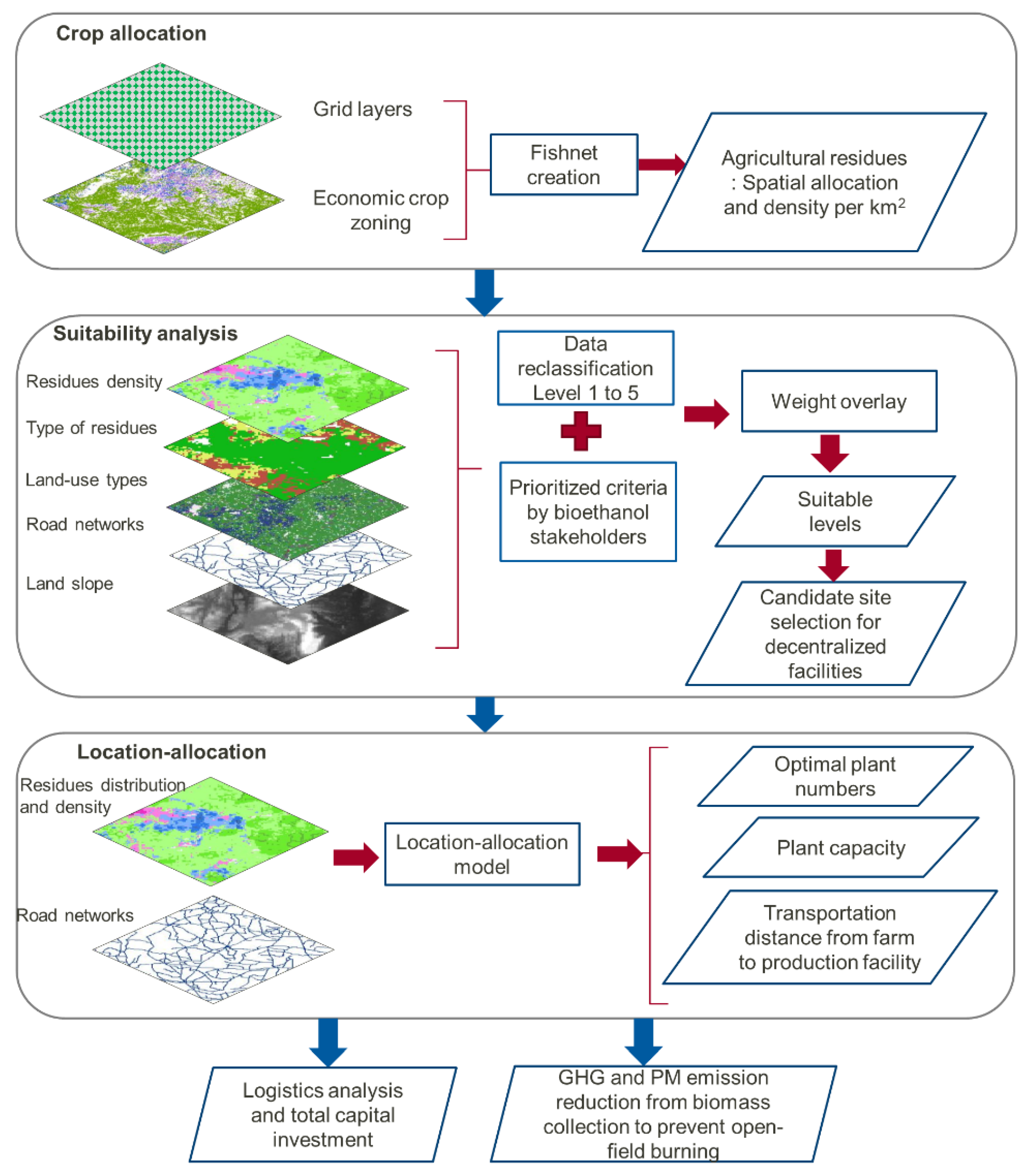
Figure 1 illustrates a flowchart indicating the input dataset, modelling procedures used in this study, and the expectable outputs. Spatial analysis and network analysis are conducted through the ArcGIS 10.8.1
® software by ESRI (Environmental Systems Research Institute, Redlands, CA, USA). Input spatial information used in the modeling analysis was collected both in vector and raster format. For non-spatial inputs, data were collected from statistical reports and related publications, which are elaborated upon in the following sections. However, with respect to the calculation of logistics and investment costs based on the same baseline, the current work did not consider the modification process.
2.1. Regional Case Studiues and Gricultural Residues Allocation
As previously clarified by Jusakulvijit et al., the most generated residues in Thailand could be obtained from crop plantation comprising sugarcane residues (SRs), cassava residues (CRs), rice residues (RRs), and palm residues (PRs), providing availability and density distributed differently in each region of Thailand [
13]. These types of biomass are selected as the targeted feedstocks in this study with a summary of the total production yields in
Table 1. The residue productivity, as obtained from the previous study, refers to the conversion from crop productivities based on the national statistics database according to the Office of Agricultural Economics and residue-to-crop ratio derived from the literature [
13,
49].
In this study, we divided the country level into 4 sub-boundaries on the basis of administrative boundaries and the regional characteristics of biomass availability according to previous schematic findings of crop residues [
13]. The context of existing bioethanol facilities also differentiated the backgrounds of each targeted region. Case studies R1_South and R2_North aim to depict the construction of decentralization due to non-located facilities in this area. Meanwhile, the case of R3_Northeast accommodates the current infrastructures for 8 production units combined with new candidate plants. For the case R4_Central, biomass allocation and logistics analysis were performed by considering only currently operational facilities, with 17 production facilities in this region.
Based on the provincial scale of crop residue availability, residue distribution was created into 1 × 1 km
2 pixels of biomass distribution by incorporating a layer of economic crop zoning, a district scale of residue production, and fishnet layers from the fishnet tool of ESRI ArcGIS 10.8.1, following the procedure by Wochele et al. and Perpiñá et al. [
50,
51]. The economic crop zoning in the shapefile format was acquired from the Land Development Department [
52]. After that, only one type of residue that contributed the maximum production was selected in order to represent the production per one grid cell. The precise scales of resource allocation could be obtained to be further used in the suitability analysis and the location–allocation model.
2.2. Geophical Indicators as Input Multi-Criteria
In the initial process of identifying suitable locations, geographical criteria comprising ‘residue density’, ‘type of residue’, ‘land use type’, ‘proximity to road network’, and ‘slope’ were accommodated in this study. The weights of important input attributes used in the suitability analysis were normalized from the Delphi-AHP process and applied in the input layers [
53]. The scores of criteria prioritizations after the normalization from the publication are summarized in
Table 2.
Table 2.
Criteria for applying suitability analysis.
Table 2.
Criteria for applying suitability analysis.
| Criteria | Input Data Sources and References | Assumption of Preferable Conditions (Suitability Level 5) | References
for Criteria
Assumption | Criteria Weights
as Normalized from the AHP by Jusakulvijit et al. [%] [53] |
|---|
| Residue density | [49] | Preferable residue density depends on regional distribution. Due to uneven distribution, reclassification is created based on Jenks’ natural breaks. | [54] | 23 |
| Types of residue | [13] | Preferential levels are determined from the previous study, classified from the highest values of residues-to-ethanol convertibility to the lowest. Cassava residues > palm residues > sugarcane residues > rice residues | [13] | 19 |
| Land use type | [55] | (paddy fields, field crops, perennial, orchard, horticulture, pasture and farm house, rangeland, industrial land, other built-up land, integrated farm/diversified farms). | [40,56] | 20 |
Road network
from OpenStreetMap (OSM) | [57] | Proximity 0–3 km from roads. | [58] | 18 |
| Slope | Digital elevation model (DEM) published by the United States Geological Survey (USGS) [59] | Slope < 10%.
Higher slope percentage could affect the residue removal rates and also lead to higher construction cost from land leveling process. | [58,60,61] | 20 |
| Total | | | | 100 |
2.3. Suitability Analysis
In the current work, the analysis for determining suitable locations was conducted by using integrated tools combining GIS applications and multi-criteria decision analysis (MCA) [
58]. The integrated methods of GIS-MCA, as a tool for suitability analysis, are broadly used in many studies related to location identification. To incorporate the opinions in decision-making methods, multi-criteria evaluation can account for the opinions from actual players [
28,
62]. Dealing with MCA in this study, the analytic hierarchy process (AHP) was adopted in the combined tools to consider the important levels of regarded parameters [
44,
45].
In order to propose specific locations for decentralized biorefinery development, suitability analysis was applied in this study. Firstly, the values of input spatial layers were reclassified into 5 levels since each parameter has a different range of values. Then, the value of
ith pixel in the
kth level of preference of criteria layers (
) could be derived. Following that, the normalized weights of each parameter (
), as derived from
Section 2.2, were applied to respective meshed polygons to determine the suitability index, as described in Equation (1) through the weighted overlay function in ArcGIS. The output map illustrates the suitability levels which indicate indexed scores representing preferential levels 1 to 5 (
).
Since suitable locations are suggested under the 1 × 1 km2 resolutions, there are several suitable points that share the same district (Amphoe level: the second sub-divided administrative boundary of Thailand). In order to prevent the supply competition between adjacent bioethanol producers, we summarized multiple points to a single point to be used as a candidate production plant per district by dissolving the centroids among suitability level 5, which share the same district boundary through the functionality on ArcGIS.
2.4. Location–Allocation Model
The location–allocation model was applied to allocate input materials to production facilities within the catchment areas. From preselected suitable candidate locations, the location–allocation model enabled the selection of optimal plants (
n) that could connect the shortest distances from the source point
to the candidate facility
(
) via
p-median problem solving [
54]. Equation (2) describes the target of the computation based on the input vector layer of the road network, locations of the candidate facilities, and the residue weights. The impedance cut-off at 80 km was established as a threshold distance restricting the maximum radius from the facility to the resource supply. Equations (3)–(5) refer to the condition that the biomass from each source is limited to assign to only one facility in order to avoid overlapping between demand facilities. Then, biomass resource weights at point
(
) could be supplied to facility
only when the facility is still open in the respective area. Finally, when assigning the numbers of facilities to
, the total numbers of selected candidate facilities are denoted to be equal to
.
In this study, we run the location–allocation model for
V = {1, 2, …,
n}. The set-up numbers (
n) for R1_North, R2_South, R3_Northeast, and R4_Northeast were 25, 25, 45, and 17, respectively. By increasing the set-up numbers of installing units, it was possible to illustrate the coverage rates of residual biomasses. The allocated residues to the proposed facilities could then be used to determine the potential capacity from the supplied feedstocks.
s.t.
where
is an indicator of the assigned residue. If it is equal to 1 when there is agricultural residue assigned to facility j and 0 if not,
indicates the candidate points when it is selected as facility point
or
.
Collectable Residue Quantity and Bioethanol Production Capacity
From the location–allocation model, the quantity of available wet biomass in the catchment area could be obtained (
AWB). However, to pursue the biomass quantity that could reflect realistic values, the usable biomass per biorefinery facility (
was calculated through Equation (8) by dividing it by
n numbers of optimal plants. The
was applied with a usable biomass rate (
) and a collectable residue ratio (
), which were taken as 0.85 and 0.50, respectively [
36,
63]. This collectable ratio was also considered based on the functionality of soil erosion protection from left-over crop residues. Meanwhile, considering the quantities of residues with a bioenergy purpose, farm accessibility rates indicating the farmland factor (
) and the transportation and storage loss (
) were also applied in the calculation [
36]. For the moisture content (
), the dataset for each type of biomass was acquired from the previous reports in the literature [
13]. Then, through Equations (8) and (9), the annual dry biomass production based on the average per facility (
) could be formulated.
Then, the theoretical bioethanol production capacity (
) was estimated based on the usable dry biomass quantity (
) fed per biorefinery and the biomass to bioethanol convertibility (
), as presented in Equation (10). The residue-to-ethanol conversion factors (
) have been retrieved in the previous findings by Jusakulvijit et al. [
13] The value of parameters used in the calculation can be referred in
Supplementary Table S1 with input data sorted from the literature [
36,
63,
64].
2.5. Logistics Analysis and Investment Costs
2.5.1. Logistics Cost Analysis
Logistics cost estimation conducted in this study comprised the costs from biomass handling, collecting, loading, and delivering from resources to biorefineries. On the other hand, we did not include the biomass pre-processing procedures and the in-plant processing cost at the biomass storage process. The costs associated with nutrient replacement from residue utilization in this study are also not included since the calculation already concerns the collection fraction for bioenergy purposes at 50% of the available biomass. The logistics costs were calculated separately through spreadsheet model development under each regional area using spatial analysis, referring to the analysis of Sultana et al. [
65]. Input monetary data for cost calculation in this study were collected from the literature and adjusted with an inflation index to the year 2020. For the price regarding fuel consumption in biomass transportation, values were collected from the diesel selling price in 2020 and converted from THB to USD [
66]. Regarding the parameters for the transportation cost calculation, variable values were collected from the literature, as summarized in
Supplementary Table S1. (detailed input parameters see Refs. [
67,
68,
69,
70,
71,
72,
73]).
In this study, the collecting methods were generalized under the same baling method for every type of biomass since the bale processing costs are lower than the pelletized biomass [
66]. Equation (11) elaborates the formula of the biomass collecting and handling cost (
, constructed from the processing costs of biomass shredding (
), biomass raking (
), biomass baling (
, biomass twining (
), biomass storage (
), farmer premium (
), biomass grinding to size 10 mm (
), and tub-grinding operation (
).
Next, the transportation cost regarding biomass delivery (
) was carried out following Equations (12) and (13). The cost was estimated from the portion of truck delivery and the biomass loading–unloading cost from trucks. The delivery cost was formulated from multiplying
with the tortuosity factor (
[
39], the variable of the truck transport per weight per distance in a trip (
, and the delivery rounds calculated from usable biomass weight divided by the truck capacity (
. For the biomass loading–unloading cost, the loading–unloading factor (
) was applied in the equation.
Finally, the logistics cost per production facility (
and the unitary logistics cost (
per production volume were computed in the study, following Equations (14) and (15). Then, the logistics cost results per delivered feedstock were used for comparing the transportation costs at different scales of bioethanol production capacity in the later section.
where
is an average round trip distance from residue collection delivered to bioethanol refineries and
represents the number of connected routes derived from the location–allocation model.
2.5.2. Total Capital Investment (TCI) Estimation
TCI is one of the most important factors for determining the optimal scale when designing a decentralized scheme for comparing the production size with an estimated logistics cost [
74]. Technically, to address the precise investment cost, it is necessary to break down the cost of associated factory elements. In this study, however, the cost estimation process was considered from the baseline non-linear scale factor (
), as mentioned in the technical report by Humbird et al. [
75]. The exponent factor
= 0.6 was applied in none-linear regression, as described in Equation (16). The new TCI could be computed with an input base plant capacity (
and base cost (
) of 230.58 mL year
−1 and USD 594.28 million, respectively, which are values reported by Humbird et al. [
75]. Thus, the expectable new cost (
) could be obtained depending on the new input plant capacity (
), as estimated in this study.
2.6. Emission Abatement from Open Field Burning
GHG emissions and atmospheric emissions in Thailand mainly occurred from sugarcane and rice cultivation due to the process of post-harvest biomass [
15,
16], whereas in general the post-harvest residues from palm plantation are being left on plantation areas without the incinerating process [
76]. The open-field burning process emits GHGs, as we considered CO
2, CH
4, and N
2O in this study, and health-threatening particulate matters (PMs) such as PM
10 and PM
2.5 [
15,
77].
Firstly, the total emission factor (
) for each type of residue was formulated from the summation of emission factors of CO
2, CH
4, and N
2O, as written in
,
, and
, respectively (in Equation (17)). For
and
, global warming potential (GWP) values of 25 and 298 were multiplied in order to convert the equivalent of kg CO
2 [
78].
Then, in order to calculate the GHG abatement potential and air pollutants, as presented in Equation (18), the
was multiplied with a fraction of biomass subjected to open burn (
), and the combustion factors (
) which correspond to each kind of agricultural residues and the collectable dry residue quantity (
). The methods performed by Sornpoon et al. and Gadde et al. are referenced in the current study [
77,
79]. Meanwhile, the amount of PM reduction potential was estimated from multiplication with emission factors of PM
2.5 (
and PM
10 (
), as shown in Equation (19). The parameter values used in Equations (17)–(19) are summarized in
Supplementary Table S2 compiled from the available data in the literature (see Refs. [
80,
81,
82,
83,
84,
85,
86,
87,
88,
89,
90].
3. Results
3.1. Agricultural Residues Allocation
High resolutions of biomass allocation were successfully illustrated, indicating available yields per pixel (kg km
−2) of SRs, CRs, RRs, and PRs. The distribution of four types of agricultural residue was also classified in a gridded map on ArcGIS into different categorized production densities, as shown in
Supplementary Figure S1. Different colors indicate a variety of biomass types and the maximum density of residue generation per square kilometer.
A summary of the distributed biomass quantifications is categorized in each region in
Table 3. It can be observed that R3_Northeast produced the highest biomass availability rates, whereas the lowest available biomass was found in R1_North. In terms of biomass type categorization, the most generated residues were SRs, followed by RRs. The least generated biomass was PRs, which was mostly collectable in R2_South. In terms of cultivation areas, the largest cultivation farms were found in the R3_Northeast, occupying an area of 139,377 km
2. The dominant residues were from sugarcane’s post-harvest SRs. Following that, the second largest farm areas were found in the R1_North, with SRs representing a majority biomass allocation. A similar size was allocated to the total cultivation areas in R4_Central, i.e., the most available biomass, dominated by RRs. Finally, the R2_South constituted the smallest cultivation area with palm plantation and paddy fields. In total, for Thailand’s potential farms as a whole nation, we identified 296,858 km
2 with collectable biomass in this study.
3.2. Site Selection from Suitability Analysis
An exemplary output map (see
Figure 2) of suitable areas was classified into five levels, as illustrated in
Figure 2b. The most suitable areas at level 5 were illustrated in red raster layers. We could identify the suitable level 5 into one specific candidate location per district boundary by dissolving the points of extensive layers, as presented in
Figure 2c. As a result, R3_Northeast found the greatest numbers of suitable locations, resulting in 221 areas. R3_Northeastern was distributed as the most widespread area because paddy fields were the largest arable land in this region, and had the highest RR production. Following that, R1_North and R2_South had 152 and 121 areas. In sum, 494 candidate areas were proposed in total for simulating the decentralized installation. Suitable areas in R2_South were favorably located in the same spatial patterns as PR availability. For the suitability analysis, results of every region can be inferred in
Supplementary Figures S2 and S3.
3.3. Decentralized Bioethanol Production Design from the Location–Allocation Model
With the location–allocation model, optimal biorefineries in four regions were selected from candidate suitable plants in addition to the existing operational plants. Visualizations of the connected routes from defined biorefineries to the captured residue resources are presented in
Figure 2d, whereas changes in residue coverages from increasing biorefinery numbers in the regional boundaries are shown in
Supplementary Figure S4. It can be noted that bioethanol facilities are likely to be chosen in high-density biomass areas as the first priority as a significant indication can be observed in R1_North. The model succeeded in allocating the feedstock biomass supply without conflicts between refineries.
Figure 3 demonstrated relations of biomass utilization rates and the average potential bioethanol capacities per plant corresponding to the increasing numbers of set-up installation facilities. Although increasing production units led to incremental residue utilization rates, there were peak points which represented the maximum biomass coverage (utilization rates). Thus, raising installation numbers after the maximum coverages also caused declines in biomass collection rates because a certain amount of the overall supply per region has to be shared to more producers. The case of R2_South illustrates the collectability which declined after increasing the number of facilities over the maximum due to condensed installation limited by accessible biomass supply.
As a result, we could identify the greatest collectable amounts in R1_North, R2_South, R3_Northeast, and R4_Central as 13,568, 37,304, 321,085, and 11,010 kTons year−1, respectively. The maximum biomass coverage rates in respective regions were 91.8, 90.8, 90.5, and 79.7%. According to the outcomes of maximum collection, the optimal installation numbers were suggested to be 18, 7, 30, and 16 units in R1_North, R2_South, R3_Northeast, and R4_Central, respectively. Biomass utilization rates also created different results in different cases, both with and without considering current plants. In the case of considering only existing locations, R4_Central has showed that the biomass collectable curve almost reached the plateau after installing to approximately five units. It is possibly due to the condition of fixed locations which controlled the modeling opportunities to expand to broader areas.
3.4. Logistics Analysis and Estimated Capital Investment Cost
Delivery distances were derived from the location–allocation model.
Figure 4 displays the analysis outcomes of the unitary logistics cost per bioethanol productivity associated with installation units. Every regional case study showed a lower logistics cost in line with more numbers of installation. Among four cases, the unitary logistics cost in R2_South was found to be the highest in the range of USD 1.73–2.46 L
−1. Nonetheless, R2_South displayed the largest drop in the logistics cost (almost 30%) by increasing facility numbers. The model succeeded in saving logistics costs due to an improvement in searching resources with higher conversion factors, specifically referring to RRs, in addition to PRs in this case. On the other hand, R1_North, R3_Northeast, and R4_Central could benefit from the CR availability, resulting in lower logistics costs. The R4_Central showed the lowest rate in the range of USD 1.18–1.32 L
−1, which did not change significantly when increasing the number of facilities.
Figure 5 illustrates correlations between the unitary logistics cost per delivered feedstocks and bioethanol production scales in different regional case studies. In every case, it is noticeable that when the production capacity per unit is smaller due to more installed facilities, the logistics cost per unitary feedstock delivery became cheaper. The results demonstrated the benefits of locating more facility units for shortening distances from feedstock resources. The cost curves vary on each region, and are structured from different geographical features and residue availabilities. Rapid increases in unitary logistics costs, from the smallest to the flat curve at different points of the production capacity, were evident. For example, R1_North reached a stable transportation cost per feedstocks after a production capacity of around 50 mL year
−1. The curve changes from logistics analysis can be used as a development framework for optimizing the productivity if the logistics cost is reduced.
3.5. Estimated Capital Investment Costs
In light of the TCI computation based on production capacity,
Figure 6 shows the changing curves of the TCI according to more plant installations. As consistent with every scenario, the TCI was cheaper when there were fewer exhibited production units in the region, which refers to a larger capacity per plant. Therefore, with more numbers of plant installation, the production capacity per unit become smaller, leading to more expensive TCIs. The expectable ranges of the TCI in R1_North were observed to range between USD 3.33 and 6.93 L
−1 as the installation plants increased from 1 to 25 plants. For R2_South, the estimated TCI ranged between USD 1.67 and 4.98 L
−1. Following that, the price range of the TCI in R3_Northeast within 1–25 plants varied from USD 1.17 to 2.48 L
−1, making it the most cost-effective solution due to the large volumes of productivity in this region. Among four regions, R4_Central became the highest TCI curve since it has the lowest bioethanol production potential, ranging from USD 3.51 to 6.50 L
−1.
In accordance with the optimal installation numbers based on the maximum biomass utilization rates, the results presented the placement of diverse production scales in one region. The illustration in
Figure 7a–d presents geographical mapping of bioethanol scales with the estimation of a capital cost per unit in the respective region. Corresponding to the classified scales, the bubble sizes and categorized colors on the right-hand graphs portrayed the potential scales of the bioethanol refinery. In this study, the proposal construction of bioethanol scales was grouped into four different scales, i.e., ‘small’, ‘medium’, ‘large’, and ‘very large’.
Firstly, R1_North with 18 optimal units resulted in TCIs per bioethanol production unit ranging between USD 3.11 and 20.80 L−1. Plant installations were mostly dominated by a small-size capacity. As the northern area of R1_North is constituted with mountain ranges and high elevated lands, the outcomes of decentralized small-scales seemed to be specifically appropriated to enhance resource accessibility. Next, the TCI results in R2_South clarified the costs ranging from USD 1.91 to 7.13 L−1. In this region, the capacity was found under the category of large-scale production. For R3_Northeast, it was possible to identify all four ranges of production scales, showing the TCI ranges at USD 1.19–5.90 L−1. However, most of production plants fell into large and very large size productions. Large-scale bioethanol productions are generally produced from SRs and CRs where the TCIs showed relatively low rates. Lastly, the outcomes of R4_Central indicate a small-scale production, which could effectively represent decentralized facilities. The TCIs in this region altered between USD 4.37 and 18.73 L−1.
In addition to formulating various scales of biorefineries, we projected the potential scenarios under different assumptions of biomass utilization rates (BURs). The reason for this scenario projection is based on assuming that the participation of biorefineries may not reach 100% of the proposal in reality, due to the fact that smaller scales of producers need to pay unitary TCIs at higher rates. If the biomass utilization may be prioritized, the shadowed areas of BUR at around 80% and 50% indicated the production facilities that are encouraged to be established. For instance, the coverage of BUR 85% in R1_North alluded to biorefinery No. 10, 11, 12, 14, 15 and 17, representing a set of small and medium production units, while BUR 50% covered only two units including No. 10 and 17.
3.6. Emissions and Pollutants Abatement from Biomass Collection
By increasing the numbers of bioethanol production facilities, the amount of residue collection is expected to contribute to expectable GHGs and pollutant eliminations. The result of GHG emission abatement curves, as compared to the emission rates without biomass utilization under different numbers of refineries, is presented in
Supplementary Figure S5. The maximum generated values of complete combustion from left-over biomass was found to emit 9.1, 0.5, 167.1, and 9.4 M ton CO
2 eq of GHG emissions in R1_North, R2_South, R3_Northeast, and R4_Central, respectively. Nonetheless, when the biomass residues were collected, significant abatement could be observed.
Table 4 summarized GHG and particulate matter (i.e., PM
10 and PM
2.5) reduction potential from the maximum biomass collection in each location. A comparison among four regions unveiled that R3_Northeast resulted in the highest GHG, with a saving potential of PM
10 and PM
2.5 at 153.7 M tons of CO
2-eq year
−1 reaching 605.3 and 552.8 k Tons year
−1, respectively. An estimation of this region is around 90% of a whole estimated national emission.
4. Discussion
4.1. Spatial Distribution and Biomass Allocation to Decentralized Facilities
The bioethanol potential convertibility from SRs, CRs, RRs, and PRs in the decentralized units was previously evaluated between 0.38 and 1.39 L bioethanol per kg of dry matter, based on the biomass production in 2018 [
13]. As such, this study proved that the conversion of those figures can utilize scattered crop residues to potentially reach 13,444 million L of bioethanol from the maximum collectable residues.
The estimated amount of bioethanol can not only substitute fossil fuels but also reduces additional GHG emissions, when the agricultural residues are no longer burned on the field. We could prove these benefits in terms of the GHG emission reduction by transitioning from centralization to decentralization. Taken as the preliminary estimation, if the generated agricultural residues are completely utilized in bioethanol production, the CO
2 abatement from substituting the fossil-based gasoline can be expected to reach around 21.99 M tons of CO
2 (calculated based on emissions from direct combustion) on top of the abatement from avoiding the open-burning action [
91]. However, in order to scrutinize the precise reduction effect, an overall supply chain of bioethanol production needs to be accounted for the life-cycle GHG emissions [
92,
93].
In this paper, the spatial features of input variables were created based on 1 × 1 km2 in a high resolution. The constructed grid cells from geographic layers successfully enabled the function of suitability analysis and location–allocation modeling. By accommodating GIS-MCA, the characteristics of suitable spots in respective regions can effectively reflect the suitable areas with the high density of agro-residues. For example, R1_North highly recommended areas that were mostly in the lower part of the north, i.e., non-mountainous areas with a high density of biomass availability and cultivation, as well as industry-oriented land use types. Similarly, suitable areas in R2_South are restricted by preserved forests and extended mountain ranges in spite of high densities of palm plantation.
Although accuracy suitability analysis can be improved from applying additional spatial information (e.g., water sources or power utility systems) [
94], the geographic results from suitability analysis in this study are in line with the suitable locations assessed by Cheewaphongphan et al., who addressed the locations of biomass power plants from a rice straw for different utilization technologies [
15]. Based on candidate points, when existing production has not been originally situated, there is more freedom for the model to seek out the most optimal sites and expand catchment areas to collect residues.
4.2. Logistics for Biomass Supply Chain
In this study, the connection between biorefineries and supply sources was assigned based on the actual spatial information of road network in Thailand. This approach effectively and accurately determined the adjacent resources allocated to producers. The approach in the study is distinctive from some of the literature [
44,
95] based on the assumption of limiting radial distances to avoid exceeding 80 km. However, according to the modeling execution, acquired output data ranged between 37 and 55 km. These figures demonstrate that the highest economic viability in biomass-to-biofuel industries is between 45 and 80 km [
40,
51].
With the restriction of catchment distances, it was possible to limit the rising production scales from expanding a longer collecting radius, and also allowed the study to expand biomass spatial coverage from multiplying production units instead of expanding catchment areas. With our simplified logistic analysis approach, we proved that increasing installation units can improve average logistics costs. This significant result could be observed in the case of R2_South, as presented in
Figure 7. Although the case of R2_South resulted in the most expensive logistics cost, the result revealed that R2_South contributed the most significant change following expanding numbers of production refinery per region.
Although trend lines of unitary biomass logistics per delivered feedstock are relatively similar across regions, as presented in
Figure 5, R3_Northeast seemed to gain the most advantageous outcomes owing to the high density of biomass availability and the high potential of the bioethanol conversion ratio. The results also imply that bioethanol convertibility and density per area are influential factors for estimating unitary logistics costs. Thus, the possibility of reducing logistics costs per capacity could be achieved by blending input materials with a high convertible biomass, leading to a higher bioethanol yield.
4.3. Opportunities of Decentralization and Prospect for the Future Development
Decentralized schemes, as proposed in this work, proposed 71 units of decentralized biomass refineries in total. The conceptual designs could be proposed by depicting production units which consolidate different scales (small, medium, and large), as shown in
Figure 7. Since the study did not prioritize the crop type selection, the concept of mixed feedstock could be expected to prevail against the limitations from single-type feedstock, especially regarding the harvesting seasonality. In real practice, SRs are collectable around November to March, whereas CRs can be collected between March and May [
96]. For RRs, the harvesting period is between October and December [
49]. Therefore, the heterogeneous feedstock utilization can potentially compensate production yields between cultivation cycles.
Considering the regions without current invested facilities, R1_North could be used for initiating stand-alone and small-scale production facilities, as R1_North consists of many remote areas with obstacles including high elevation and land slope. Meanwhile, R2_South has more advantages in terms of PRs that can be used with the highest biomass-to-crop ratio. In some areas of R2_South, medium-to-very large scales can be used due to the high generated density of PRs, which require mass production facilities. For R3_Northeast and R4_Central which have operating plants, the existing locations could possibly be used for supplying alternative feedstocks.
In decentralized production scales, the TCI is also a vital factor for determining the project investment scales. Taking R4_Central as an example, TCIs from newly developing plants may cost USD 4.37–18.73 L
−1, which is considered to be around 2–4 times more expensive than some pioneer second-generation plants [
97,
98]. To deal with the economic limitation, integrating the first- and the second-generation technologies could encourage a reduction in capital investment. Another possible solution concerns the adjustment of radii for the catchment area to be larger than 80 km in order to increase the quantity of feedstocks and production scales.
Despite economic challenges, the study demonstrated opportunities of encouraging local producers and farmers to potentially participate in future project developments. To encourage the proposed scheme for policy implications, incentivized mechanisms may become necessary in order to persuade farmers to deliver post-harvested biomass into the bioethanol production chain. One of the important driving factors regards the feedstock selling price that can attract farmers, so they can benefit as value-added incomes along with the main crop production.
5. Sensitivity Analysis
The sensitivity analysis was conducted to observe the effects of variables involving biomass availability, delivery distances, delivery costs, and the fluctuating supplying feedstocks. Firstly, from the study of logistic cost sensitivities, as shown in
Figure 8, the most sensitive parameter in every case study was indicated to the delivery distance. The similar trends across regions demonstrate that the costs increase as the delivery distances become longer, and vice versa. The next influential factor was the delivery cost per kilogram per kilometer. On the other hand, it is noticeable that the influence of varying quantities of biomass supply were hardly affected by the cost changes within ±30% from the base case.
Another clarification is associated with the missing specific type of input feedstocks due to the seasonality or supply allocation. As a result, except for the R2_South, logistics costs in every region are sensitive to unavailable SRs, since SRs offer benefits including the high density of availability. On the contrary, the exclusion of RRs resulted in lower logistics costs, as displayed in
Figure 8a,c. The exclusion of RRs positively affected the logistics costs due to the fact that it offered the lowest bioethanol convertibility. Interestingly, the most significant logistics cost reduction in R2_South was offered from factoring out PRs as input feedstocks owing to the massive quantity of collectable residues which increases the transportation cost. Hence, reducing the input PRs can also be beneficial in the logistics cost reduction.
In addition to the sensitivity of logistics costs,
Figure 9 showed the sensitivity analysis results of the TCI according to changing variables. As a result of changing biomass availability, among four regions, R3_Northeast demonstrated the most sensitive TCI changes, as the price ranges showed the largest span of the lowest and the highest price, i.e., USD 1.89 L
−1 to USD 2.42 L
−1. On the other hand, the least sensitive scenario depending on biomass availability was discovered in R2_South.
The TCI directly relies on the production scales. Hence, the densities of available biomass and bioethanol conversion factors from different types of biomass are important indicators for estimating the production capacity. We demonstrated the absence of each kind of biomass to detect the effects from different types of input feedstocks. Without each type of biomass, the TCI soared, particularly from the scenario without SRs in R1_North, R3_Northeast, and R4_Central. For R2_South, unavailable PRs affected the TCI the most, as it costs more than the double price of the TCI from the base case scenario to over USD 6.00 L−1.
6. Conclusions
The agricultural residues from post-harvesting sugarcane, cassava, rice, and palm were proposed as feedstocks for bioethanol production. In this study, the geographical variables were created at 1 × 1 km2 grid-scale resolutions, providing mapping information of spatial biomass availability. By implementing the integrated GIS-based suitability analysis and prioritizing the techno-economic viability, 494 candidate locations were suggested in the model. The goal to maximize biomass collection rates was achieved through the location–allocation model to determine the feasible numbers of installation units, resulting in 18, 7, 30, and 16 optimal facilities in the north, south, northeast, and center of Thailand, respectively. In total, 71 locations were chosen in this work, revealing the optimal numbers of installation facilities that cover 80–92% of spatially available residual biomass rates. The amount of collected residues could contribute to reductions of 170 M tons of CO2-eq GHGs and 1271 k tons of particulate matters, suggesting potential solutions to abolish open-field burning of crop residues.
By installing more decentralization units, cutting logistic costs represents a decline of 10–30%. Nonetheless, exhibiting more biorefineries causes trade-offs from investment costs along with benefits. The range of possible logistics costs in the scope of the nation within 1–25 plant installations was indicated at USD 1.17–2.46 L−1, whereas the total capital investment was in the range of USD 1.17–6.93 L−1. The results can be used as an economic framework for further analysis to verify the minimum bioethanol selling price in the future work.
The proposal of combining different biorefinery scales in respective regions in this study could be taken as a recommendation for policy planning or commercialization in terms of location selection and for determining favorable scales based on optimal installation units. In order to drive the scheme into national policy, plants with a high production capacity may be taken as an installation priority in order to cover 50–85% of available biomass per region, which could be economically attractive for encouraging bioethanol producers in relation to investment costs.
Even though comprehensive operational cost analysis from production process still needs to be assessed, the outcomes of logistics costs and capital costs per ethanol production units can be used as baselines to capture the minimum bioethanol selling price. Future research requires further scenario-based analysis by optimizing decentralized schemes based on crossing dimensions of techno-economic and environmental aspects, which is expected to sustainably enhance lignocellulosic bioethanol development.
Supplementary Materials
The following supporting information can be downloaded at:
https://www.mdpi.com/article/10.3390/su14169885/s1. Figure S1: Spatial allocation of agricultural residues indicating per 1 km
2 grid cell in (
a) R1_North, (
b) R2_South, (
c) R3_Northeast, and (
d) R4_Central case study. Figure S2: Suitability level indicating in (
a) R1_North, (
b) R2_South, and (
c) R3_Northeast. Figure S3: Identification of candidate plants to be used as newly proposed decentralized bioethanol production identifying in 3 regions in (
a) R1_North, (
b) R2_South, and (
c) R3_Northeast. Figure S4: Chosen biorefineries according to location–allocation models under the different assumption of installation numbers resulting in connections to biomass allocation in the catchment areas. Figure S5: GHG and atmospheric pollutants emission abatement of (
a) R1_North, (
b) R2_South, (
c) R3_Northeast, and (
d) R4_Central case study. Table S1: Adjusted cost input for using the logistics analysis model. Table S2: Emission factors for estimating atmospheric pollutants from open-field burning.
Author Contributions
Conceptualization, P.J. and A.B.; methodology, P.J.; software, P.J.; formal analysis, P.J.; data curation, P.J.; writing—original draft preparation, P.J.; writing—review and editing, A.B. and D.T.; visualization, P.J.; supervision, A.B. and D.T. All authors have read and agreed to the published version of the manuscript.
Funding
This doctoral research project was financed by the Energy Conservation Promotion Fund (ENCON Fund) of the Royal Thai Government, Ministry of Energy (Thailand) No. 0606/3025, 4 July 2018. Open access funding enabled and organized by Projekt DEAL. Further financial support was received from the Helmholtz Association of German Research Centres through the PoF 4 program Changing Earth–Sustaining our Future, Topic 5 Landscapes of the Future.
Institutional Review Board Statement
Not applicable.
Informed Consent Statement
Not applicable.
Data Availability Statement
The data that support the findings of this study are available upon reasonable request from the corresponding author, P.J.
Acknowledgments
The authors sincerely thank the editor and reviewers for their insightful comments.
Conflicts of Interest
The authors declare no conflict of interest.
References
- IEA Renewables. Analysis and Forecasts to 2026—Report Extract Biofuels. 2021. Available online: https://www.iea.org/reports/renewables-021/biofuels?mode=transport®ion=World&publication=2021&flow=Consumption&product=Ethanol (accessed on 23 February 2022).
- Energy Policy and Planning Office, Ministry of Energy Thailand. Alternative Energy Development Plan: AEDP2015. 2015. Available online: http://www.eppo.go.th/index.php/en/policy-and-plan/en-tieb/tieb-aedp (accessed on 23 February 2022).
- Department of Energy Business, Ministry of Energy. Statistic Data. Available online: https://www.doeb.go.th/2017/EN_index.html?ln=en#/article/en_statistic (accessed on 1 March 2022).
- Howeler, H.H. Effect of Cassava Production on Soil Fertility and the Long Term Fertilizer Requirement to Maintain High Yields. In The Cassava Handbook: A Reference Manual Based on the Asian Regional Cassava Training Course, Held in Thailand; Centro Internacional de Agricultura Tropical (CIAT): Bangkok, Thailand, 2012; pp. 411–428. [Google Scholar]
- Prapaspongsa, T.; Gheewala, S.H. Risks of Indirect Land Use Impacts and Greenhouse Gas Consequences: An Assessment of Thailand’s Bioethanol Policy. J. Clean. Prod. 2016, 134, 563–573. [Google Scholar] [CrossRef]
- Li, T.; Chen, C.; Brozena, A.H.; Zhu, J.Y.; Xu, L.; Driemeier, C.; Dai, J.; Rojas, O.J.; Isogai, A.; Wågberg, L.; et al. Developing Fibrillated Cellulose as a Sustainable Technological Material. Nature 2021, 590, 47–56. [Google Scholar] [CrossRef] [PubMed]
- Archer, A.; Self, J.; Guha, G.S.; Engelken, R. Cost and Carbon Savings from Innovative Conversion of Agricultural Residues. Energy Sources B Econ. Plan. Policy 2008, 3, 103–108. [Google Scholar] [CrossRef]
- Hoang, T.D.; Nghiem, N. Recent Developments and Current Status of Commercial Production of Fuel Ethanol. Fermentation 2021, 7, 314. [Google Scholar] [CrossRef]
- Karlen, D.L.; Johnson, J.M.F. Crop Residue Considerations for Sustainable Bioenergy Feedstock Supplies. Bioenergy Res. 2014, 7, 465–467. [Google Scholar] [CrossRef] [Green Version]
- Kudakasseril Kurian, J.; Raveendran Nair, G.; Hussain, A.; Vijaya Raghavan, G.S. Feedstocks, Logistics and Pre-Treatment Processes for Sustainable Lignocellulosic Biorefineries: A Comprehensive Review. Renew. Sustain. Energy Rev. 2013, 25, 205–219. [Google Scholar] [CrossRef]
- Kim, S.; Dale, B.E. Comparing Alternative Cellulosic Biomass Biorefining Systems: Centralized versus Distributed Processing Systems. Biomass Bioenergy 2015, 74, 135–147. [Google Scholar] [CrossRef] [Green Version]
- Jacobson, J.J.; Roni, M.S.; Cafferty, K.G.; Kenney, K.; Searcy, E.; Hansen, J. Feedstock Supply System Design and Analysis “The Feedstock Logistics Design Case for Multiple Conversion Pathways”; Prepared for the U.S. Department of Energy Office of Biomass Program Under DOE Idaho Operations Office Contract DE-AC07-05ID14517; U.S. Department of Energy: Washington, DC, USA, 2014; p. 194.
- Jusakulvijit, P.; Bezama, A.; Thrän, D. The Availability and Assessment of Potential Agricultural Residues for the Regional Development of Second-Generation Bioethanol in Thailand. Waste Biomass Valorization 2021, 12, 6091–6118. [Google Scholar] [CrossRef]
- Heo, S.; Choi, J.W. Potential and Environmental Impacts of Liquid Biofuel from Agricultural Residues in Thailand. Sustainability 2019, 11, 1502. [Google Scholar] [CrossRef] [Green Version]
- Junpen, A.; Pansuk, J.; Kamnoet, O.; Cheewaphongphan, P. Emission of Air Pollutants from Rice Residue Open Burning in Thailand, 2018. Atmosphere 2018, 9, 449. [Google Scholar] [CrossRef] [Green Version]
- Yodkhum, S.; Sampattagul, S.; Gheewala, S.H. Energy and Environmental Impact Analysis of Rice Cultivation and Straw Management in Northern Thailand. Environ. Sci. Pollut. Res. 2018, 25, 17654–17664. [Google Scholar] [CrossRef] [PubMed]
- Gadde, B.; Menke, C.; Wassmann, R. Rice Straw as a Renewable Energy Source in India, Thailand, and the Philippines: Overall Potential and Limitations for Energy Contribution and Greenhouse Gas Mitigation. Biomass Bioenergy 2009, 33, 1532–1546. [Google Scholar] [CrossRef]
- Tunpaiboon, N. Krungsri Ethanol Industry Analysis 2019–2021. Available online: https://www.krungsri.com/bank/getmedia/0c42d6fd-18d7-41c1-9369-96dded234800/IO_Ethanol_190710_EN_EX.aspx (accessed on 5 September 2021).
- UNESCAP. Decentralized Energy System. Low Carbon Green Growth Roadmap Asia Pacific. 2004. Available online: https://www.unescap.org/sites/default/files/14.FS-Decentralized-energy-system.pdf (accessed on 12 January 2022).
- Soha, T.; Papp, L.; Csontos, C.; Munkácsy, B. The Importance of High Crop Residue Demand on Biogas Plant Site Selection, Scaling and Feedstock Allocation—A Regional Scale Concept in a Hungarian Study Area. Renew. Sustain. Energy Rev. 2021, 141, 110822. [Google Scholar] [CrossRef]
- Fleischmann, M.; Krikke, H.R.; Dekker, R.; Flapper, S.D.P. A Characterisation of Logistics Networks for Product Recovery. Omega 2000, 28, 653–666. [Google Scholar] [CrossRef]
- Stoklosa, R.J.; del Pilar Orjuela, A.; da Costa Sousa, L.; Uppugundla, N.; Williams, D.L.; Dale, B.E.; Hodge, D.B.; Balan, V. Techno-Economic Comparison of Centralized versus Decentralized Biorefineries for Two Alkaline Pretreatment Processes. Bioresour. Technol. 2017, 226, 9–17. [Google Scholar] [CrossRef] [Green Version]
- Mizik, T. Economic Aspects and Sustainability of Ethanol Production—A Systematic Literature Review. Energies 2021, 14, 6137. [Google Scholar] [CrossRef]
- Kubota, A.M.; Dal Belo Leite, J.G.; Watanabe, M.; Cavalett, O.; Leal, M.R.L.V.; Cortez, L. The Role of Small-Scale Biofuel Production in Brazil: Lessons for Developing Countries. Agriculture 2017, 7, 61. [Google Scholar] [CrossRef] [Green Version]
- Lynd, L.R.; Liang, X.; Biddy, M.J.; Allee, A.; Cai, H.; Foust, T.; Himmel, M.E.; Laser, M.S.; Wang, M.; Wyman, C.E. Cellulosic Ethanol: Status and Innovation. Curr. Opin. Biotechnol. 2017, 45, 202–211. [Google Scholar] [CrossRef] [Green Version]
- Rosales-Calderon, O.; Arantes, V. A Review on Commercial-Scale High-Value Products That Can Be Produced alongside Cellulosic Ethanol. Biotechnol. Biofuels 2019, 12, 240. [Google Scholar] [CrossRef] [Green Version]
- Antizar-Ladislao, B.; Turrion-Gomez, J.L. Decentralized Energy from Waste Systems. Energies 2010, 3, 194–205. [Google Scholar] [CrossRef] [Green Version]
- Lemire, P.O.; Delcroix, B.; Audy, J.F.; Labelle, F.; Mangin, P.; Barnabé, S. GIS Method to Design and Assess the Transportation Performance of a Decentralized Biorefinery Supply System and Comparison with a Centralized System: Case Study in Southern Quebec, Canada. Biofuels Bioprod. Biorefining 2019, 13, 552–567. [Google Scholar] [CrossRef]
- Bruins, M.E.; Sanders, J.P.M. Small-Scale Processing of Biomass for Biorefinery. Biofuels Bioprod. Biorefining 2012, 6, 135–145. [Google Scholar] [CrossRef]
- Kim, S.; Dale, B.E.; Jin, M.; Thelen, K.D.; Zhang, X.; Meier, P.; Reddy, A.D.; Jones, C.D.; Cesar Izaurralde, R.; Balan, V.; et al. Integration in a Depot-Based Decentralized Biorefinery System: Corn Stover-Based Cellulosic Biofuel. GCB Bioenergy 2019, 11, 871–882. [Google Scholar] [CrossRef] [Green Version]
- Kumar, I.; Bandaru, V.; Yampracha, S.; Sun, L.; Fungtammasan, B. Limiting Rice and Sugarcane Residue Burning in Thailand: Current Status, Challenges and Strategies. J. Environ. Manag. 2020, 276, 111228. [Google Scholar] [CrossRef] [PubMed]
- Phairuang, W.; Hata, M.; Furuuchi, M. Influence of Agricultural Activities, Forest Fires and Agro-Industries on Air Quality in Thailand. J. Environ. Sci. 2017, 52, 85–97. [Google Scholar] [CrossRef]
- Delivand, M.K.; Barz, M.; Gheewala, S.H. Logistics Cost Analysis of Rice Straw for Biomass Power Generation in Thailand. Energy 2011, 36, 1435–1441. [Google Scholar] [CrossRef]
- Junginger, M.; Faaij, A.; Van Den Broek, R.; Koopmans, A.; Hulscher, W. Fuel Supply Strategies for Large-Scale Bio-Energy Projects in Developing Countries. Electricity Generation from Agricultural and Forest Residues in Northeastern Thailand. Biomass Bioenergy 2001, 21, 259–275. [Google Scholar] [CrossRef]
- Mukherjee, I.; Sovacool, B.K. Palm Oil-Based Biofuels and Sustainability in Southeast Asia: A Review of Indonesia, Malaysia, and Thailand. Renew. Sustain. Energy Rev. 2014, 37, 1–12. [Google Scholar] [CrossRef]
- Vijay Ramamurthi, P.; Cristina Fernandes, M.; Sieverts Nielsen, P.; Pedro Nunes, C. Logistics Cost Analysis of Rice Residues for Second Generation Bioenergy Production in Ghana. Bioresour. Technol. 2014, 173, 429–438. [Google Scholar] [CrossRef]
- Aden, A.; Ruth, M.; Ibsen, K.; Jechura, J.; Neeves, K.; Sheehan, J.; Wallace, B.; Montague, L.; Slayton, A.; Lukas, A.J. Lignocellulosic Biomass to Ethanol Process Design and Economics Utilizing Co-Current Dilute Acid Prehydrolysis and Enzymatic Hydrolysis for Corn Stover; National Renewable Energy Lab.: Golden, CO, USA, 2002. [CrossRef] [Green Version]
- Shahrukh, H.; Oyedun, A.O.; Kumar, A.; Ghiasi, B.; Kumar, L.; Sokhansanj, S. Techno-Economic Assessment of Pellets Produced from Steam Pretreated Biomass Feedstock. Biomass Bioenergy 2016, 87, 131–143. [Google Scholar] [CrossRef]
- Miao, Z.; Shastri, Y.; Grift, T.E.; Hansen, A.C.; Ting, K.C. Lignocellulosic Biomass Feedstock Transportation Alternatives, Logistics, Equipment Confi Gurations, and Modeling. Biofuels Bioprod. Biorefining 2012, 6, 246–256. [Google Scholar] [CrossRef]
- Gonzales, D.S.; Searcy, S.W. GIS-Based Allocation of Herbaceous Biomass in Biorefineries and Depots. Biomass Bioenergy 2017, 97, 1–10. [Google Scholar] [CrossRef] [Green Version]
- Van Holsbeeck, S.; Srivastava, S.K. Feasibility of Locating Biomass-to-Bioenergy Conversion Facilities Using Spatial Information Technologies: A Case Study on Forest Biomass in Queensland, Australia. Biomass Bioenergy 2020, 139, 105620. [Google Scholar] [CrossRef]
- Thomas, A.; Bond, A.; Hiscock, K. A GIS Based Assessment of Bioenergy Potential in England within Existing Energy Systems. Biomass Bioenergy 2013, 55, 107–121. [Google Scholar] [CrossRef]
- Höhn, J.; Lehtonen, E.; Rasi, S.; Rintala, J. A Geographical Information System (GIS) Based Methodology for Determination of Potential Biomasses and Sites for Biogas Plants in Southern Finland. Appl. Energy 2014, 113, 1–10. [Google Scholar] [CrossRef]
- Delivand, M.K.; Cammerino, A.R.B.; Garofalo, P.; Monteleone, M. Optimal Locations of Bioenergy Facilities, Biomass Spatial Availability, Logistics Costs and GHG (Greenhouse Gas) Emissions: A Case Study on Electricity Productions in South Italy. J. Clean. Prod. 2015, 99, 129–139. [Google Scholar] [CrossRef]
- Jayarathna, L.; Kent, G.; O’Hara, I.; Hobson, P. A Geographical Information System Based Framework to Identify Optimal Location and Size of Biomass Energy Plants Using Single or Multiple Biomass Types. Appl. Energy 2020, 275, 115398. [Google Scholar] [CrossRef]
- Hossain, T.; Jones, D.; Hartley, D.; Griffel, L.M.; Lin, Y.; Burli, P.; Thompson, D.N.; Langholtz, M.; Davis, M.; Brandt, C. The Nth-Plant Scenario for Blended Feedstock Conversion and Preprocessing Nationwide: Biorefineries and Depots. Appl. Energy 2021, 294, 116946. [Google Scholar] [CrossRef]
- Tun, M.M.; Juchelkova, D.; Win, M.M.; Thu, A.M.; Puchor, T. Biomass Energy: An Overview of Biomass Sources, Energy Potential, and Management in Southeast Asian Countries. Resources 2019, 8, 81. [Google Scholar] [CrossRef] [Green Version]
- Cheewaphongphan, P.; Junpen, A.; Kamnoet, O.; Garivait, S. Study on the Potential of Rice Straws as a Supplementary Fuel in Very Small Power Plants in Thailand. Energies 2018, 11, 270. [Google Scholar] [CrossRef] [Green Version]
- OAE Office of Agricultural Economics. Available online: http://www.oae.go.th/view/1/Home/EN-US (accessed on 22 May 2021).
- Wochele, S.; Priess, J.; Thrän, D.; O’Keeffe, S. Crop allocation model “CRAM”—An approach for dealing with biomass supply from arable land as part of a life cycle inventory. In Proceedings of the 22nd European Biomass Conference and Exhibition, Hamburg, Germany, 23–26 June 2014; Hoffmann, C., Baxter, D., Maniatis, K., Grassi, A., Helm, P., Eds.; ETA-Florence Renewable Energies: Florence, Italy, 2014; pp. 36–40. [Google Scholar]
- Perpiñá, C.; Alfonso, D.; Pérez-Navarro, A.; Peñalvo, E.; Vargas, C.; Cárdenas, R. Methodology Based on Geographic Information Systems for Biomass Logistics and Transport Optimisation. Renew. Energy 2009, 34, 555–565. [Google Scholar] [CrossRef]
- Land Development Department, Ministry of Agriculture and Cooperatives. Land Economic and Land use Planning. Available online: http://www1.ldd.go.th/ldd_en/en-US/land-economic/ (accessed on 20 June 2021).
- Jusakulvijit, P.; Bezama, A.; Thrän, D. Criteria Prioritization for the Sustainable Development of Second-Generation Bioethanol in Thailand Using the Delphi-AHP Technique. Energy. Sustain. Soc. 2021, 11, 37. [Google Scholar] [CrossRef]
- ESRI, ArcGIS Pro—Data Classification Methods. Available online: https://pro.arcgis.com/en/pro-app/2.8/help/mapping/layer-properties/data-classification-methods.htm (accessed on 8 July 2021).
- Land Development Department, Ministry of Agriculture and Cooperatives. Soil Map and Land Use Map. Available online: http://dinonline.ldd.go.th/ (accessed on 20 June 2021).
- Sharma, B.P.; Edward Yu, T.; English, B.C.; Boyer, C.N.; Larson, J.A. Stochastic Optimization of Cellulosic Biofuel Supply Chain Incorporating Feedstock Yield Uncertainty. Energy Procedia 2019, 158, 1009–1014. [Google Scholar] [CrossRef]
- WFPGeoNode—Thailand Road Network (Main Roads)—WFP GeoNode. 2017. Available online: https://geonode.wfp.org/layers/geonode:tha_trs_roads_osm (accessed on 7 June 2021).
- Sahoo, K.; Hawkins, G.L.; Yao, X.A.; Samples, K.; Mani, S. GIS-Based Biomass Assessment and Supply Logistics System for a Sustainable Biorefinery: A Case Study with Cotton Stalks in the Southeastern US. Appl. Energy 2016, 182, 260–273. [Google Scholar] [CrossRef] [Green Version]
- USGS. Earth Explorer. Available online: https://earthexplorer.usgs.gov/ (accessed on 13 May 2021).
- Taddese, H. Suitability Analysis for Jatropha curcas Production in Ethiopia—A Spatial Modeling Approach. Environ. Syst. Res. 2014, 3, 25. [Google Scholar] [CrossRef] [Green Version]
- Silva, S.; Alçada-Almeida, L.; Dias, L.C. Biogas Plants Site Selection Integrating Multicriteria Decision Aid Methods and GIS Techniques: A Case Study in a Portuguese Region. Biomass Bioenergy 2014, 71, 58–68. [Google Scholar] [CrossRef]
- Famoso, F.; Prestipino, M.; Brusca, S.; Galvagno, A. Designing Sustainable Bioenergy from Residual Biomass: Site Allocation Criteria and Energy/Exergy Performance Indicators. Appl. Energy 2020, 274, 115315. [Google Scholar] [CrossRef]
- Sharma, B.; Clark, R.; Hilliard, M.R.; Webb, E.G. Simulation Modeling for Reliable Biomass Supply Chain Design Under Operational Disruptions. Front. Energy Res. 2018, 6, 100. [Google Scholar] [CrossRef]
- Suh, K.; Suh, S.; Walseth, B.; Bae, J.; Barker, R. Optimal corn stover logistics for biofuel production: A case in Minnesota. Am. Soc. Agric. Biol. Eng. 2011, 54, 229–238. [Google Scholar]
- Sultana, A.; Kumar, A. Optimal Configuration and Combination of Multiple Lignocellulosic Biomass Feedstocks Delivery to a Biorefinery. Bioresour. Technol. 2011, 102, 9947–9956. [Google Scholar] [CrossRef]
- PTT Oil and Retail Business Public Company Limited|Oil Price. Available online: https://www.pttor.com/en/oil_price (accessed on 20 June 2021).
- Napasawat, T. A Study of Fuel Consumption of Trucks. Available online: http://eng.sut.ac.th/ce/ce_course/download/project/7-1-55/20THOSSAPOL%20NAPARSWAD.pdf (accessed on 21 July 2021).
- Agro-Industrial Technology Management (AITM) Kasetsart University, Operations & Value Chain. Available online: http://aitm.agro.ku.ac.th/press/2018/05/09/sugar_cane_transport/ (accessed on 24 June 2021).
- Department of Highways, Regulations of Truck Weight Limits. Available online: http://www.doh.go.th/doh/images/pdf/jkm60-11.pdf (accessed on 18 July 2021). (In Thai)
- Hino Global. Available online: https://www.hino-global.com/products/trucks/hino500/ (accessed on 29 July 2021).
- Delgado, O.; Miller, J.; Sharpe, B.; Muncrief, R. Estimating the Fuel Efficiency Technology Potential of Heavy-Duty Trucks in Major Markets Around the World; Global Fuel Economy Initiative: London, UK, 2016. [Google Scholar]
- Sultana, A.; Kumar, A.; Harfield, D. Development of Agri-Pellet Production Cost and Optimum Size. Bioresour. Technol. 2010, 101, 5609–5621. [Google Scholar] [CrossRef]
- Morey, R.V.; Kaliyan, N.; Tiffany, D.G.; Schmidt, D.R. A Corn Stover Supply Logistics System. Appl. Eng. Agric. 2010, 26, 455–461. [Google Scholar] [CrossRef]
- Kocoloski, M.; Michael Griffin, W.; Scott Matthews, H. Impacts of Facility Size and Location Decisions on Ethanol Production Cost. Energy Policy 2011, 39, 47–56. [Google Scholar] [CrossRef]
- Humbird, D.; Davis, R.; Tao, L.; Kinchin, C.; Hsu, D.; Aden, A.; Schoen, P.; Lukas, J.; Olthof, B.; Worley, M.; et al. Process Design and Economics for Biochemical Conversion of Lignocellulosic Biomass to Ethanol—Dilute-Acid Pretreatment and Enzymatic Hydrolysis of Corn Stover; National Renewable Energy Lab. (NREL): Golden, CO, USA, 2011.
- Singh, R.P.; Embrandiri, A.; Ibrahim, M.H.; Esa, N. Management of Biomass Residues Generated from Palm Oil Mill: Vermicomposting a Sustainable Option. Resour. Conserv. Recycl. 2011, 55, 423–434. [Google Scholar] [CrossRef]
- Sornpoon, W.; Bonnet, S.; Kasemsap, P.; Prasertsak, P.; Garivait, S. Estimation of Emissions from Sugarcane Field Burning in Thailand Using Bottom-up Country-Specific Activity Data. Atmosphere 2014, 5, 669–685. [Google Scholar] [CrossRef] [Green Version]
- IPCC. Summary for Policymakers. In Climate Change 2007: Mitigation. Contribution of Working Group III to the Fourth Assessment Report of the Intergovernmental Panel on Climate Change; Metz, B., Davidson, O.R., Bosch, P.R., Dave, R., Meyer, L.A., Eds.; Cambridge University Press: Cambridge, UK; New York, NY, USA, 2007. [Google Scholar]
- Gadde, B.; Bonnet, S.; Menke, C.; Garivait, S. Air Pollutant Emissions from Rice Straw Open Field Burning in India, Thailand and the Philippines. Environ. Pollut. 2009, 157, 1554–1558. [Google Scholar] [CrossRef] [PubMed]
- IPCC. 2006 IPCC Guidelines for National Greenhouse Gas Inventories—A Primer, Prepared by the National Greenhouse Gas Inventories Programme; Eggleston, H.S., Miwa, K., Srivastava, N., Tanabe, K., Eds.; IGES: Kanagawa, Japan, 2008. [Google Scholar]
- Zhang, J.; Smith, K.R.; Ma, Y.; Ye, S.; Jiang, F.; Qi, W.; Liu, P.; Khalil, M.A.K.; Rasmussen, R.A.; Thorneloe, S.A. Greenhouse Gases and Other Airborne Pollutants from Household Stoves in China: A Database for Emission Factors. Atmos. Environ. 2000, 34, 4537–4549. [Google Scholar] [CrossRef] [Green Version]
- Dennis, A.; Fraser, M.; Anderson, S.; Allen, D. Air Pollutant Emissions Associated with Forest, Grassland, and Agricultural Burning in Texas. Atmos. Environ. 2002, 36, 3779–3792. [Google Scholar] [CrossRef]
- Zhang, Y.; Shao, M.; Lin, Y.; Luan, S.; Mao, N.; Chen, W.; Wang, M. Emission Inventory of Carbonaceous Pollutants from Biomass Burning in the Pearl River Delta Region, China. Atmos. Environ. 2013, 76, 189–199. [Google Scholar] [CrossRef]
- Andreae, M.O.; Merlet, P. Emission of Trace Gases and Aerosols from Biomass Burning. Glob. Biogeochem. Cycles 2001, 15, 955–966. [Google Scholar] [CrossRef] [Green Version]
- Kim Oanh, N.T.; Ly, B.T.; Tipayarom, D.; Manandhar, B.R.; Prapat, P.; Simpson, C.D.; Sally Liu, L.J. Characterization of Particulate Matter Emission from Open Burning of Rice Straw. Atmos. Environ. 2011, 45, 493–502. [Google Scholar] [CrossRef] [Green Version]
- Ni, H.; Han, Y.; Cao, J.; Chen, L.W.A.; Tian, J.; Wang, X.; Chow, J.C.; Watson, J.G.; Wang, Q.; Wang, P.; et al. Emission Characteristics of Carbonaceous Particles and Trace Gases from Open Burning of Crop Residues in China. Atmos. Environ. 2015, 123, 399–406. [Google Scholar] [CrossRef]
- Akagi, S.K.; Yokelson, R.J.; Wiedinmyer, C.; Alvarado, M.J.; Reid, J.S.; Karl, T.; Crounse, J.D.; Wennberg, P.O. Emission Factors for Open and Domestic Biomass Burning for Use in Atmospheric Models. Atmos. Chem. Phys. 2011, 11, 4039–4072. [Google Scholar] [CrossRef] [Green Version]
- Jenkins, B.M.; Bhatnagar, A.P. On the Electric Power Potential from Paddy Straw in the Punjab and the Optimal Size of the Power Generation Station. Bioresour. Technol. 1991, 37, 35–41. [Google Scholar] [CrossRef]
- Christian, T.J.; Kleiss, B.; Yokelson, R.J.; Holzinger, R.; Crutzen, P.J.; Hao, W.M.; Saharjo, B.H.; Ward, D.E. Comprehensive Laboratory Measurements of Biomass-Burning Emissions: 1. Emissions from Indonesian, African, and Other Fuels. J. Geophys. Res. Atmos. 2003, 108, D23. [Google Scholar] [CrossRef]
- Hays, M.D.; Fine, P.M.; Geron, C.D.; Kleeman, M.J.; Gullett, B.K. Open Burning of Agricultural Biomass: Physical and Chemical Properties of Particle-Phase Emissions. Atmos. Environ. 2005, 39, 6747–6764. [Google Scholar] [CrossRef]
- U.S. Department of Energy, Alternative Fuels Data Center. Fuel Properties Comparison. Available online: https://afdc.energy.gov/fuels/properties (accessed on 20 June 2021).
- Wietschel, L.; Messmann, L.; Thorenz, A.; Tuma, A. Environmental Benefits of Large-Scale Second-Generation Bioethanol Production in the EU: An Integrated Supply Chain Network Optimization and Life Cycle Assessment Approach. J. Ind. Ecol. 2021, 25, 677–692. [Google Scholar] [CrossRef]
- Daylan, B.; Ciliz, N. Life Cycle Assessment and Environmental Life Cycle Costing Analysis of Lignocellulosic Bioethanol as an Alternative Transportation Fuel. Renew. Energy 2016, 89, 578–587. [Google Scholar] [CrossRef]
- Sultana, A.; Kumar, A. Optimal Siting and Size of Bioenergy Facilities Using Geographic Information System. Appl. Energy 2012, 94, 192–201. [Google Scholar] [CrossRef]
- Teixeira, T.R.; Soares Ribeiro, C.A.A.; Rosa dos Santos, A.; Marcatti, G.E.; Lorenzon, A.S.; de Castro, N.L.M.; Domingues, G.F.; Leite, H.G.; da Costa de Menezes, S.J.M.; Santos Mota, P.H.; et al. Forest Biomass Power Plant Installation Scenarios. Biomass Bioenergy 2018, 108, 35–47. [Google Scholar] [CrossRef]
- Lacombe, G.; Polthanee, A.; Trébuil, G. Long-Term Change in Rainfall Distribution in Northeast Thailand: Will Cropping Systems Be Able to Adapt? Long-Term Change in Rainfall Distribution in Northeast Thailand: Will Cropping Systems Be Able to Adapt? Cah. Agric. 2017, 26, 25001. [Google Scholar] [CrossRef] [Green Version]
- Aui, A.; Wang, Y.; Mba-Wright, M. Evaluating the Economic Feasibility of Cellulosic Ethanol: A Meta-Analysis of Techno-Economic Analysis Studies. Renew. Sustain. Energy Rev. 2021, 145, 111098. [Google Scholar] [CrossRef]
- Losordo, Z.; McBride, J.; Van Rooyen, J.; Wenger, K.; Willies, D.; Froehlich, A.; Macedo, I.; Lynd, L. Cost Competitive Second-Generation Ethanol Production from Hemicellulose in a Brazilian Sugarcane Biorefinery. Biofuels Bioprod. Biorefining 2016, 10, 589–602. [Google Scholar] [CrossRef]
Figure 1.
Flowchart of geographical modelling and analyses in this study.
Figure 1.
Flowchart of geographical modelling and analyses in this study.
Figure 2.
Exemplary mapping results of geographical modelling from GIS-based analyses, beginning with (a) pixeled distribution of agricultural residues, (b) raster layer of suitability levels, (c) areas of suitability level 5 with dissolved candidate points per district, and (d) results of connected lines between refineries and resources.
Figure 3.
Bioethanol production capacity per plant from changes in facility installation and correlation between the biomass removal rate from collection in the catchment area from different plant installation of different regions: (a) R1_North, (b) R2_South, (c) R3_Northeast, and (d) R4_Central. The circle on the plotted graphs referred to a point where the highest biomass utilization rates can be obtained.
Figure 4.
Logistics cost per production capacity correlating with the increasing number of plant installations.
Figure 4.
Logistics cost per production capacity correlating with the increasing number of plant installations.
Figure 5.
Logistics cost per delivered feedstocks at different average production capacities from four regions: (a) R1_North, (b) R2_South, (c) R3_Northeast, and (d) R4_Central. The numbers (Ns) in brackets represent the number of installed units in each region.
Figure 5.
Logistics cost per delivered feedstocks at different average production capacities from four regions: (a) R1_North, (b) R2_South, (c) R3_Northeast, and (d) R4_Central. The numbers (Ns) in brackets represent the number of installed units in each region.
Figure 6.
Total capital investment (TCI) changing by increasing numbers of plant installations.
Figure 6.
Total capital investment (TCI) changing by increasing numbers of plant installations.
Figure 7.
Schematic images of decentralized plants with estimations of total capital investments corresponding to respective production scales in four case studies: (a) R1_North, (b) R2_South, (c) R3_Northeast, and (d) R4_Central. The bubble size represents the production scales, whereas the biomass utilization rates (BURs) are indicated in blue backgrounds.
Figure 8.
Sensitivity of logistics costs corresponding to varying variables under four studied regions: (a) R1_North, (b) R2_South, (c) R3_Northeast, and (d) R4_Central.
Figure 8.
Sensitivity of logistics costs corresponding to varying variables under four studied regions: (a) R1_North, (b) R2_South, (c) R3_Northeast, and (d) R4_Central.
Figure 9.
Sensitivity of TCIs corresponding to varying variables under four studied regions: (a) R1_North, (b) R2_South, (c) R3_Northeast, (d) R4_Central.
Figure 9.
Sensitivity of TCIs corresponding to varying variables under four studied regions: (a) R1_North, (b) R2_South, (c) R3_Northeast, (d) R4_Central.
Table 1.
Characteristics of residual biomass from agricultural sector in Thailand and the potential bioethanol conversion (adapted with permission from Jusakulvijit et al. [
13]).
Table 1.
Characteristics of residual biomass from agricultural sector in Thailand and the potential bioethanol conversion (adapted with permission from Jusakulvijit et al. [
13]).
| Regions | Residue Type (from Large to Small Order) | Total Yields
[Million
Tons] | Estimated Bioethanol
Production
[ML] | Number of Operating Bioethanol Production Facility | Total Production Capacity of Existing Plants
[ML Year−1] | Case Study Name |
|---|
| North | RR–SR–CR–PR | 4.4 | 595.5 | - | - | R1_North |
| South | PR–RR | 72.4 | 8022.2 | - | - | R2_South |
| Northeast | SR–CR–RR–PR | 62.5 | 9099.7 | 8 | 814 | R3_Northeast |
| Central | SR–RR–CR–PR | 34.8 | 2495.6 | 17 | 1337 | R4_Central |
Table 3.
Total residue availability and proportions in different regions [%].
Table 3.
Total residue availability and proportions in different regions [%].
| Regions | Allocated Residues by Regions in Quantity per Year
[k Tons Year−1] and Proportion in Each Region (%) | Total
[k Tons Year−1] |
|---|
| SR | CR | RR | PR |
|---|
| R1_North | 9652 | 2077 | 3034 | 18 | 14,781 |
| (65.3) | (14.1) | (20.5) | (0.1) | (100) |
| R2_South | - | - | 5535 | 35,552 | 41,087 |
| (0.0) | (0.0) | (13.5) | (86.5) | (100) |
| R3_Northeast | 131,647 | 79,138 | 144,104 | 62 | 354,952 |
| (37.1) | (22.3) | (40.6) | (0.02) | (100) |
| R4_Central | 10,437 | 985 | 2221 | 172 | 13,814 |
| (75.6) | (7.1) | (16.1) | (1.2) | (100) |
| Sum at national scale | 151,736 | 82,201 | 154,894 | 35,804 | 424,635 |
Table 4.
Reduction potential of particulate matters (PM10 and PM2.5) when maximum biomass are collected with comparison of four regions.
Table 4.
Reduction potential of particulate matters (PM10 and PM2.5) when maximum biomass are collected with comparison of four regions.
| Region | GHG
[M tons CO2-eq Year−1] | PM10
[k Tons Year−1] | PM2.5
[k Tons Year−1] |
|---|
| R1_North | 8.4 | 29.9 | 25.3 |
| R2_South | 0.4 | 3.0 | 3.2 |
| R3_Northeast | 153.7 | 605.3 | 552.8 |
| R4_Central | 7.7 | 27.7 | 23.4 |
| Total | 170.2 | 665.9 | 604.8 |
| Publisher’s Note: MDPI stays neutral with regard to jurisdictional claims in published maps and institutional affiliations. |
© 2022 by the authors. Licensee MDPI, Basel, Switzerland. This article is an open access article distributed under the terms and conditions of the Creative Commons Attribution (CC BY) license (https://creativecommons.org/licenses/by/4.0/).


