A New Nonlinear Controller for the Maximum Power Point Tracking of Photovoltaic Systems in Micro Grid Applications Based on Modified Anti-Disturbance Compensation

Abstract

In the photovoltaic system, the performance, efficiency, and generated power of the PV system are affected by changes in the environment, disturbances, and parameter variations, and this leads to a deviation from the operating maximum power point (MPP) of the PV system. Therefore, the main aim of this paper is to ensure the PV system operates at the maximum power point under the influence of exogenous disturbances and uncertainties, i.e., no matter how the irradiation, temperature, and load of the PV system change, by proposing a maximum power point tracking for the photovoltaic system (PV) based on the active disturbance rejection control (ADRC) paradigm. The proposed method provides better performance with excellent tracking for the MPP by controlling the duty cycle of the DC–DC buck converter. Moreover, comparison simulations have been performed between the proposed method and the linear ADRC (LADRC), conventional ADRC, and the improved ADRC (IADRC) to investigate the effectiveness of the proposed method. Finally, the simulation results validated the accuracy of the proposed method in tracking the desired value and disturbance/uncertainty attenuation with excellent response and minimum output performance index (OPI).

1. Introduction

Solar power is an essential source of renewable energy, and its technologies are broadly characterized as either passive solar or active solar depending on how they capture and distribute solar energy or convert it into solar power. However, the PV cell has a low out power conversion efficiency, i.e., lower electrical energy since the V-I and V-P characteristics are nonlinear and depend on environmental factors such as solar irradiation and temperature. This makes the PV cell operating point change as the irradiation or temperature and even the load change and it will not operate at the maximum power point (MPP). Therefore, a controlling technique has been proposed in the last decade under the name of maximum power point tracking (MPPT) [1,2,3,4,5,6,7,8,9]. Recently, several control techniques have been proposed as MPPT to extract and track the MPP such as the perturb and observe method (P&O) [10,11,12]; the incremental conductance method (IC) [10,13,14]; the constant voltage and constant current technique, which are known as the classical MPPT control technique [10]; and MPPT based on the control theory such as fuzzy control [15], neural network [16], optimal control [17], and robust control [18]. In [19], the authors introduced a PID controller to dampen the oscillations of the PV voltage and limit it at the nominal value of the battery charging system, while in [20], a fractional order-based MPPT (FOPID-MPPT) for the PV system was proposed, where the controller parameters are tuned using the FOTF toolbox. It was shown that the proposed FOPID controller has a better performance with the improved transient response and better regulation for the output voltage than the PID one. Moreover, two control strategies, namely, the fractional-order PID-based MPPT (FOPID-MPPT) and fractional order terminal sliding mode controller-based MPPT (FOTSMC-MPPT), have been designed in [7]. The results show that both controllers are robust to the system’s uncertainty with a faster response; however, the FOTSMC provided a small control action as compared to the FOPID one [7]. Recently, various research has been proposed to get rid of the effect of the disturbance and uncertainties in the PV system, such as [21], where authors proposed a novel nonlinear PID (NLPID)-based MPPT with integral gain that varies with the instantaneous error. The parameters of the NLPID are tuned using a teaching–learning optimization algorithm (TLBO). Moreover, comparison simulations have been achieved between the NLPID, the conventional PID, IC-MPPT, and P&O-MPPT under varying irradiation and temperature and the results show the effectiveness of the proposed controller in tracking the MPP and robustness against sudden variations as compared to other methods. In [22], the author presents a modified version of the conventional MPPT algorithm, the incremental conductance algorithm (IC), to achieve an efficient tracking of MPP. Moreover, a genetic algorithm (GA) tuned-based PID is also utilized to improve the system and predict the variable step of the proposed method. The simulation results showed the effectiveness of the proposed method in providing fast-tracking, overshoot, and ripple reduction under the changing of the irradiation and temperature as compared to P&O-based MPPT. Meanwhile, in [23], the authors introduced an intelligent discrete nonlinear PID (N-DPID) base MPPT for a PV system with a WFDC motor. The proposed controller keeps the structure of the conventional PID with integral and derivative parts discretized using the forward Euler approach. Moreover, the N-DPID and PID parameters are tuned using two optimization techniques, namely, particle swarm optimization (PSO) and GA. A comparison between N-DPID, PID, and the conventional MPPT algorithm (i.e., P&O and IC) was accomplished and showed that the PSO-tuned N-DPID provides fast MPP tracking, smooth response, and achieves the rated speed of the WFDC motor under rapid changes in irradiation. Finally, the disturbance observer is used to make the system robust against the disturbance and parameter variations [24,25].

Although all the aforementioned studies proposed robust controlling methods to track the MPP whether there is a change in one of the environmental factors or not, a more accurate and effective control technique is proposed in this paper to stabilize the PV nonlinear system, tracking the MPP with a fast and smooth response, moreover providing robustness against disturbances/uncertainties with higher immunity. This control technique is called Active Disturbance Rejection Control (ADRC). It consists of a traditional tracking differentiator, a traditional nonlinear state error feedback, and a traditional extended state observer [26,27,28,29,30,31]. Furthermore, another important part of the PV system configuration is the DC–DC converter. There are different types of this converter, such as boost converter, buck converter, boost-buck converter, etc. [32,33,34].

Motivated by the aforementioned studies, a modified ADRC has been proposed to fulfill the main aim of this work. The main contributions of this paper can be summarized as follows:

i.

A new nonlinear controller is proposed as a new nonlinear state error feedback (NLSEF). The new nonlinear controller consists of a proposed tracking differentiator (TD) combined with a new super twisting sliding mode controller (STC-SM).

ii.

A new nonlinear extended state observer (NLESO) is proposed to estimate the total disturbance of the PV system.

iii.

Last but not least, the modified ADRC is composed of the aforementioned proposed nonlinear controller (i.e., STC-SM) and the proposed NLESO to stabilize the system and track the MPP in the presence of disturbance and parameter variations.

It is important to note that the overall system is designed and simulated using the MATLAB/SIMULINK environment. Furthermore, the parameters of the modified ADRC are tuned using GA as a tuning technique. Furthermore, a multi-objective output performance index (OPI) is used in conjunction with the GA to ensure the effectiveness of the proposed method with minimum control energy and tracking error.

The remainder of this paper is organized as follows: Section 2 introduces the characteristics and modeling of the PV system. Section 3 presents the design and modeling of the DC–DC buck converter. Moreover, the design of the proposed ADRC is presented in Section 4. In addition, Section 4 illustrates the design and convergence of NLESO and the closed-loop stability analysis. Last but not least, the simulation result and the discussion are introduced in Section 5. Finally, the conclusion of this work is presented in Section 6.

2. PV System Characteristics and Modeling

2.1. PV System Modeling

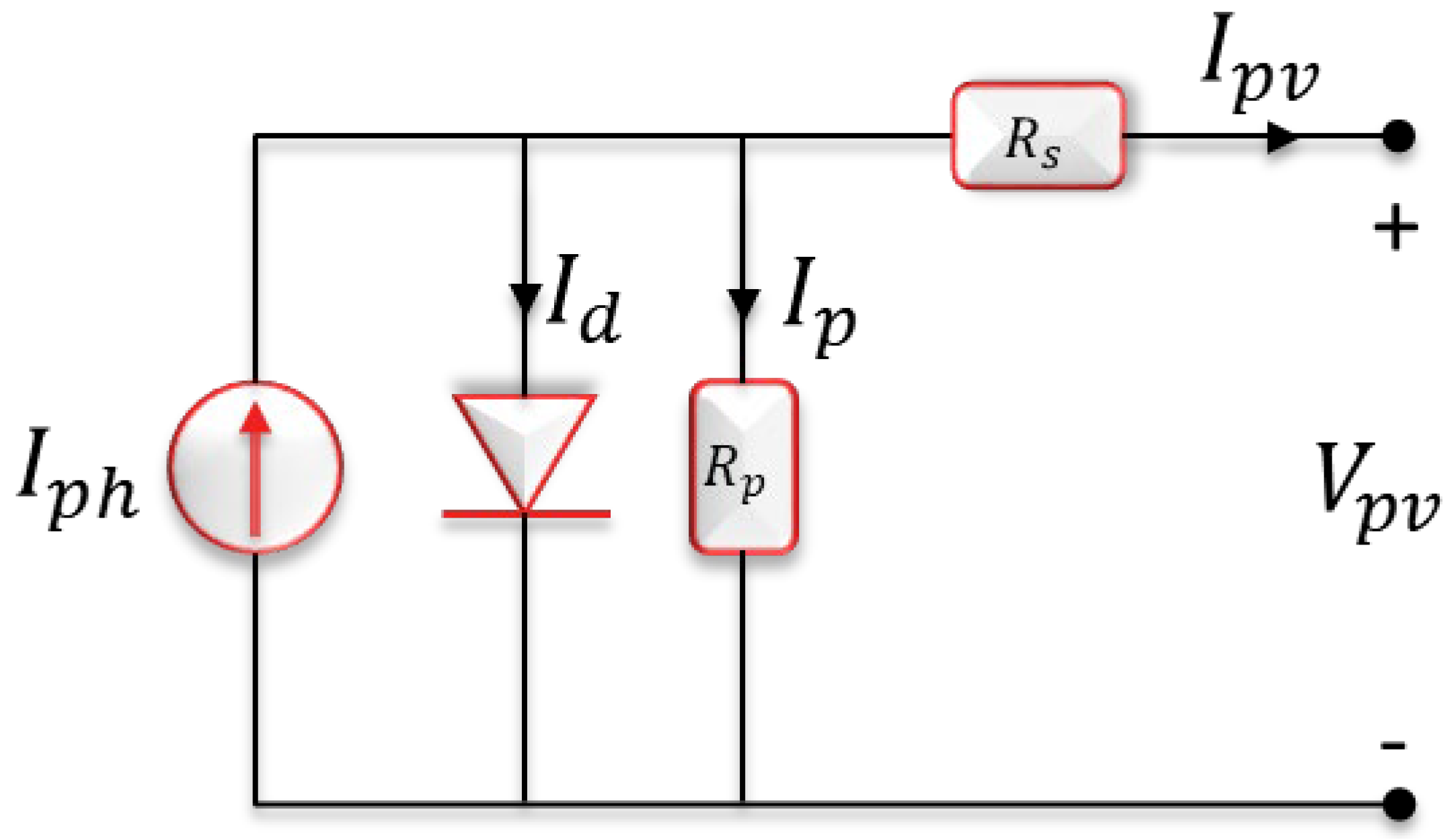
Ideally, the PV cell is represented as a single-diode model. The single-diode model of a solar cell consists of a current source, diode, and two resistances, as shown in Figure 1. In Figure 1, the PV cell is acting as a current source when the light falls on it. Moreover, series resistance and shunt (parallel) resistance are added to simulate the real behavior of PV cells [12].

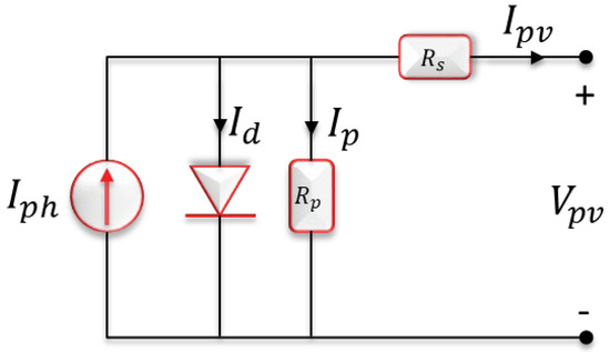
Figure 1. The single−diode PV cell equivalent circuit.

The mathematical modeling of the PV cell is expressed as follows. Firstly, the photocurrent can be expressed as [35]:

$$I_{ph}=\left(I_{S{C}_{STC}}+K_i \left(T-T_{ref}\right)\right)\frac{G}{G_{ref}}$$

(1)

While the diode reverse saturation current can be expressed as follows:

$$I_0=I_{0_{STC}}{\left(\frac{T}{T_{ref}}\right)}^{3}exp\left(\frac{q{E}_{g0} }{\mathbb{A} K_0}\left(\frac{1}{T}-\frac{1}{T_{ref}}\right)\right)$$

(2)

where $I_{0_{STC}}$ is the diode reverse saturation current at STC, which can be expressed as:

$$I_{0_{STC}}=\frac{I_{S{C}_{STC}}}{exp\left(\frac{q{V}_{O{C}_{STC}}}{\mathbb{A} K_0 T_{ref}}\right)-1}$$

(3)

The shunt (parallel) current is expressed as:

$$I_p=\frac{V_{pv}+I_{pv}{R}_s}{R_p}$$

(4)

$$I_d=I_0\left(exp\left(\frac{q\left(V_{pv}+I_{pv}{R}_s\right)}{\mathbb{A} K_0 T_{ref}}\right)-1\right)$$

(5)

Therefore, the PV cell output current is expressed as:

$$I_{pv}=I_{ph}-I_d-I_p$$

(6)

where $\mathbb{A},K_0, q,K_i$, and $E_{g0}$ are the diode ideality, Boltzmann constant, electron charge, current temperature coefficient, and band-gap energy, respectively. $R_s, R_p, T_{ref}, T, G_{ref}$ $G$, and $V_{pv}$ are series resistance, parallel resistance, the temperature at STC (25 °C), cell temperature, irradiation at STC ($1000\frac{\mathrm{w}}{{\mathrm{m}}^2})$, cell irradiance, and PV cell output voltage, respectively.

2.2. PV System Characteristics

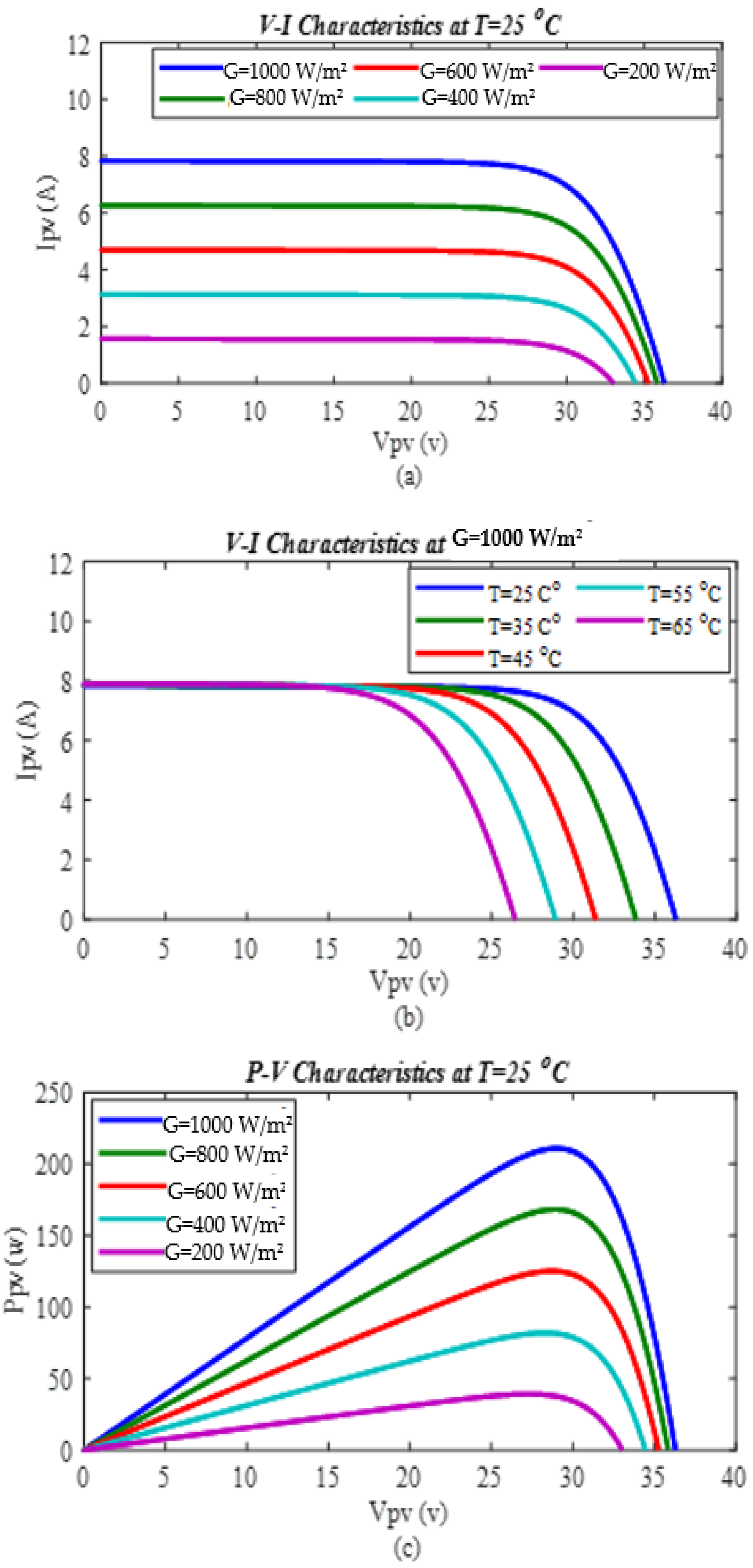
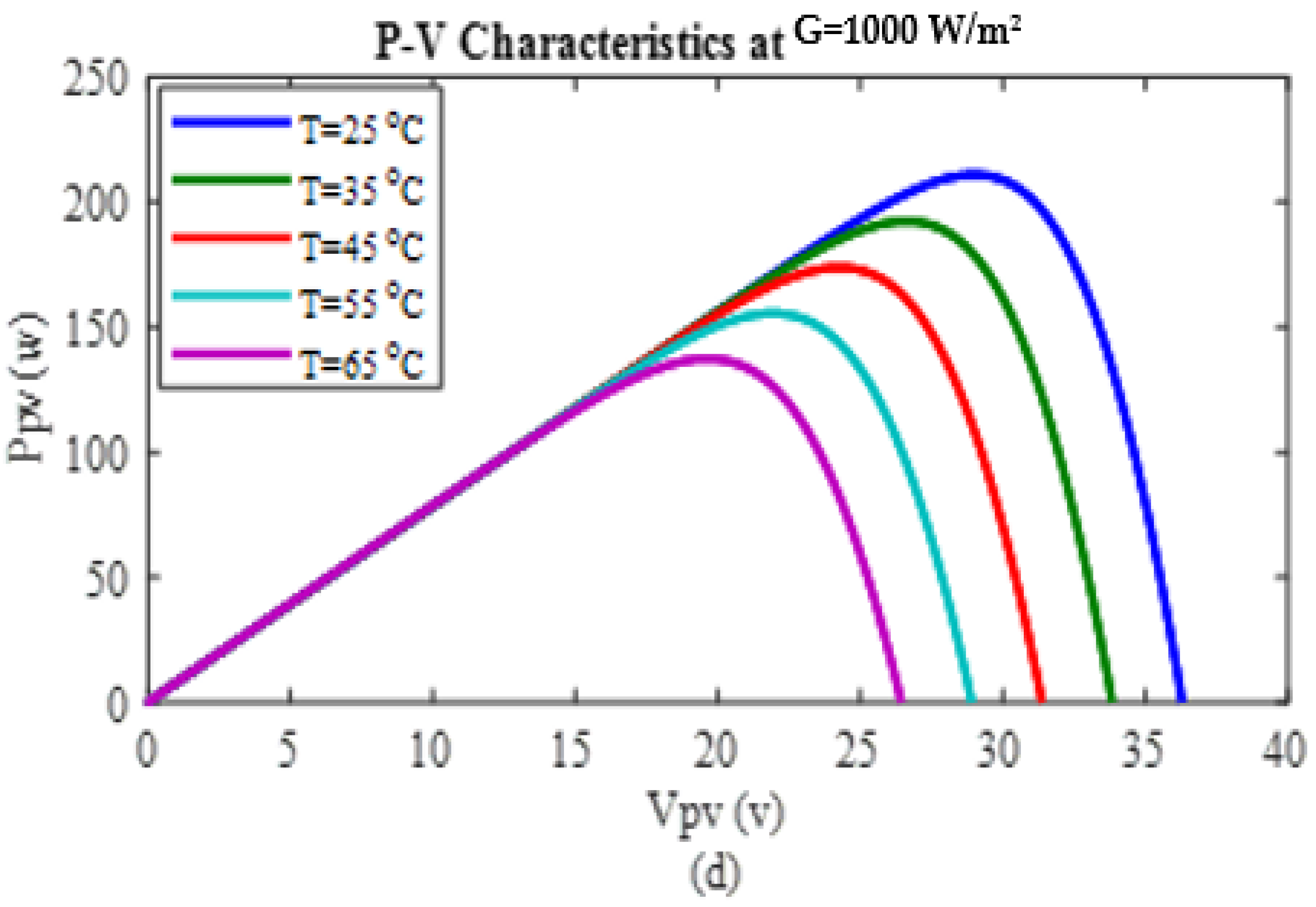
The V-I characteristics and V-P characteristics of the PV system are studied to show the nonlinear behavior of the PV system and the change of the position of the MPP under different irradiation and temperature. Figure 2 shows the PV system characteristics. It is evident from Figure 2a,c that the system has a unique maximum power point (MPP) at different irradiation and uniform temperature. The same for Figure 2b,d; the MPP changes with the change in temperature at uniform irradiation. Additionally, this change in the MPP reduces the efficiency due to the lower power conversion [35].

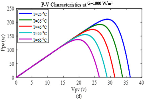
Figure 2. The PV characteristics (a). V-I characteristics at different G and T = 25 °C. (b) V-I characteristics at different T and $\mathrm{G}=1000\mathrm{W}/{\mathrm{m}}^2$. (c) P-V characteristics at different G and T = 25 °C. (d) P-V characteristics at different T and $\mathrm{G}=1000\mathrm{W}/{\mathrm{m}}^2$.

3. DC-DC Buck Converter

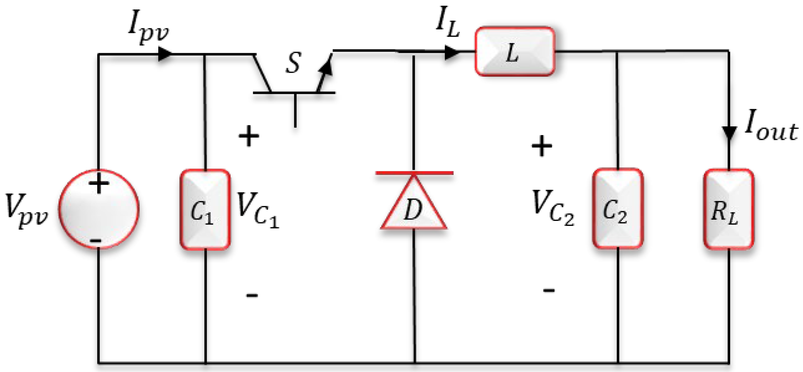
In the PV system, the DC–DC converter is used as a matching transformer. In case of a change in the load, the PV impedance changes, which in turn will change the MPP. So, by controlling the duty cycle entered to the gate of the switch (i.e., MOSFET, IGBT) of the converter, the system will operate at MPP regardless of the load change. A buck converter is a step-down converter used in the low voltage application, assuming the switch is operating at continuous conduction mode (CCM). A buck converter is used as a DC–DC converter in the underlying nonlinear system, as shown in Figure 3; there are two modes:

Figure 3. Buck converter equivalent circuit.

Mode 1: S is on and D is off:

$$\{\begin{array}{c}{I}_{C_1}=I_{pv}-I_L \\ V_L=V_{C_1}-V_{C_2} \\ I_{C_2}=I_L-I_{out} \end{array}$$

(7)

Mode 2: S is off and D is on:

$$\{\begin{array}{c}{I}_{C_1}=I_{pv} \\ V_L=-V_{C_2} \\ I_{C_2}=I_L-I_{out} \end{array}$$

(8)

In the steady-state condition, to find the average inductor voltage and capacitor current, the sum of Equations (7) and (8) yields:

$$\{\begin{array}{c}{I}_{C_1}=I_{pv}-I_L\mathbb{D} \\ V_L=V_{C_1}\mathbb{D}-V_{C_2} \\ I_{C_2}=I_L-I_{out} \end{array}$$

(9)

where $I_{C_1}$, $I_{C_2}$, $I_L$, $V_L$, $I_{out}$, $V_{C_1}$, $V_{C_2}$, and $\mathbb{D}$ are the input capacitor current, output capacitor current, inductor current, inductor voltage, converter output current, input capacitor voltage, output capacitor voltage, and duty cycle, respectively, with:

$$\{\begin{array}{c}{I}_{C_1}=C_1\frac{d{V}_{C_1}}{dt}\\ I_{C_2}=C_2\frac{d{V}_{C_2}}{dt}\\ V_L=L\frac{d{I}_L}{dt} \end{array}$$

(10)

Rewriting Equation (9), and with $I_{out}=\frac{V_{C_2}}{R_L},\mathbb{D}=u$, the dynamic model of the buck converter can be expressed as follows [36]:

$$\{\begin{array}{c}{\dot{V}}_{C_1}=\frac{1}{C_1}\left(I_{pv}-I_{L}u\right)\\ {\dot{I}}_L=\frac{1}{L}\left(V_{C_1}u-V_{C_2}\right)\\ {\dot{V}}_{C_2}=\frac{1}{C_2}\left(I_L-\frac{V_{C_2}}{R_L}\right) \end{array}$$

(11)

4. The Modified ADRC Design

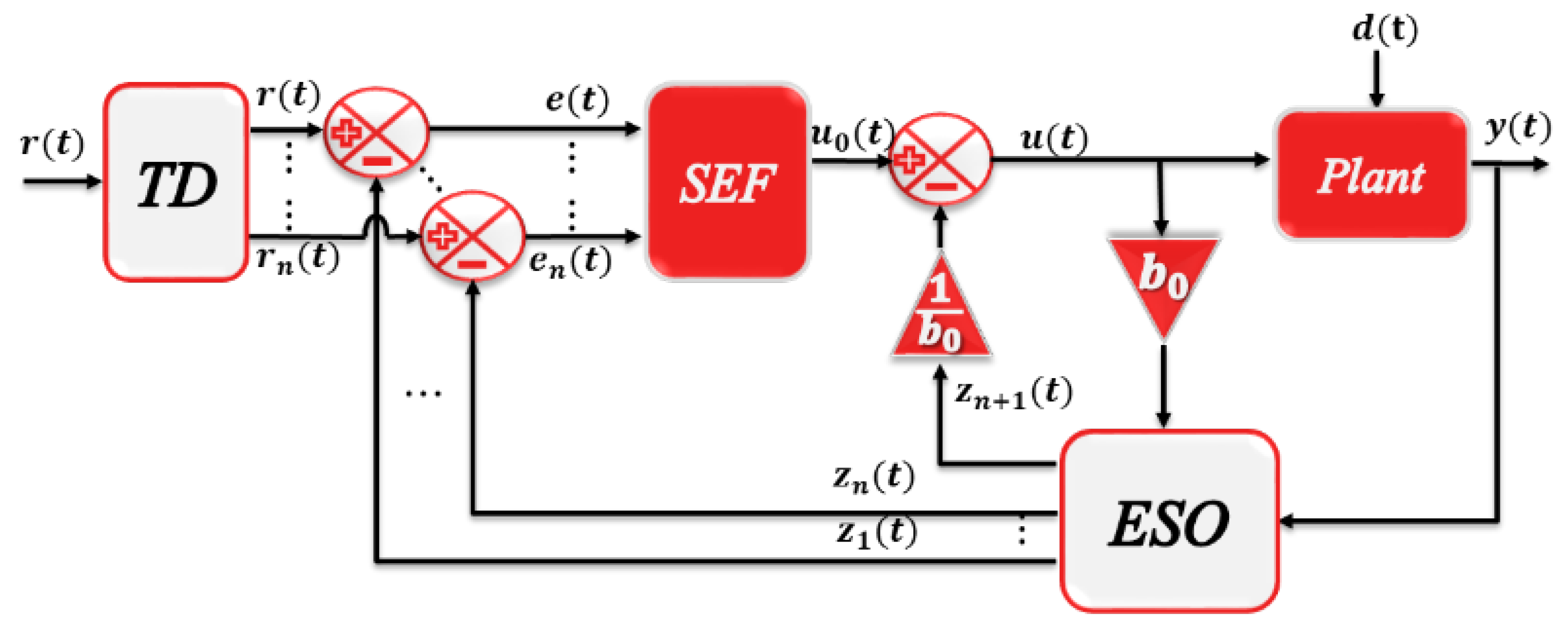
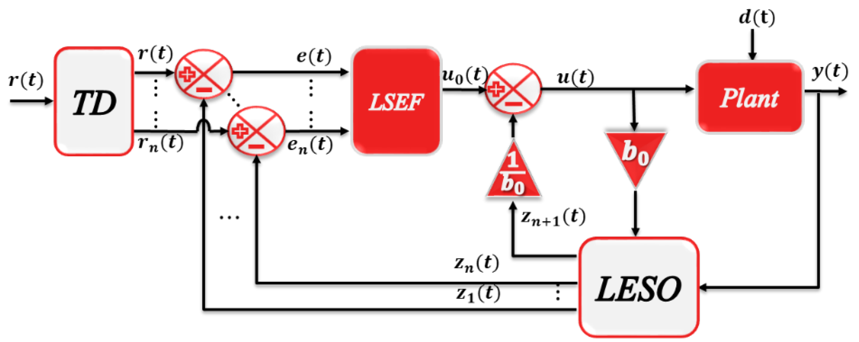
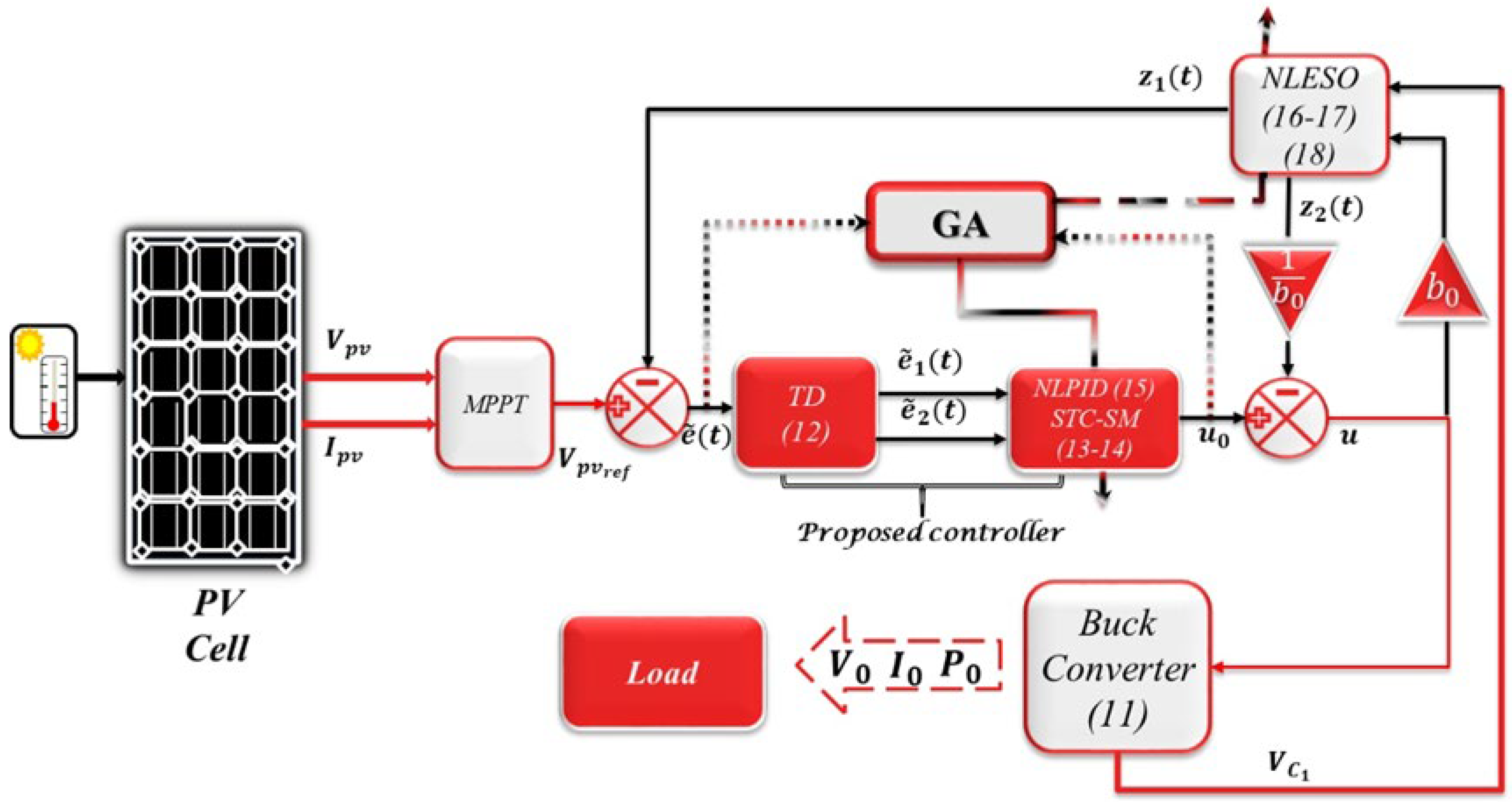
As mentioned previously, the ADRC is a control technique used to reject and eliminate disturbance and uncertainty in addition to stabilizing the overall system. Hence, in this paper, the ADRC for the system with a relative degree, $\rho =1$, is designed by incorporating the proposed tracking differentiator (TD) coupled with the proposed nonlinear state error feedback NLSEF to form the new nonlinear controller for the modified ADRC. Furthermore, the proposed NLESO and the new nonlinear controller form the modified ADRC. The general form of the proposed ADRC is shown in Figure 4. It consists of three parts that can be stated as follows:

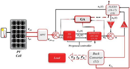
Figure 4. The MPPT–based proposed ADRC with the PV system with relative degree ($\rho =1)$, the numbers inside the parentheses in this figure indicate equation number in this paper.

4.1. The Proposed Tracking Differentiator

The dynamic equation of the proposed TD for relative degree $\rho =1$ is given as:

$$\{\begin{array}{c}{\dot{\tilde{e}}}_1={\tilde{e}}_2\\ {\dot{\tilde{e}}}_2=-a_1{R}^2\left(\frac{{\tilde{e}}_1-\tilde{e}}{\sqrt{1+{\left({\tilde{e}}_1-\tilde{e}\right)}^2}}\right)-a_{2}R{\tilde{e}}_2\end{array}$$

(12)

where, ${\tilde{e}}_1$, ${\tilde{e}}_2$ are the tracking errors and their derivative, respectively;$\tilde{e}$ is the input error to the TD; $R$ is a positive tuning parameter; and $a_1$ and $a_2^{}$ are tuning parameters. In the proposed TD, the sigmoid function (i.e., “Elliott squash function” is used instead of the $sign$ function in the classical TD of [26]. Moreover, in the proposed TD, the error is used as an input to the tracking differentiator and the output is a smooth signal of the error and its derivative.

4.2. The Proposed Nonlinear Controllers

In this section, the proposed controller utilized in this work is introduced and stated as follows:

4.2.1. The Proposed Super Twisting Sliding Mode Controller (STC-SM)

Recently, the classical super twisting controller (CST-SMC) is widely used in different fields, to avoid the chattering problem [37,38]. Thus, in this paper, a new STC-SM is proposed to enhance the avoidance of STC-SM against the chattering in the control signal. The proposed STC-SM can be expressed as follows:

$$\varsigma =\mathsf{\kappa }{\tilde{e}}_1+{\dot{\tilde{e}}}_1$$

(13)

$$u_{0_{STC-SM}}=\kappa {\left|\varsigma \right|}^{𝓅}sign\left(\varsigma \right)+\xi tanh\left(\frac{\varsigma }{\delta }\right)$$

(14)

where $\varsigma$ is the sliding surface; ${\tilde{e}}_1$ and ${\dot{\tilde{e}}}_1$ are the tracking errors and their derivative, respectively; $\xi$ is the sliding coefficient; and $𝓅$ and $\delta$ are positive parameters to be tuned, $0<𝓅<1$, $\delta >0$.

4.2.2. The Proposed Nonlinear PID—Tracking Differentiator (NLPID-TD)

The NLPID is the modified nonlinear version of the linear PID (LPID) controller. The NLPID-TD controller is an aggregation of the TD and the NLPID controller, which can be expressed as follows:

$$\{\begin{array}{c}{u}_1=\frac{k_1}{1+\mathit{exp}\left({\tilde{e}}_1{}^2\right)} {\left|{\tilde{e}}_1\right|}^{{\alpha }_1}sign\left({\tilde{e}}_1\right) \\ u_2=\frac{k_2}{1+\mathit{exp}\left({\dot{\tilde{e}}}_1{}^2\right)} {\left|{\dot{\tilde{e}}}_1\right|}^{{\alpha }_2}sign\left({\dot{\tilde{e}}}_1\right) \\ u_3=\frac{k_3}{1+exp\left(\int {\tilde{e}}_1{}^2\right)} {\left|{\tilde{e}}_1\right|}^{{\alpha }_3}sign\left({\displaystyle \int }{\tilde{e}}_{1}dt\right)\\ u_{0_{NLPID}}=u_1+u_2+u_3\end{array}$$

(15)

where $k_1,k_2,k_3,{\alpha }_1,{\alpha }_2,\mathrm{and}{\alpha }_3$ are tuning design parameters and ${\dot{\tilde{e}}}_1={\tilde{e}}_2$. Moreover, ${\alpha }_1,{\alpha }_2,\mathrm{and}{\alpha }_3<1$ to ensure the error functions ${\left|\tilde{e}\right|}^{{\alpha }_1},$ ${\left|{\tilde{e}}_1\right|}^{{\alpha }_2} \mathrm{and}{\left|{\dot{\tilde{e}}}_1\right|}^{{\alpha }_3}$ are sensitive to small error values. This indicates that $u_1$ uses the racking error, which is the proportional term, but a nonlinear one, while $u_2$ uses the derivative of the tracking error, which casts the derivative term. Finally, the integral of the tracking error is issued in $u_3$ to form the integral term. These three terms are nonlinear. The weighted combination of these three terms is denoted as $u_0$.

4.3. The Proposed NLESO

To properly estimate the “total disturbance” and eliminate its effect on the system, an NLESO is proposed. The dynamic equations of the proposed NLESO are given as:

$$\{\begin{array}{c}{\dot{z}}_1=z_2+b_{0}u+{\beta }_1{\widehat{e}}_1 \\ {\dot{z}}_2={\beta }_2{\widehat{e}}_2 \end{array}$$

(16)

$$\{\begin{array}{c}{\widehat{e}}_1=sign\left(e_1\right){\left|e_1\right|}^{a_1}+𝒜e_1 \\ {\widehat{e}}_2=sign\left(e_1\right){\left|e_1\right|}^{\raisebox{1ex}{$a_1$}\!\left/ \!\raisebox{-1ex}{$2$}\right.}+𝒜e_1\end{array}$$

(17)

where $e_1$ = $V_{C_1}-z_1$; $e_1$ is the estimation error; $z_1$ is the estimation state of $V_{C_1}$; ${\widehat{e}}_1$ and ${\widehat{e}}_2$ are nonlinear functions; $a_1$ is a tuning parameter that should be less than 1; $\mathcal{A}$ is a tuning parameter; ${\beta }_1$ and ${\beta }_2$ are the observer gain parameters, and they are selected in such a way that the characteristic polynomial $s^2+{\beta }_{1}s+{\beta }_2={\left({\omega }_0+s\right)}^2$ is Hurwitz [39,40]; and ${\omega }_0$ is the NLESO bandwidth. Another scheme of the NLESO is also proposed in this paper and it is expressed as follows:

$$\{\begin{array}{c}{\dot{z}}_1=z_2+b_{0}u+{\beta }_1{\widehat{e}}_1 \\ {\dot{z}}_2={\beta }_2{\widehat{e}}_2\\ {\widehat{e}}_1=sign\left(e_1\right){\left|e_1\right|}^{a_1}+e_1\\ {\widehat{e}}_2=sign\left(e_1\right){\left|e_1\right|}^{2a_1-1}+e_1\end{array}$$

(18)

where $0.55<a_1<1$ is a positive tuning parameter. The proposed ADRC with the nonlinear model of the PV system is shown in Figure 4.

5. Stability of the Closed-Loop System

In this section, closed-loop stability is introduced using the Lyapunov stability approach. Firstly, let $x_1=V_{C_1}$, then, Equation (11) can be rewritten as:

$$\{\begin{array}{c}{\dot{x}}_1=\frac{1}{C_1}\left(I_{pv}-I_{L}u\right)\\ y=x_1\end{array}$$

(19)

With $I_{pv}=\frac{V_{pv}}{R_{pv}}$ and $V_{pv}=V_{C_1}$, Equation (19) can be rewritten as:

$$\{\begin{array}{c}{\dot{x}}_1=\frac{1}{C_1{R}_{pv}}{x}_1-\frac{I_L}{C_1}u+d\\ y=x_1\end{array}$$

(20)

Adding $\pm b_{0}u$ to Equation (20) obtains:

$$\{\begin{array}{c}{\dot{x}}_1=f\left(x_1,I_L,t\right)+b_{0}u+d\\ y=x_1\end{array}$$

(21)

where $f\left(x_1,I_L,t\right)=\frac{1}{C_1{R}_{pv}}{x}_1-\frac{I_L}{C_1}u-b_{0}u$. Let:

$$x_3=f\left(x_1,I_L,t\right)+d$$

(22)

Sub. Equation (22) in Equation (21) and one obtains:

$$\{\begin{array}{c}{\dot{x}}_1=x_2+b_{0}u\\ y=x_1\end{array}$$

(23)

where $f\left(x_1,I_L,d,t\right)$ is the system dynamic, $d$ is the exogenous disturbance, and $x_2$ is the total disturbance. Now, differentiate Equation (23), which yields:

$${\dot{x}}_3=\dot{f}\left(x_1,I_L,d,t\right)+\dot{d}$$

(24)

Assumption 1. 

The two schemes of the NLESO given in Equations (16)–(18) estimate the states of the nonlinear system completely.

$$\underset{t\to \infty }{\lim }{e}_1=0$$

Theorem 1. 

Based on Assumption 1, the proposed NLESO estimates the total disturbance and the estimated error$e_1=x_1-z_1$ is asymptotically converged to zero as $t\to \infty$ if the observer gains ${\beta }_1$ and ${\beta }_2$ are designed so that the $Q$ matrix is negative definite.

Proof. 

The estimated error can be expressed as:

$$e_i=x_i-z_i$$

(25)

where $i=\left\{1,\cdots ,\rho +1\right\},$ $e_1$ is the estimated error, $z_1$ is the estimated state of $x_1$, and $\rho$ is the relative degree which is equal to 1. Differentiating Equation (25) obtains:

$${\dot{e}}_i={\dot{x}}_i-{\dot{z}}_i$$

(26)

Let $\ell =x_2$ describe the total disturbance. The substitution of the first term of Equation (23) and Equation (16) or Equation (18) into Equation (26) yields:

$$\{\begin{array}{c}{\dot{e}}_1=x_2-z_2-{\beta }_1{\widehat{e}}_1\\ {\dot{e}}_2=\dot{\ell }-{\beta }_2{\widehat{e}}_2 \end{array}$$

(27)

Expressing Equation (27) in matrix form:

$$\dot{e}={\mathsf{A}}_{0}e+{\mathsf{A}}_d\dot{\ell }$$

(28)

Let ${\widehat{e}}_1={\mathsf{{\rm K}}}_1\left(e_1\right)\mathrm{and}{\widehat{e}}_2={\mathsf{{\rm K}}}_2\left(e_1\right)$. Then:

$${\mathsf{A}}_0=\left[\begin{array}{cc}-{\beta }_1{{\rm K}}_1\left(e_1\right)& 0\\ -{\beta }_2{{\rm K}}_2\left(e_1\right)& 1\end{array}\right],{\mathsf{A}}_d=\left[\begin{array}{c}0\\ 1\end{array}\right],\dot{e}=\left[\begin{array}{cc}{\dot{e}}_1& {\dot{e}}_2\end{array}\right],e=\left[\begin{array}{cc}{e}_1& e_2\end{array}\right]$$

To prove the convergence of the proposed NLESO, Lyapunov stability is applied [41]. Let us assume the Lyapunov function $V_{NLESO}=\frac{1}{2}{e}^{T}e$. Then, ${\dot{V}}_{NLESO}=e^T\dot{e}$, for $\rho =1$:

$${\dot{V}}_{NLESO}=\left[\begin{array}{cc}{e}_1& e_2\end{array}\right]\left[\begin{array}{cc}-{\beta }_1{\mathsf{{\rm K}}}_1\left(e_1\right)& 0\\ -{\beta }_2{\mathsf{{\rm K}}}_2\left(e_1\right)& 1\end{array}\right]\left[\begin{array}{c}{e}_1\\ e_2\end{array}\right]+\dot{\ell }$$

Assumption 2 

([42]).The total disturbance$\ell$should satisfy the following conditions:

• $\ell$and$\dot{\ell }$ are bounded, which, $\underset{0\le t\le \infty }{\mathit{sup}}\ell \le c_1$and $\underset{0\le t\le \infty }{\mathit{sup}}\dot{\ell }\le c_2$
• $\ell$and $\dot{\ell }$ are constant at the steady-state, which, $\underset{t\to \infty }{\lim }\ell =c_3$ and $\underset{t\to \infty }{\lim }\dot{\ell }\le 0$

Where $c_1,$ $c_2,$ and $c_3$ are positive constants.

Based on Assumption 2, $\dot{\ell }$ converges to zero as $t\to \infty$, then:

$${\dot{V}}_{NLESO}=\left[\begin{array}{cc}{e}_1& e_2\end{array}\right]\left[\begin{array}{cc}-{\beta }_1{\mathsf{{\rm K}}}_1\left(e_1\right)& 0\\ -{\beta }_2{\mathsf{{\rm K}}}_2\left(e_1\right)& 1\end{array}\right]\left[\begin{array}{c}{e}_1\\ e_2\end{array}\right]$$

The system is asymptotically stable when the $Q$ matrix is a negative definite. To verify whether the $Q$ matrix is negative definite, Routh stability is exploited. The characteristic equation for matrix $Q$ can be expressed as:

$$\left|\lambda \mathrm{I}-Q\right|=0,\left|\begin{array}{cc}\lambda +{\beta }_1{\mathsf{{\rm K}}}_2\left(e_1\right)& -1\\ {\beta }_2{\mathsf{{\rm K}}}_2\left(e_1\right)& \lambda \end{array}\right|=0$$

Then, from Routh stability criteria:

$$\begin{array}{ccc}1& {\mathsf{\beta }}_2{\mathrm{K}}_2\left({\mathrm{e}}_1\right)& 1\\ {\mathsf{\beta }}_1{\mathrm{K}}_1\left({\mathrm{e}}_1\right)& 0& {\mathsf{\beta }}_1{\mathrm{K}}_1\left({\mathrm{e}}_1\right)\\ \frac{{\mathsf{\beta }}_2{\mathsf{{\rm K}}}_2\left({\mathrm{e}}_1\right){\mathsf{\beta }}_1{\mathsf{{\rm K}}}_1\left({\mathrm{e}}_1\right)}{{\mathsf{\beta }}_1{\mathsf{{\rm K}}}_1\left({\mathrm{e}}_1\right)}={\mathsf{\beta }}_2{\mathsf{{\rm K}}}_2\left({\mathrm{e}}_1\right)& 0& \frac{{\mathsf{\beta }}_2{\mathsf{{\rm K}}}_2\left({\mathrm{e}}_1\right){\mathsf{\beta }}_1{\mathsf{{\rm K}}}_1\left({\mathrm{e}}_1\right)}{{\mathsf{\beta }}_1{\mathsf{{\rm K}}}_1\left({\mathrm{e}}_1\right)}={\mathsf{\beta }}_2{\mathsf{{\rm K}}}_2\left({\mathrm{e}}_1\right)\end{array}$$

$${\lambda }^2+{\beta }_1{\mathsf{{\rm K}}}_1\left(e_1\right) \lambda +{\beta }_2{\mathsf{{\rm K}}}_2\left(e_1\right)=0$$

$${\beta }_1{\mathsf{{\rm K}}}_1\left(e_1\right)>0, {\beta }_1>0, {\beta }_2{\mathsf{{\rm K}}}_2\left(e_1\right)>0, {\beta }_2>0$$

Then, $Q$ is negative definite if the observer gains ${\beta }_1$ and ${\beta }_2>0$. Based on this, it can be concluded that the NLESO is asymptotically stable. □

Now, the error dynamic of the closed-loop system can be written as:

$$\tilde{e}=r-z_1$$

(29)

Differentiating Equation (29) yields:

$$\dot{\tilde{e}}=\dot{r}-{\dot{z}}_1$$

(30)

Simplifying Equation (30) obtains:

$$\dot{\tilde{e}}=-z_2-b_{0}u$$

(31)

Assumption 3. 

The tracking differentiator in Equation (12) tracks the reference error signal with a very small error that approaches zero and with $\dot{\tilde{e}}=0$

.

$$\underset{t\to \infty }{\lim }\left|{\tilde{e}}_1-\tilde{e}\right|=0$$

Theorem 2. 

Given the nonlinear system given in Equation(14) and the modified ADRC, then based on Assumptions 1–3, the closed-loop system is stable if $\left\{{𝒦}_1\left({\tilde{e}}_1\right){\tilde{e}}_1, {𝒦}_2\left({\tilde{e}}_2\right){\tilde{e}}_2\right\}$is chosen in such a way that the $Q$matrix is negative definite and that the characteristics equation ${\lambda }^2+\lambda \left({\acute{𝒦}}_1+{\acute{𝒦}}_2\right)+\acute{\stackrel{´}{{𝒦}_1}\stackrel{´}{{𝒦}_2}}=0$. is Hurwitz.

Proof. 

With $u=u_0-\frac{z_2}{b_0}$, Equation (31) can be rewritten as:

$$\dot{\tilde{e}}=-z_2-b_0\left[u_0-\frac{z_2}{b_0}\right]$$

(32)

Simplifying Equation (32) obtains:

$$\dot{\tilde{e}}=-b_0{u}_0$$

(33)

Substituting the NLPID Equation (15) or STC-SM Equation (14) in Equation (33), one obtains:

Remark 1. 

The $u_3$term in the proposed NLPID given in Equation(15) could be removed because the extended state$z_2$approaches the generalized disturbance $\ell$as $t\to \infty$and converts the system Equation (19) into a chain of integrators. So, there is no need for the integrator term $u_3$. Therefore, the NLPD will be used in this work and expressed as follows:

$$\{\begin{array}{c}{u}_{0_{NLPD}}=u_1+u_2 \\ u_1=\frac{k_1}{1+\mathit{exp}\left({\tilde{e}}_1{}^2\right)} {\left|{\tilde{e}}_1\right|}^{{\alpha }_1}sign\left({\tilde{e}}_1\right) \\ u_2=\frac{k_2}{1+\mathit{exp}\left({\dot{\tilde{e}}}_1{}^2\right)} {\left|{\dot{\tilde{e}}}_1\right|}^{{\alpha }_2}sign\left({\dot{\tilde{e}}}_1\right) \end{array}$$

(34)

Sub. Equation (34) in Equation (33) to obtain:

$$\dot{\tilde{e}}=-b_0\left[u_1\left({\tilde{e}}_1\right)+u_2\left({\tilde{e}}_2\right)\right]$$

(35)

Assumption 3. 

Let ${\mathcal{K}}_i\left({\tilde{e}}_i\right)=$$\frac{k_i}{1+exp\left({\tilde{e}}_i{}^2\right)}$, $i\in \{1,2\}$, and ${\alpha }_1$,${\alpha }_2$approach unity. According to that, the term $\left|\mathbb{S}\right|sign\left(\mathbb{S}\right)$in Equation (35) is approximately equal to $\mathbb{S}$. So, based on Assumption 3, Equation (35) can be rewritten as:

$$\dot{\tilde{e}}=-b_0\left[{\mathcal{K}}_1\left({\tilde{e}}_1\right){\tilde{e}}_1+{\mathcal{K}}_2\left({\tilde{e}}_2\right){\tilde{e}}_2\right]$$

(36)

Now, expressing Equation (36) in matrix form:

$$\dot{\tilde{e}}=A_{C_{NLPD}}\tilde{e}$$

where $A_{C_{NLPD}}=\left[\begin{array}{cc}-{\acute{\mathcal{K}}}_1& -{\acute{\mathcal{K}}}_2\end{array}\right]$, $\tilde{e}=\left[\begin{array}{c}{\tilde{e}}_1\\ {\tilde{e}}_2\end{array}\right]$, ${\acute{\mathcal{K}}}_i=b_0{\mathcal{K}}_i\left({\tilde{e}}_i\right),i\in \left\{1,2\right\}$. Now, the Lyapunov function is used to check the stability of the closed-loop system, let $V_{cl}=\frac{1}{2}{\tilde{e}}^T\tilde{e}$, then, ${\dot{V}}_{cl}={\tilde{e}}^T\dot{\tilde{e}}$:

$${\dot{V}}_{cl}=\left[\begin{array}{cc}{\tilde{e}}_1& {\tilde{e}}_2\end{array}\right]\left[\begin{array}{cc}-{\acute{\mathcal{K}}}_1& -{\acute{\mathcal{K}}}_2\end{array}\right]\left[\begin{array}{c}{\tilde{e}}_1\\ {\tilde{e}}_2\end{array}\right]$$

The characteristic equation for the matrix $Q$ is found using the Routh stability criterion to find whether the system is stable or not.

$$\left|\lambda \mathrm{I}-\mathrm{Q}\right|=0,\left|\begin{array}{cc}\lambda & 0\\ 0& \lambda \end{array}\right|-\left|\begin{array}{cc}-{\acute{\mathcal{K}}}_1& 0\\ 0& -{\acute{\mathcal{K}}}_2\end{array}\right|$$

$${\lambda }^2+\lambda \left({\acute{\mathcal{K}}}_1+{\acute{\mathcal{K}}}_2\right)+\stackrel{´}{\acute{{\mathcal{K}}_1}\acute{{\mathcal{K}}_2}}=0$$

$$\begin{array}{ccc}{\mathsf{\lambda }}^2& 1& \acute{{\mathcal{K}}_1}\acute{{\mathcal{K}}_2}\\ \mathsf{\lambda }& {\acute{\mathcal{K}}}_1+{\acute{\mathcal{K}}}_2& 0\\ {\mathsf{\lambda }}^0& \frac{\left({\acute{\mathcal{K}}}_1+{\acute{\mathcal{K}}}_2\right)\acute{{\mathcal{K}}_1}\acute{{\mathcal{K}}_2}}{{\acute{\mathcal{K}}}_1+{\acute{\mathcal{K}}}_2}=\acute{{\mathcal{K}}_1}\acute{{\mathcal{K}}_2}& 0\end{array}$$

$$\acute{{\mathcal{K}}_1}\acute{{\mathcal{K}}_2}>0\Rightarrow {\mathcal{K}}_1>0\mathrm{or}{\mathcal{K}}_2>0$$

Thus, the matrix $Q$ is negative definite and the system is stable if the nonlinear function gain ${\acute{\mathcal{K}}}_1$ and ${\acute{\mathcal{K}}}_2$ satisfy the condition above. □

Now with the STC-SM, the substitution of Equation (14) into Equation (33) yields:

$$\dot{\tilde{e}}=-b_0\left[\kappa {\left|\varsigma \right|}^{𝓅}sign\left(\varsigma \right)+\xi tanh\left(\frac{\varsigma }{\delta }\right)\right]$$

(37)

where $\varsigma =\mathsf{\kappa }{\tilde{e}}_1+{\dot{\tilde{e}}}_1$.

As mentioned previously, the Lyapunov function is used to check the stability of the closed-loop system. Let $V_{cl}=\frac{1}{2} {\varsigma }^T\varsigma$, then, ${\dot{V}}_{cl}={\varsigma }^T\dot{\varsigma }$, with $\dot{\varsigma }=u_{0_{STC-SM}}$, then:

$${\dot{V}}_{cl}={\varsigma }^T\left[-\kappa {\left|\varsigma \right|}^{\rho }sign\left(\varsigma \right)-\xi tanh\left(\frac{\varsigma }{\delta }\right)\right]$$

$$\backslash {\dot{V}}_{cl}=-\kappa {\left|\varsigma \right|}^{\rho +1}sign\left(\varsigma \right)-\varsigma \xi tanh\left(\frac{\varsigma }{\delta }\right)$$

$$\therefore {\dot{V}}_{cl}<0 if \kappa \mathrm{and}\xi >0$$

Then, the overall system is stable. □

6. Simulation Results

In this section, the simulation results of the PV-MPPT with the modified ADRC are presented. The design and the obtained simulation results of the PV-MPPT were performed using a MATLAB/SIMULINK environment. Moreover, to investigate the robustness and accuracy of the proposed method, three case studies have been applied and stated in sequence as follows:

• Case study one: Irradiation changes with constant temperature at standard temperature conditions (STC).
• Case study two: Temperature changes with constant irradiation at standard temperature conditions (STC).
• Case study three: Load changes in both irradiation and temperature at standard temperature conditions (STC).

In addition, the PV cell parameters and the DC–DC converter parameters are presented in this section. Table 1 and Table 2 represent the sampled parameters of the PV cell and buck converter. Correspondingly, a multi-objective output performance index (OPI) is used and expressed as follows:

$$OPI={𝒲}_1\times \frac{ITAE}{{𝒩}_1}+{𝒲}_2\times \frac{IAU}{{𝒩}_2}+{𝒲}_3\times \frac{ISU}{{𝒩}_3}$$

(38)

where ${𝒲}_1,{𝒲}_2, \mathrm{and} {𝒲}_3$ are the weighting factors that satisfy ${𝒲}_1+{𝒲}_2+{𝒲}_3$= 1 and are set to ${𝒲}_1=0.5,{𝒲}_2=0.4 \mathrm{and} {𝒲}_3=0.1$. ${𝒩}_1,{𝒩}_2, \mathrm{and} {𝒩}_3$ are the nominal values of the individual objective functions. Their values are set to ${𝒩}_1=179.197287, {𝒩}_2=5121.329977,\mathrm{and} {𝒩}_3=47.850042$. The description and the mathematical representation of the utilized performance indices are listed in Table 3. Furthermore, the aforementioned OPI is used in all the case studies mentioned previously. Finally, all the methods utilized in this work are summarized in Table 4.

Table 1. PV-cell sampled parameters [43].

Parameters	Description	Value	Unit
$K_0$	Boltzmann constant	$1.380\times {10}^{-23}$	$\mathrm{J}/\mathrm{K}$
$q_0$	Electron charge	$1.602\times {10}^{-19}$	$\mathrm{C}$
$I_{SC}$	Short circuit current at STC	$7.84\times {10}^0$	$\mathrm{A}$
$V_{OC}$	Open circuit voltage at STC	$36.3\times {10}^0$	$\mathrm{V}$
$K_v$	Temperature voltage constant	$18\times {10}^{-1}$	$\mathrm{V}/\mathrm{K}\%$
$K_i$	Temperature current constant	$0.00175$	$\mathrm{A}/\mathrm{K}\%$
$A_{diode}$	Diode ideality factor	$1.3$	$\mathrm{Unitless}$
$T_{ref}$	Temperature at STC	$298$	$\mathrm{K}$
$G_{ref}$	Irradiation at STC	$1000$	$\mathrm{w}/{\mathrm{m}}^2$
$E_{g_0}$	Band-gap energy	$1.12$	$\mathrm{Ev}$
$R_s$	Series resistance	$0.2656$	$\mathsf{\Omega }$
$R_P$	Parallel resistance	$1000$	$\mathsf{\Omega }$
$N_s$	Number of cells connected in series	$60$	$\mathrm{Unitless}$
$N_P$	Number of cells connected in parallel	$1$	$\mathrm{Unitless}$
$N_{ms}$	Number of modules connected in series	$10$	$\mathrm{Unitless}$

Table 2. DC–DC buck converter parameters.

Parameters	Description	Value	Unit
$C_1$	The input capacitor	$350$	$mF$
$C_2$	The output capacitor	$35$	$mF$
$L$	Inductor	$270$	$mH$
$R_L$	Load resistance	$1.6$	$\mathsf{\Omega }$
$f_s$	Switching frequency	$50$	$H\mathcal{z}$

Table 3. Mathematical representation of the performance indices.

Performance Index	Description	Mathematical Representation
$ITAE$	Integral Time Absolute Error	${{\displaystyle \int }}_0^{tf}t\left|e\left(t\right)\right|dt$
$IAU$	Integral Absolute of the control signal	${{\displaystyle \int }}_0^{tf}\left|u\left(t\right)\right|dt$
$ISU$	Integral Square of the control signal	${{\displaystyle \int }}_0^{tf}u{\left(t\right)}^{2}dt$

Table 4. A summary of the ADRC schemes.

Scheme	ADRC Parts
	TD	SEF	ESO
LADRC	$-$	$u_{LPID}=k_p\tilde{e}+k_i{\int }_0^T\tilde{e} dt+k_d\frac{d\tilde{e}}{dt};u=u_{0_{LPID}}-z_2/b_0$  $\mathrm{Where}{\mathrm{k}}_{\mathrm{p}},{\mathrm{k}}_{\mathrm{i}},{\mathrm{k}}_{\mathrm{d}}$ are the proportional, integral, and derivative gains, respectively.	The LESO can be expressed as follows: $\{\begin{array}{l}{\dot{z}}_1=z_2+b_{0}u+{\beta }_1\left(e_1\right)\\ {\dot{z}}_2={\beta }_2\left(e_1\right)\end{array}$
ADRC	$-$	The NLSEF of [33] can be expressed as follows: $\{\begin{array}{l}fal\left({\tilde{e}}_1,{\alpha }_1,{\delta }_1\right)=\{\begin{array}{c}{\tilde{e}}_1/\left({\delta }_1{}^{1-{\alpha }_1}\right), x\le {\delta }_1\\ {\left|{\tilde{e}}_1\right|}^{{\alpha }_1}sign\left({\tilde{e}}_1\right), x>{\delta }_1\end{array}\\ u_0=fal\left({\tilde{e}}_1,{\alpha }_1,{\delta }_1\right) \\ u_1=u_{0_{NLSEF}}-z_2/b_0\end{array}$
IADRC	$-$	The INLSEF of [44] can be expressed as: $\{\begin{array}{c}{u}_1=\frac{k_1}{1+exp\left({\tilde{e}}^2\right)}{\left|\tilde{e}\right|}^{{\alpha }_1}sign\left(\tilde{e}\right) \\ u_2=\frac{k_2}{1+exp\left(\int {\tilde{e}}^{2}dt\right)}{\left|{\displaystyle \int }\tilde{e}dt\right|}^{{\alpha }_2}sign\left({\displaystyle \int }\tilde{e}dt\right)\\ u_{0_{INLSEF}}=u_1+u_2; u=u_{INLSEF}-z_2/b_0 \end{array}$	The SMESO of [45] can be expressed as:$\{\begin{array}{c}{\dot{z}}_1\left(t\right)=z_2\left(t\right)+{\beta }_1\left(k\left(e_1\left(t\right)\right)e_1\left(t\right)\right)\\ {\dot{z}}_{\rho +1}\left(t\right)={\beta }_{\rho +1}\left(k\left(e_1\left(t\right)\right)e_1\left(t\right)\right) \\ k\left(e_1\left(t\right)\right)=k_{\alpha }{\left|e_1\right|}^{\alpha -1}+k_{\beta }{\left|e_1\right|}^{\beta }\end{array}$  $\mathrm{where}k\left(e_1\left(t\right)\right)$$\mathrm{is}\mathrm{a}\mathrm{nonlinear}\mathrm{function}\mathrm{and}\alpha \mathrm{and} \beta$$\mathrm{are}\mathrm{positive}\mathrm{tuning}\mathrm{parameters}\mathrm{that}\mathrm{must}\mathrm{be}\mathrm{less}\mathrm{than}1.k_{\alpha } \mathrm{and} k_{\beta }$ are the nonlinear function gains and are tuning parameters.
STC-ADRC	Equation (12)	The proposed STC-SM of Equations (12) and (13).	Proposed NLSEO of Equations (16) and (17).
NLPD-ADRC	Equation (12)	The proposed NLPD of Equation (33).	Proposed NLSEO of Equation (18).

i.

Case study one. Irradiation changes with constant temperature at standard temperature conditions (STC).

In this test, different irradiations were applied at different times and considered an exogenous disturbance. Moreover, a step function was used for both reference and irradiation changes. Moreover, the parameters of all the methods used after the tuning are shown in Table 5, Table 6, Table 7, Table 8 and Table 9.

Table 5. Th/4e LADRC parameters.

ADRC Unit	Parameter	Value	Parameter	Value
LPID	$k_p$	$0.088$	$k_i$	1 × 10−9
	$k_d$	$0.088$	$\delta$	$10.326$
LESO	${\beta }_1$	$1.78$	${\beta }_2$	$0.792100$

Table 6. The ADRC parameters.

ADRC Unit	Parameter	Value	Parameter	Value
NLSEF	${\alpha }_1$	$0.7729$	${\delta }_1$	$0.3949$
LESO	${\beta }_1$	$102.3$	${\beta }_2$	$2616.3225$
	$b_0$	$7.375714$	$-$	$-$

Table 7. The IADRC parameters.

ADRC Unit	Parameter	Value	Parameter	Value
INLSEF (NLPI)	$k_{11}$	$1.524$	$k_2$	$0.6168$
	$k_{12}$	$2.456$	${\mu }_2$	$0.0222$
	${\mu }_1$	$3.0164$	${\alpha }_2$	$0.9593$
	${\alpha }_1$	$0.9615$	$\delta$	$0.8865$
SMESO	${\beta }_1$	$138.18$	${\beta }_2$	$4773.4281$
	$k_{\alpha }$	$0.9874$	$k_{\beta }$	$0.3604$
	$\alpha$	$0.3506$	$\beta$	$0.2225$
	$b_0$	$11.176$	$-$	$-$

Table 8. The NLPD-ADRC parameters.

ADRC Unit	Parameter	Value	Parameter	Value
NLPD	$k_1$	$6.1775$	$k_2$	$8.339$
	${\alpha }_1$	$0.8391$	${\alpha }_2$	$0.8015$
TD	$R$	$55.38$	$a_2$	$7.842$
	$a_1$	$0.142$	$-$	$-$
NLESO	${\beta }_1$	$114.64$	${\beta }_2$	$3285.582400$
	$a_1$	$0.6129$	$b_0$	$6.305714$

Table 9. STC-ADRC parameters.

ADRC Unit	Parameter	Value	Parameter	Value
STC-SM	$\kappa$	$0.6704$	$\xi$	$0.74115$
	$𝓅$	$0.3035$	$\delta$	$0.6697$
TD	$R$	$55.38$	$a_2$	$7.842$
	$a_1$	$0.142$	$-$	$-$
NLESO	${\beta }_1$	$169.6$	${\beta }_2$	$7191.04$
	$a_1$	$0.5563$	$b_0$	$9.521429$

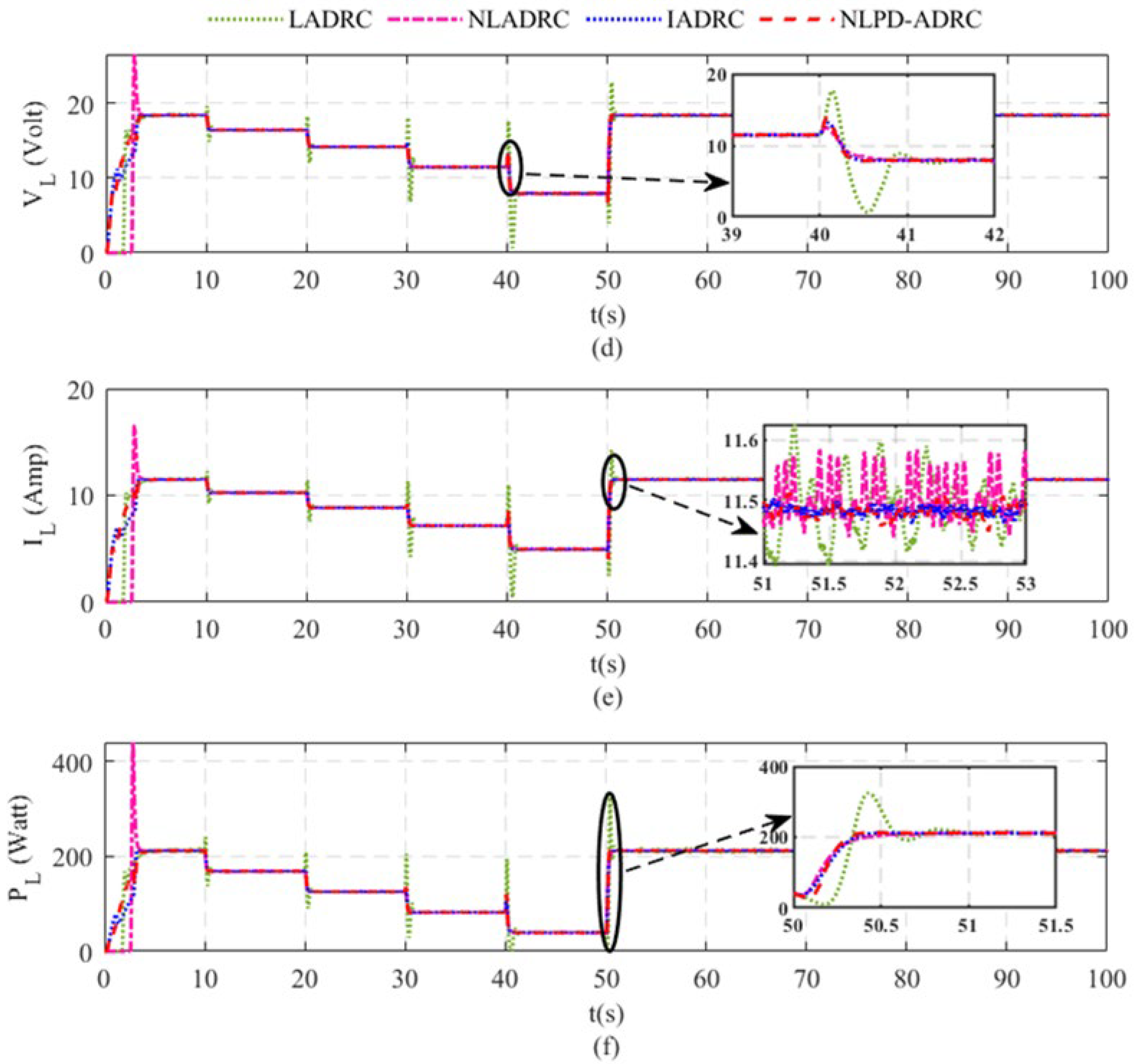
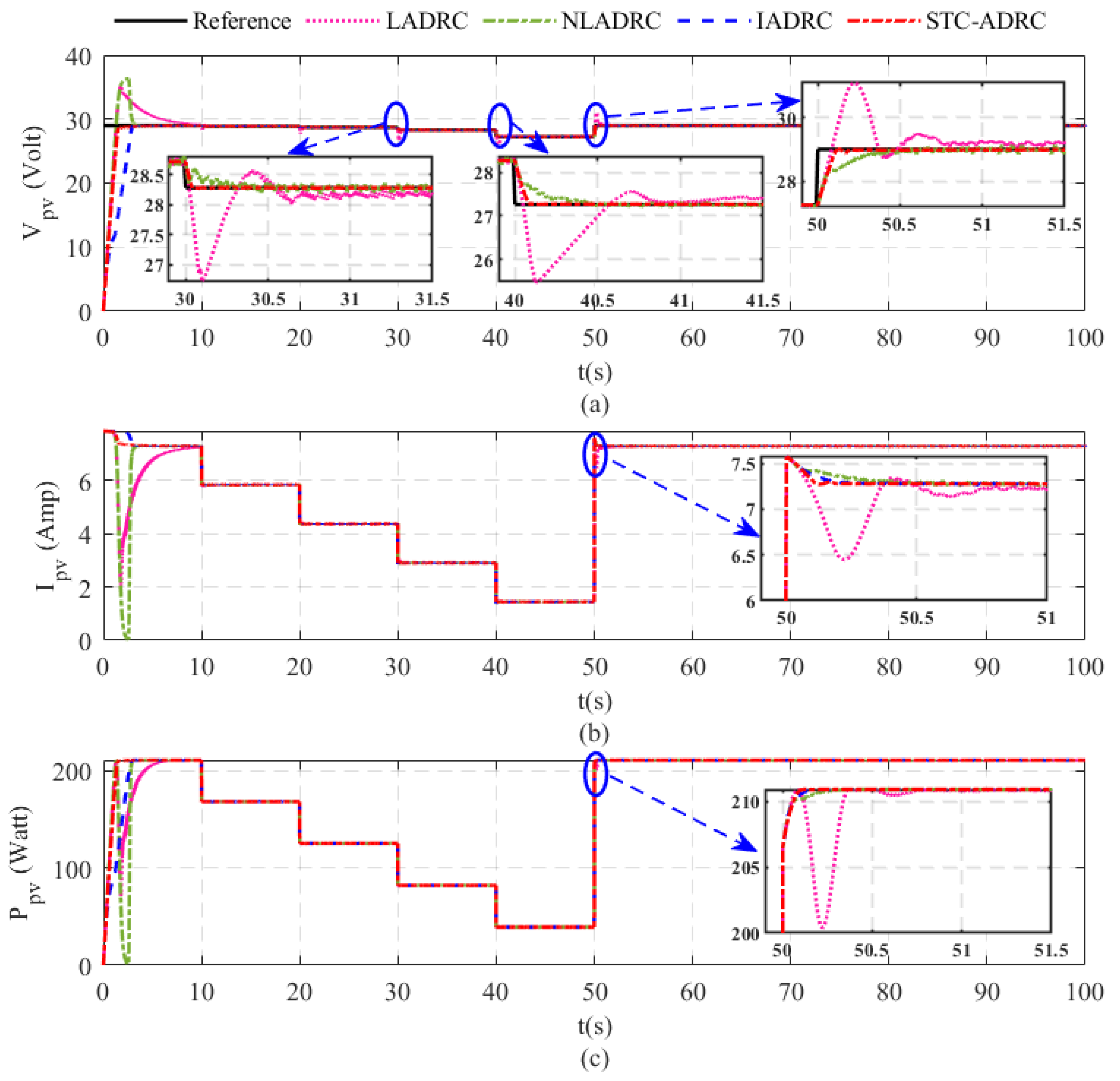
The obtained simulation results of case study one are shown in the figures below. As can be seen from Figure 5, as the irradiation decreases the output power and the voltage decreases, too. Consequently, the effect of changing the irradiation is very clear and could be considered an exogenous disturbance. Figure 5a–c shows the output response of the single solar cell in the solar panel that consists of ten PV modules connected in series, so the PV voltage of the PV module will be ten times that of the single cell, and the PV output current will be the same as in the single PV cell. It was observed that the LADRC shows an undershoot of $25.44 \mathrm{V}$ (i.e., about $6.677\%$ of the steady-state) and an overshoot of $1.27\%$ with a ripple of $0.14 \mathrm{V}$. Moreover, the classical ADRC shows a ripple of $0.05 \mathrm{V}$ and lasts for about $4 \mathrm{s}$ to reach a steady state. Moreover, the IADRC shows a reduction in the ripple and reaches the steady-state at about $1.5 \mathrm{s}$, while the proposed method shows a smooth response without a visible peak or ripple and reaches the steady-state at about $0.06 \mathrm{s}$ and was able to track the MPP for different irradiation. Similarly, from Figure 5b,c, it can be observed that the proposed method shows a better result than the other methods. Figure 5d–f shows the converter output response, and it appears that the LADRC is the one that is most affected by the rapid change in the irradiation, with an overshoot and undershoot of $51.61\%$ and $92.33\%$ of the steady-state, respectively, while the proposed method, ADRC and IADRC, shows a small peak. Moreover, the LADRC and the classical ADRC show a visible high ripple in the converter output current, while the proposed method shows a very small ripple as compared with other methods. Finally, for the converter output power, Figure 5f shows an oscillation in the response of the LADRC before reaching the steady-state; however, the proposed method shows a smooth response with robust and accurate tracking.

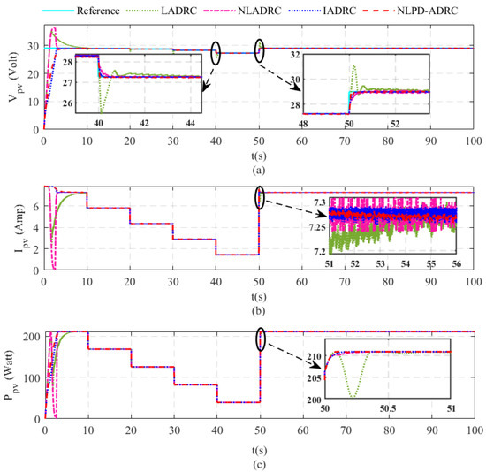
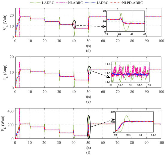
Figure 5. Comparison between the proposed method (NLPD-ADRC) and LADRC, NLADRC, and IADRC under the irradiance change. (a) PV Voltage. (b) PV Current. (c) PV Power. (d) The converter output voltage (Load Voltage). (e) The converter output current (Load Current). (f) The converter output power (Load Power).

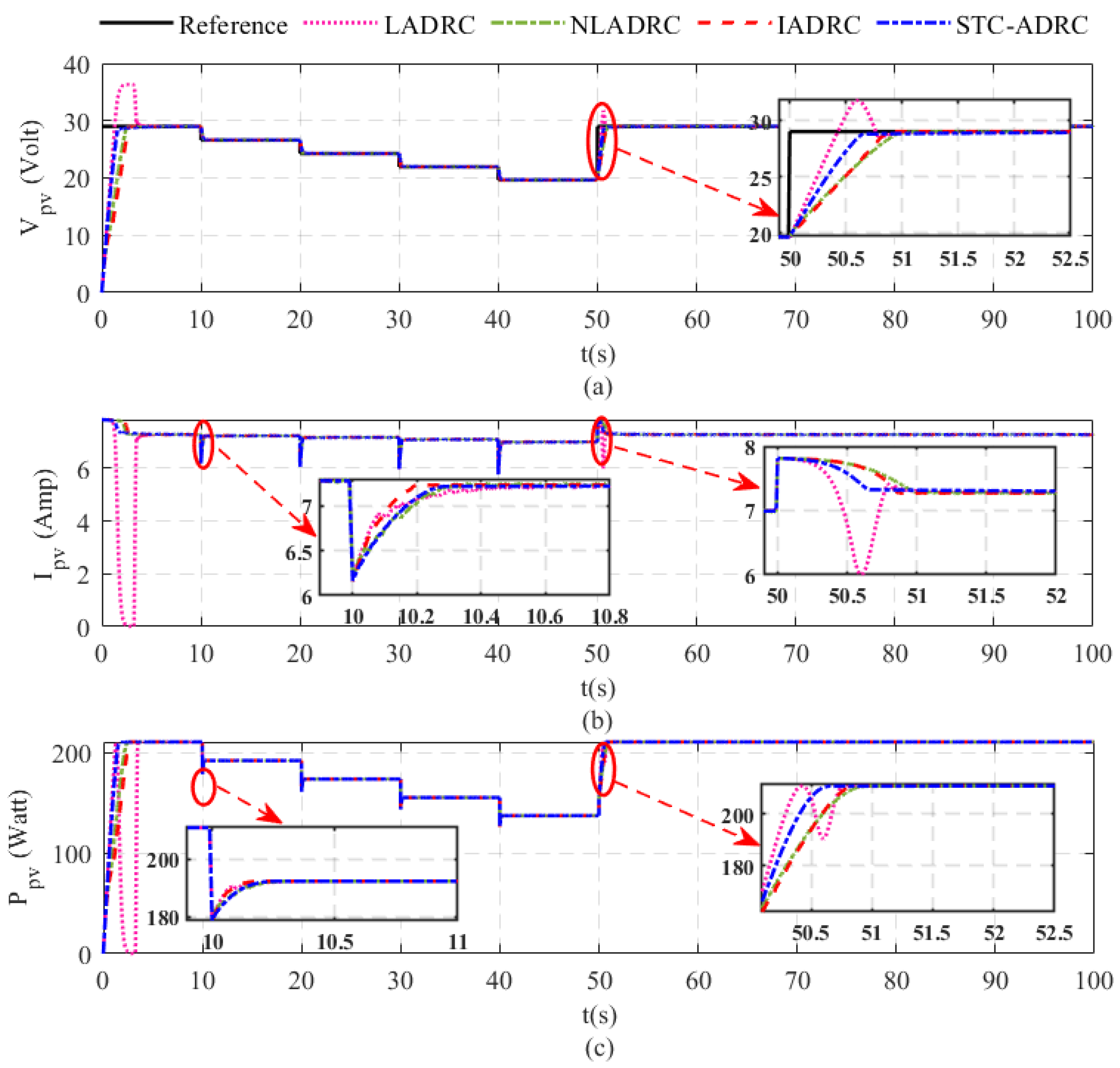
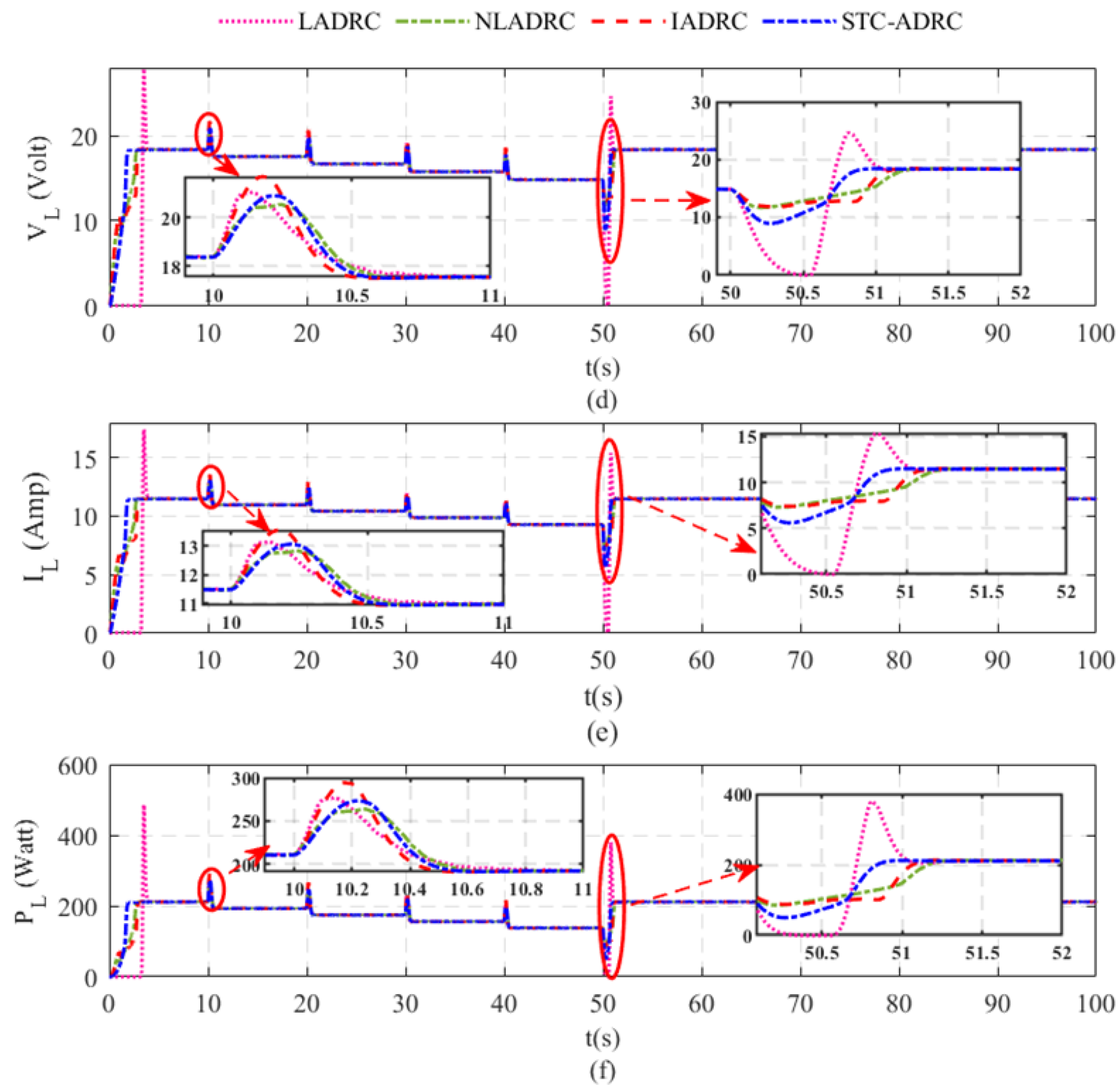
Figure 6a–c shows the output response of the PV cell. Meanwhile, Figure 6d–f represents the converter output voltage, current, and power, respectively. It clearly shows that the proposed method represents a smooth response and accurately tracks the MPP. Moreover, the obtained result shows a ripple-free and unnoticeable peak. Thus, the proposed method is more accurate with robustness against the periodic change in irradiation. It is noteworthy that the discussion of the compared methods is the same as in Figure 5, mentioned previously, except that the proposed method in Figure 6 adopted the proposed STC instead of the proposed NLPD.

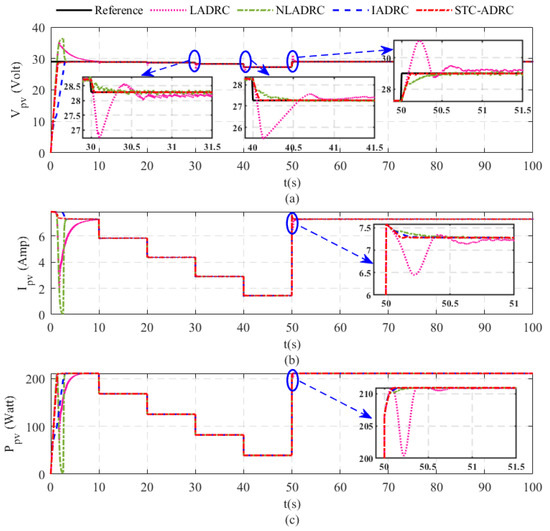
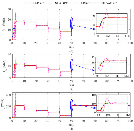
Figure 6. Comparison between the proposed method (STC-ADRC) and LADRC, NLADRC, and IADRC under irradiance changes. (a) PV Voltage. (b) PV Current. (c) PV Power. (d) The converter output voltage (Load Voltage). (e) The converter output current (Load Current). (f) The converter output power (Load Power).

ii.

Case study two. Temperature changes with constant irradiation at standard temperature conditions (STC).

In this test, a different temperature was applied with a different value at different times to observe the effect of temperature on the PV module and investigate the effectiveness of the proposed method. Figure 7a–c shows the output response of the PV module under reference and temperature changes, while Figure 7d–f shows the converter output voltage, current, and power transmitted to the load, respectively. From Figure 7, it is obvious that as the temperature increases, the power decreases, and the inverse relationship between the temperature and the power is obvious in the figure. As can be seen, the proposed method provides a smooth response with fast-tracking to the reference voltage and is also more robust, without any visible ripples or chattering. Moreover, the proposed method shows better performance, reaches the steady-state value in less $1 \mathrm{s},$ and effectively tracks the MPP. On the other hand, the LADRC shows an overshoot of $7.28 \mathrm{V},$ about $25.1\%$ of the steady-state value, the same for Figure 7b,c. The LADRC shows an undershoot with chattering in the output response. Moreover, the ADRC shows a small chattering in the output response; however, IADRC shows better results than both LADRC and ADRC and the proposed method provides excellent response and performance compared to the other methods. Moreover, as shown in Figure 7d–f, the voltage, current, and power transmitted to the load from the converter of the proposed method show a smooth response compared to the other methods. However, the IADRC also shows a good result compared to both the ADRC and LADRC, but still, the proposed method achieves an accurate and excellent performance with a minimum OPI compared to the other methods.

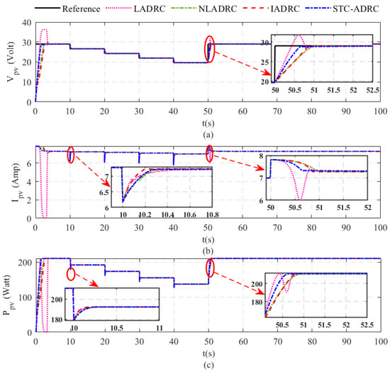
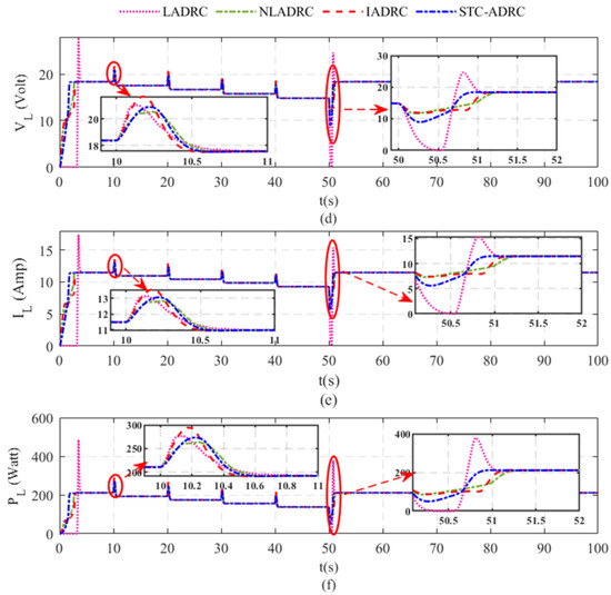
Figure 7. Comparison between the proposed method (NLPD-ADRC) and LADRC, NLADRC, and IADRC under the temperature change. (a) PV Voltage. (b) PV Current. (c) PV Power. (d) The converter output voltage (Load Voltage). (e) The converter output current (Load Current). (f) The converter output power (Load Power).

iii.

Case study three: load change with both irradiation and temperature at standard temperature conditions (STC).

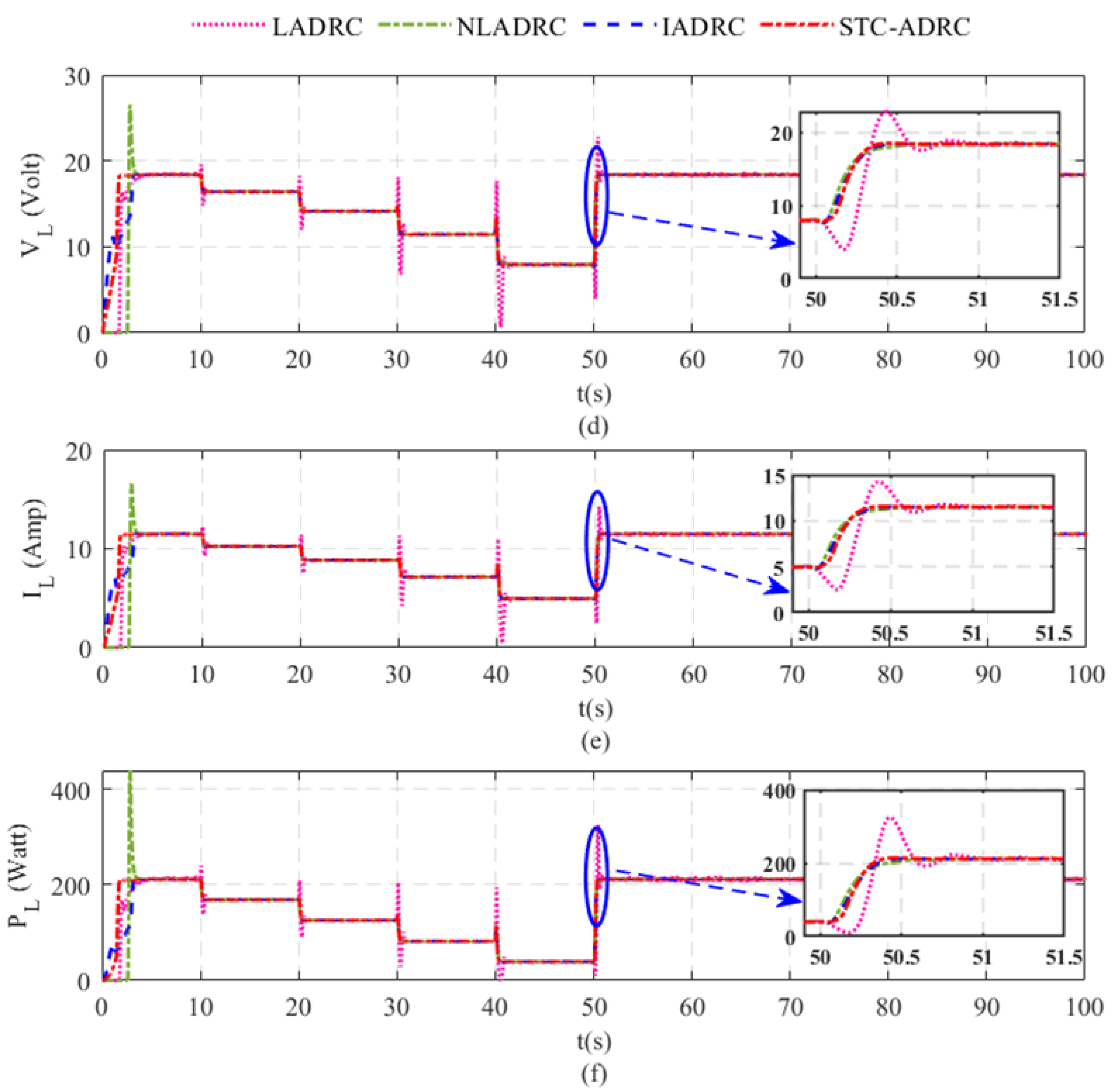
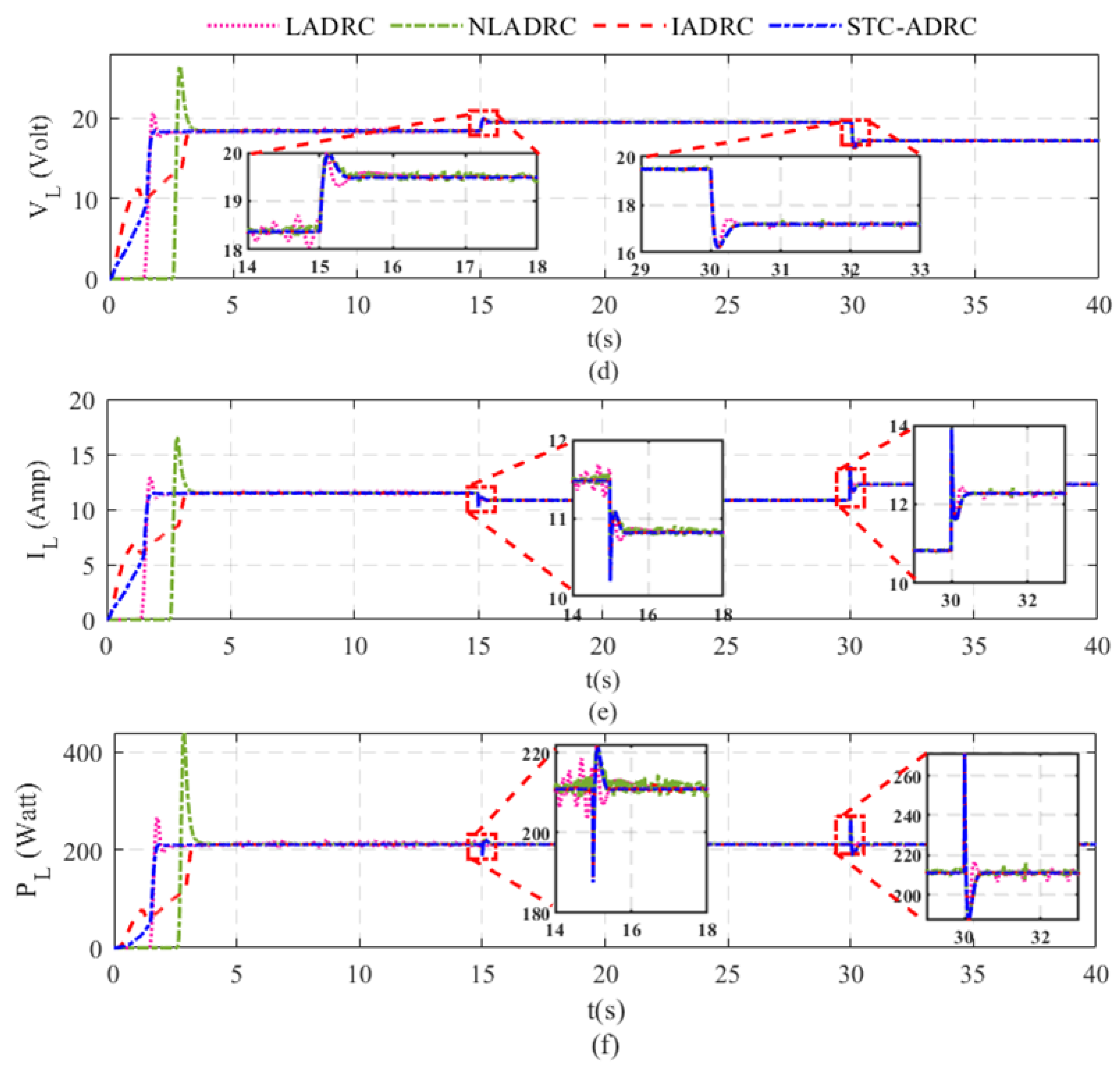
In this test, the effect of changing the load on the system is taken into consideration as an uncertainty in the load or a sudden variation in the load. The same as in the aforementioned tests, a step function of $29 u\left(t\right)$ is used as a reference. A step of $\Delta R_L\mp 20\% R_L$ is applied to observe the effect of load variation on the PV output response at $t=15 \mathrm{s}, \Delta R_L=+20\% R_L$ and $t=30 \mathrm{s},\Delta R_L=-20\% R_L$. From Figure 8a–c shown below, it appears that the proposed method is more accurate and robust with a smooth response. Moreover, the system operates at the MPP despite the load change, and this is the aim of using the proposed method, in which at any load value, the system will operate at the MPP. Moreover, the proposed method is ripple-free and reaches the steady-state at about $1.5 \mathrm{s}$ compared to the other methods. Figure 8d–f shows the converter output response. The proposed method shows a smooth response, ripple- and oscillation-free compared to the other methods; however, the IADRC also shows a good result compared to both the ADRC and LADRC. The performance index is shown in Table 10.

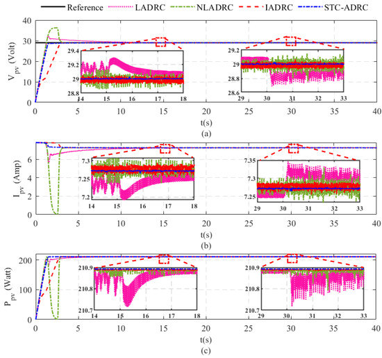
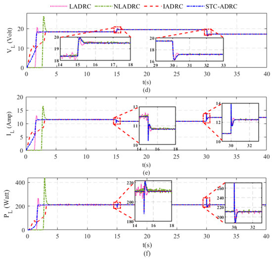
Figure 8. Comparison between the proposed method (STC-ADRC) and LADRC, NLADRC, and IADRC under load changes by $\Delta R_L=\pm 20\%$. (a) PV Voltage. (b) PV Current. (c) PV Power. (d) The converter output voltage (Load Voltage). (e) The converter output current (Load Current). (f) The converter output power (Load Power).

Table 10. The performance indices.

Performance Index	LADRC	ADRC	IADRC	NLPD-ADRC	STC-ADRC
$ITAE$	$227.645291$	$123.466037$	$113.083615$	$81.377283$	$34.246021$
$IAU$	$3124.721304$	$1738.772900$	$957.928495$	$1275.646277$	$1101.477163$
$ISU$	$1365.077613$	$112.698850$	$3.401035$	$9.959110$	$7.666228$
$OPI$	$3.742875$	$0.721694$	$0.402827$	$0.351374$	$0.199233$

Table 10 presents the performance indices. It is observed from this table that the proposed scheme shows an improvement in terms of the OPI, whereas the OPI shows an improvement of about $94.67\%$ as compared to the other schemes. Once again, the proposed method shows the best output result with minimum OPI even when applying different case studies. The proposed method proves its competence in dealing with the disturbance and uncertainties. The configuration of different ADRC schemes that used in this work are introduced in Appendix A.

7. Conclusions

In this work, two improved ADRC schemes have been proposed to design an accurate MPPT controller to operate the PV cell at the MPP in the presence of exogenous disturbances and parameter variations using super twisting sliding mode and nonlinear proportional-derivative control techniques. It can be concluded that the proposed schemes outperformed the traditional ones with a big difference in the output performance. This improvement in the performance appeared in the values of the OPI, the time-domain measures (e.g., overshoot, steady-state error), and minimum settling time, which are listed in Table 10. It is observed from this table that the proposed scheme shows an improvement in terms of the OPI, whereas the OPI shows an improvement of about $94.67\%$ as compared to the other schemes. Once again, the proposed method shows the best output result with minimum OPI even when applying different case studies. The proposed method proves its competence in dealing with the disturbance and uncertainties. Moreover, the closed-loop stability with IADRC has been analyzed using the Lyapunov stability method. The simulation results illustrated the effectiveness of the proposed schemes in tracking the MPP with a smooth, fast response and the quick attenuation of the effect of the applied disturbance and uncertainty. Finally, an extension to this work includes using different optimization algorithms in the tuning process of the controller and observer parameters and the H/W implementation of the current work using ARDUINO kits.

Appendix A.1. The Configuration of the ADRC Schemes

1.

ADRC

Figure A1. General ADRC configuration.

Figure A1. General ADRC configuration.

2.

LADRC

Figure A2. LADRC configuration.

Figure A2. LADRC configuration.

Where LSEF stands for linear state error feedback and LESO stands for linear extended state observer.

3.

IADRC, STC-ADRC, and NLPD-ADRC

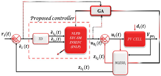
Figure A3. IADRC, STC-ADRC, and NLOD-ADR configurations.

Figure A3. IADRC, STC-ADRC, and NLOD-ADR configurations.

The ADRC schemes of IADRC, STC-ADRC, and NLPD-ADRC are the same; the difference is in the kind of the nonlinear controller used, i.e., when a super twisting sliding mode controller is used, the ADRC is called STC-ADRC, the same for the other schemes.

Appendix A.2. The Significance of the Different ADRC Schemes

The basic ADRC configuration as proposed by Han [26] takes from modern control theory’s best offering: the state observer, which embraces the power of nonlinear feedback and puts it to full use. It is a useful digital control technology developed out of an experimental platform rooted in computer simulations. The LADRC, on the other hand, inherits from proportional-integral-derivative (PID) the quality that makes it such a success: the error-driven, rather than model-based, control law. Moreover, STC-ADRC and NLPD-ADRC provide more accurate error tracking and smoother output signals than the standard ADRC and the LADRC due to the nonlinearities in the controller unit. The estimated states with the STC-ADRC and NLPD-ADRC are closer to the actual system states while the disturbance rejection is improved.

References

- Nimrod, V.; Vázquez, J. Photovoltaic System Conversion. In Power Electronics Handbook; Butterworth-Heinemann: Oxford, UK, 2018. [Google Scholar] [CrossRef]
- Baba, A.O.; Liu, G.; Chen, X. Classification and Evaluation Review of Maximum Power Point Tracking Methods. Sustain. Futures 2020, 2, 100020. [Google Scholar] [CrossRef]
- Shalaby, R.; Ammar, H.H.; Azar, A.T.; Mahmoud, M.I. Optimal Fractional-Order Fuzzy-MPPT for solar water pumping system. J. Intell. Fuzzy Syst. 2021, 40, 1175–1190. [Google Scholar] [CrossRef]
- Fekik, A.; Azar, A.T.; Denoun, H.; Kamal, N.A.; Bahgaat, N.K.; Gorripotu, T.S.; Pilla, R.; Serrano, F.E.; Mittal, S.; Rana, K.P.S.; et al. Improvement of Fuel Cell MPPT Performance with a Fuzzy Logic Controller. In Advances in Nonlinear Dynamics and Chaos (ANDC); Academic Press: Cambridge, MA, USA, 2021; pp. 161–181. [Google Scholar] [CrossRef]
- Fekik, A.; Azar, A.T.; Kamal, N.A.; Serrano, F.E.; Hamida, M.L.; Denoun, H.; Yassa, N. Maximum Power Extraction from a Photovoltaic Panel Connected to a Multi-cell Converter. In Advances in Intelligent Systems and Computing, Proceedings of the International Conference on Advanced Intelligent Systems and Informatics 2020 (AISI 2020), Cairo, Egypt, 19–21 October 2020; Hassanien, A.E., Slowik, A., Snášel, V., El-Deeb, H., Tolba, F.M., Eds.; Springer: Cham, Switzerland, 2021; Volume 1261. [Google Scholar] [CrossRef]
- Rana, K.P.S.; Kumar, V.; Sehgal, N.; George, S.; Azar, A.T. Efficient Maximum Power Point Tracking in Fuel Cell Using the Fractional-Order PID Controller. In Advances in Nonlinear Dynamics and Chaos (ANDC); Academic Press: Cambridge, MA, USA, 2021; pp. 111–132. [Google Scholar] [CrossRef]
- Azar, A.T.; Serrano, F.E.; Flores, M.A.; Kamal, N.A.; Ruiz, F.; Ibraheem, I.K.; Humaidi, A.J.; Fekik, A.; Alain, K.S.T.; Romanic, K.; et al. Fractional-Order Controller Design and Implementation for Maximum Power Point Tracking in Photovoltaic Panels. In Advances in Nonlinear Dynamics and Chaos (ANDC); Academic Press: Cambridge, MA, USA, 2021; pp. 255–277. [Google Scholar] [CrossRef]
- Kamal, N.A.; Azar, A.T.; Elbasuony, G.S.; Almustafa, K.A.; Almakhles, D. PSO-Based Adaptive Perturb and Observe MPPT Technique for Photovoltaic Systems. In Advances in Intelligent Systems and Computing, Proceedings of the International Conference on Advanced Intelligent Systems and Informatics AISI 2019, Cairo, Egypt, 26–28 October 2019; Springer: Berlin/Heidelberg, Germany, 2020; Volume 1058, pp. 125–135. [Google Scholar]
- Ammar, H.H.; Azar, A.T.; Shalaby, R.; Mahmoud, M.I. Metaheuristic Optimization of Fractional Order Incremental Conductance (FO-INC) Maximum Power Point Tracking (MPPT). Complexity 2019, 2019, 7687891. [Google Scholar] [CrossRef]
- Ko, J.S.; Huh, J.H.; Kim, J.C. Overview of Maximum Power Point Tracking Methods for PV System in Micro Grid. Electronics 2020, 9, 816. [Google Scholar] [CrossRef]
- Sharma, R.S.; Katti, P.K. Perturb & observation MPPT algorithm for solar photovoltaic system. In Proceedings of the 2017 International Conference on Circuit, Power and Computing Technologies (ICCPCT), Kollam, India, 20–21 April 2017; pp. 1–6. [Google Scholar] [CrossRef]
- Kamran, M.; Muddassar, M.; Fazal, M.R.; Asghar, M.U.; Bilal, M.; Asghar, R. Implementation of improved Perturb & Observe MPPT technique with confined search space for standalone photovoltaic system. J. King Saud Univ.-Eng. Sci. 2020, 32, 432–441. [Google Scholar] [CrossRef]
- Dhaouadi, G.; Djamel, O.; Youcef, S.; Salah, C. Implementation of Incremental Conductance Based MPPT Algorithm for Photovoltaic System. In Proceedings of the 2019 4th International Conference on Power Electronics and their Applications (ICPEA), Elazig, Turkey, 25–27 September 2019; pp. 1–5. [Google Scholar] [CrossRef]
- Shang, L.; Guo, H.; Zhu, W. An improved MPPT control strategy based on incremental conductance algorithm. Prot. Control Mod. Power Syst. 2020, 5, 14. [Google Scholar] [CrossRef]
- Narendiran, S.; Sahoo, S.K.; Das, R.; Sahoo, A.K. Fuzzy logic controller based maximum power point tracking for PV system. In Proceedings of the 2016 3rd International Conference on Electrical Energy Systems (ICEES), Chennai, India, 17–19 March 2016; pp. 29–34. [Google Scholar] [CrossRef]
- Jyothy, L.P.N.; Sindhu, M.R. An Artificial Neural Network based MPPT Algorithm for Solar PV System. In Proceedings of the 2018 4th International Conference on Electrical Energy Systems (ICEES), Chennai, India, 7–9 February 2018; pp. 375–380. [Google Scholar] [CrossRef]
- Atawi, I.E.; Kassem, A.M. Optimal Control Based on Maximum Power Point Tracking (MPPT) of an Autonomous Hybrid Photovoltaic/Storage System in Micro Grid Applications. Energies 2017, 10, 643. [Google Scholar] [CrossRef]
- Darab, C.; Turcu, A.; Stefanescu, S.; Botezan, A.; Pica, C.; Pavel, S.; Abdourraziq, S. Robust control of MPPT of a PV cell. In Proceedings of the 2017 International Conference on Electromechanical and Power Systems (SIELMEN), Iasi, Romania, 11–13 October 2017; pp. 42–46. [Google Scholar] [CrossRef]
- Irwanto, M.; Zhe, L.W.; Ismail, B.; Baharudin, N.H.; Juliangga, R.; Alam, H.; Masri, M. Photovoltaic powered DC-DC boost converter based on PID controller for battery charging system. J. Phys. Conf. Ser. 2020, 1432, 012055. [Google Scholar] [CrossRef]
- Jeba, P.; Selvakumar, A.I. FOPID based MPPT for photovoltaic system. Energy Sources Part A Recovery Util. Environ. Eff. 2018, 40, 1591–1603. [Google Scholar] [CrossRef]
- Mirza, A.F.; Mansoor, M.; Ling, Q.; Khan, M.I.; Aldossary, O.M. Advanced Variable Step Size Incremental Conductance MPPT for a Standalone PV System Utilizing a GA-Tuned PID Controller. Energies 2020, 13, 4153. [Google Scholar] [CrossRef]
- Kler, V.; Rana, K.; Kumar, V. A Nonlinear PID Controller Based Novel Maximum Power Point Tracker for PV Systems. J. Frankl. Inst. 2018, 355, 7827–7864. [Google Scholar] [CrossRef]
- Pathak, D.; Sagar, G.; Gaur, P. An Application of Intelligent Non-linear Discrete-PID Controller for MPPT of PV System. Procedia Comput. Sci. 2020, 167, 1574–1583. [Google Scholar] [CrossRef]
- Deshpande, A.S.; Patil, S.L. Robust Observer-Based Sliding Mode Control for Maximum Power Point Tracking. J. Control. Autom. Electr. Syst. 2020, 31, 1210–1220. [Google Scholar] [CrossRef]
- Pandey, S.; Deshpande, A. Maximum Power Point Tracking Using Disturbance Observer-Based Sliding Mode Control for Estimation of Solar Array Voltage. Electr. Power Compon. Syst. 2020, 48, 148–161. [Google Scholar] [CrossRef]
- Han, J. From PID to Active disturbance rejection control. Ind. Electron. 2009, 56, 900–906. [Google Scholar] [CrossRef]
- Gao, Z.; Li, S.; Zhou, X.; Ma, Y.; Zhao, J. A new maximum power point tracking method for PV system. In Proceedings of the 2017 29th Chinese Control and Decision Conference (CCDC), Chongqing, China, 28–30 May 2017; pp. 544–548. [Google Scholar] [CrossRef]
- Benrabah, A.; Khoucha, F.; Raza, A.; Xu, D. A New Robust Control for Grid Connected Photovoltaic Systems Based on Active Disturbance Rejection Control. J. Electr. Syst. 2019, 15, 81–95. [Google Scholar]
- Ramirez, E.G.; Barbosa, A.M.; Ordaz, M.A.C.; Ramirez, G.G. FPGA-based active disturbance rejection control and maximum power point tracking for a photovoltaic system. Int. Trans. Electr. Energy Syst. 2020, 30, e12398. [Google Scholar] [CrossRef]
- Zhou, X.; Liu, Q.; Ma, Y.; Xie, B. DC-Link Voltage Research of Photovoltaic Grid-Connected Inverter Using Improved Active Disturbance Rejection Control. IEEE Access 2021, 9, 9884–9894. [Google Scholar] [CrossRef]
- Hou, G.; Ke, Y.; Huang, C. A flexible constant power generation scheme for photovoltaic system by error-based active disturbance rejection control and perturb & observe. Energy 2021, 237, 121646. [Google Scholar] [CrossRef]
- Rashid, M.H. Power Electronic Handbook, 4th ed.; Elsevier: Amsterdam, The Netherlands, 2018. [Google Scholar] [CrossRef]
- Toumi, D.; Benattous, D.; Ibrahim, A.; Abdul-Ghaffar, H.I.; Obukhov, S.; Aboelsaud, R.; Labbi, Y.; Diab, A.A.Z. Optimal design and analysis of DC-DC converter with maximum power controller for stand-alone PV system. Energy Rep. 2021, 7, 4951–4960. [Google Scholar] [CrossRef]
- Baharudin, N.; Mansur, T.M.N.T.; Abdul- Hamid, F.; Ali, R.; Misrun, M.R. Topologies of DC-DC converter in solar PV applications. Indones. J. Electr. Eng. Comput. Sci. 2017, 8, 368–374. [Google Scholar] [CrossRef]
- Pandiarajan, N.; Muthu, R. Mathematical modeling of photovoltaic module with Simulink. In Proceedings of the 2011 1st International Conference on Electrical Energy Systems, Chennai, India, 3–5 January 2011; pp. 258–263. [Google Scholar] [CrossRef]
- Iftikhar, R.; Ahmad, I.; Arsalan, M.; Naz, N.; Ali, N.; Armghan, H. MPPT for Photovoltaic System Using Nonlinear Controller. Int. J. Photoenergy 2018, 2018, 6979723. [Google Scholar] [CrossRef]
- Zeb, K.; Busarello, T.D.C.; Islam, S.U.; Uddin, W.; Raghavendra, K.V.G.; Khan, M.A.; Kim, H.J. Design of Super Twisting Sliding Mode Controller for a Three-Phase Grid-connected Photovoltaic System under Normal and Abnormal Conditions. Energies 2020, 13, 3773. [Google Scholar] [CrossRef]
- Shtessel, Y.; Fridman, L.; Edwards, C.; Levant, A. Sliding Mode Control and Observation; Springer: New York, NY, USA; Heidelberg, Germany; Dordrecht, The Netherlands; London, UK, 2014; ISBN 978-0-8176-4892-3/978-0-8176-4893-0. [Google Scholar] [CrossRef]
- Gao, Z. Scaling and bandwidth-parameterization based controller tuning. In Proceedings of the 2003 American Control Conference, Denver, CO, USA, 4–6 June 2003; pp. 4989–4996. [Google Scholar] [CrossRef]
- Zheng, Q. On Active Disturbance Rejection Control; Stability Analysis and Applications in Disturbance Decoupling Control. Ph.D. Thesis, Cleveland State University, Cleveland, OH, USA, 2009. Available online: https://engagedscholarship.csuohio.edu/etdarchive/324 (accessed on 20 June 2022).
- Khalil, K.H. Nonlinear Control, Global Edition; Pearson Education: Essex, UK, 2015. [Google Scholar]
- Najm, A.A.; Ibraheem, I.K. Altitude and Attitude Stabilization of UAV Quadrotor System using Improved Active Disturbance Rejection Control. Arab. J. Sci. Eng. 2020, 45, 1985–1999. [Google Scholar] [CrossRef]
- Arsalan, M.; Iftikhar, R.; Ahmad, I.; Hasan, A.; Sabahat, K.; Javeria, A. MPPT for photovoltaic system using nonlinear backstepping controller with integral action. Sol. Energy 2018, 170, 192–200. [Google Scholar] [CrossRef]
- Abdul-Adheem, W.R.; Ibraheem, I.K. From PID to Nonlinear State Error Feedback Controller. Int. J. Adv. Comput. Sci. Appl. (IJACSA) 2017, 8, 312–322. [Google Scholar] [CrossRef]
- Abdul-Adheem, W.R.; Ibraheem, I.K. Improved Sliding Mode Nonlinear Extended State Observer based Active Disturbance Rejection Control for Uncertain Systems with Unknown Total Disturbance. Int. J. Adv. Comput. Sci. Appl. (IJACSA) 2016, 7, 80–93. [Google Scholar]
Publisher’s Note: MDPI stays neutral with regard to jurisdictional claims in published maps and institutional affiliations. |
© 2022 by the authors. Licensee MDPI, Basel, Switzerland. This article is an open access article distributed under the terms and conditions of the Creative Commons Attribution (CC BY) license (https://creativecommons.org/licenses/by/4.0/).